Classifying Classic Ciphers using Machine Learning

San Jose State University

SJSU ScholarWorks

Master's Projects Master's Theses and Graduate Research

Spring 5-20-2019

Classifying Classic Ciphers using Machine

Learning

Nivedhitha Ramarathnam Krishna

Follow this and additional works at:https://scholarworks.sjsu.edu/etd_projects

Part of theArtificial Intelligence and Robotics Commons, and theInformation Security

Commons

This Master's Project is brought to you for free and open access by the Master's Theses and Graduate Research at SJSU ScholarWorks. It has been accepted for inclusion in Master's Projects by an authorized administrator of SJSU ScholarWorks. For more information, please contact

Recommended Citation

Krishna, Nivedhitha Ramarathnam, "Classifying Classic Ciphers using Machine Learning" (2019).Master's Projects. 699. DOI: https://doi.org/10.31979/etd.xkgs-5gy6

Classifying Classic Ciphers using Machine Learning

A Project Presented to

The Faculty of the Department of Computer Science San José State University

In Partial Fulfillment

of the Requirements for the Degree Master of Science

by

Nivedhitha Ramarathnam Krishna May 2019

© 2019

Nivedhitha Ramarathnam Krishna ALL RIGHTS RESERVED

The Designated Project Committee Approves the Project Titled Classifying Classic Ciphers using Machine Learning

by

Nivedhitha Ramarathnam Krishna

APPROVED FOR THE DEPARTMENT OF COMPUTER SCIENCE SAN JOSÉ STATE UNIVERSITY

May 2019

Dr. Mark Stamp Department of Computer Science Dr. Thomas Austin Department of Computer Science Professor Fabio Di Troia Department of Computer Science

ABSTRACT

Classifying Classic Ciphers using Machine Learning by Nivedhitha Ramarathnam Krishna

We consider the problem of identifying the classic cipher that was used to generate a given ciphertext message. We assume that the plaintext is English and we restrict our attention to ciphertext consisting only of alphabetic characters. Among the classic ciphers considered are the simple substitution, Vigenère cipher, playfair cipher, and column transposition cipher. The problem of classification is approached in two ways. The first method uses support vector machines (SVM) trained directly on ciphertext to classify the ciphers. In the second approach, we train hidden Markov models (HMM) on each ciphertext message, then use these trained HMMs as features for classifiers. Under this second approach, we compare two classification strategies, namely, convolutional neural networks (CNN) and SVMs. For the CNN classifier, we convert the trained HMMs into images. Extensive experimental results are provided for each of these classification techniques.

ACKNOWLEDGMENTS

I would like to extend my sincere gratitude to my advisor Dr. Mark Stamp for encouraging me to experiment with new topics and for helping me with his expertise from the very beginning. I would like to thank Professor Fabio Di Troia for his constant guidance. His insightful ideas and suggestions, helped me extend my research from different perspectives. I would like to thank Dr. Thomas Austin for his continuous support and encouragement throughout my research.

TABLE OF CONTENTS

CHAPTER

1 Introduction . . . 1

2 Background . . . 3

2.1 Classic ciphers . . . 3

2.1.1 Simple substitution cipher . . . 3

2.1.2 Vigenère cipher . . . 3

2.1.3 Column transposition cipher . . . 4

2.1.4 Playfair cipher . . . 5

2.2 Previous work . . . 6

2.3 Overview of proposed approach . . . 7

2.4 Machine learning algorithms . . . 8

2.4.1 Hidden Markov model . . . 8

2.4.2 Convolutional neural network . . . 10

2.4.3 Support vector machine . . . 11

3 Implementation . . . 15

3.1 Training SVMs on ciphertexts (technique 1) . . . 15

3.1.1 Dataset preparation for SVM . . . 15

3.2 Training HMMs on ciphertexts . . . 16

3.2.1 Simple substitution cryptanalysis . . . 16

3.2.2 Vigenère cryptanalysis . . . 17

3.2.4 Playfair cryptanalysis . . . 19

3.3 Training CNNs on pretrained HMMs (technique 2) . . . 19

3.3.1 Dataset preparation for CNN . . . 19

3.4 Training SVMs on pretrained HMMs (technique 3) . . . 21

3.4.1 Dataset preparation for SVM . . . 21

4 Experiments and Results . . . 22

4.1 Results for technique 1 . . . 22

4.2 Results for technique 2 . . . 22

4.3 Results for technique 3 . . . 26

5 Conclusion . . . 33

LIST OF REFERENCES . . . 35

APPENDIX Appendix A . . . 38

A.1 Results for technique 1 . . . 38

A.2 Results for technique 3 . . . 38

A.3 Results for technique 2 . . . 39

A.3.1 ROC plots for CNN having two convolution layers . . . . 39

A.3.2 Confusion matrix plots for CNN having two convolution layers . . . 41

A.3.3 ROC plots for CNN having three convolution layers . . . 42

A.3.4 Confusion matrix plots for CNN having three convolution layers . . . 43

LIST OF TABLES

1 Example of simple substitution cipher key . . . 3

2 Example of column transposition cipher key: 21354 . . . 4

3 Encryption using key: 21354 . . . 5

4 Example of playfair cipher key: ZODIAC . . . 5

5 HMM parameters notation . . . 9

6 Feature vector mapping . . . 15

7 Class labels for SVM . . . 16

8 Sample dataset used for training SVM using ciphertext . . . 16

9 Converged 𝐵 matrix of HMM trained on simple substitution cipher for𝑁 = 26 . . . 17

10 Converged 𝐵 matrix of HMM trained on Vigenère cipher for 𝑁 = 5 . . . 18

11 Converged 𝐵 matrix of HMM trained on column transposition cipher for𝑁 = 5 . . . 18

12 Converged 𝐵 matrix of HMM trained on column transposition cipher for𝑁 = 2 . . . 18

13 Converged𝐵 matrix of HMM trained on playfair cipher for 𝑁 = 5 19 14 Dataset size . . . 23

15 HMM parameters . . . 23

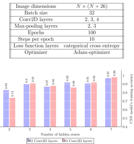
16 CNN parameters . . . 25

LIST OF FIGURES

1 Hidden Markov model [1] . . . 9

2 Convolution using filter [2] . . . 10

3 Pooling function [2] . . . 11

4 Overview of CNN architecture [2] . . . 11

5 SVM hyperplane separating data points [3] . . . 12

6 Kernel trick by projecting data to higher dimension [3] . . . 12

7 Types of kernels on Iris dataset [4] . . . 13

8 HMM 𝐴 and 𝐵 matrices converted to image for simple substitution cipher for 𝑁 = 2 . . . 20

9 HMM 𝐴 and 𝐵 matrices converted to image for Vigenère cipher for 𝑁 = 5 . . . 20

10 System implementation for technique 2 . . . 20

11 System implementation for technique 3 . . . 21

12 SVM macro-average AUC value over different lengths of ciphertexts . . . 23

13 ROC plots for SVM trained on different lengths of ciphertext . 24 14 CNN model training accuracy for 2 and 3 Con2D layers . . . 25

15 Confusion matrix plots for CNN having two Conv2D layers for 𝑁 as 2,4,5,7 . . . 26

16 Converged HMM images for Vigenère and playfair ciphers for 𝑁 = 5 and 𝑁 = 7 . . . 27

17 Confusion matrix for𝑁 = 2 . . . 27

19 Confusion matrix for𝑁 = 5 . . . 28

20 ROC for 𝑁 = 5 . . . 29

21 Confusion matrix grid for SVM trained on 1000 HMMs for each of the four cipher classes . . . 30 22 Confusion matrix grid for SVM trained on 200 HMMs for each

of the four cipher classes . . . 31 A.23 ROC plots for SVM trained on different lengths of ciphertext . 38 A.24 ROC plots for SVM trained on 200 HMMs for each of the four

cipher classes . . . 39 A.25 ROC plots for CNN having two Conv2D layers . . . 40 A.26 Confusion matrix plots for CNN having two Conv2D layers . . 41 A.27 ROC plots for CNN having three Conv2D layers . . . 42 A.28 Confusion matrix plots for CNN having three Conv2D layers . . 43 A.29 Vigenère cipher key table . . . 44

CHAPTER 1 Introduction

Cryptography includes two main tasks, namely, encryption and decryption. Encryption is the process of converting an easily readable plaintext to disguised ciphertext which is performed by the sender of the message. Decryption is the process of bringing back the plaintext or original message from the ciphertext which is performed on the receiver's end. Decryption can be easily performed by the receiver provided he/she is given the key [5]. On the other hand, deciphering the message without the key is called cryptanalysis. Cryptanalysis performs steps to analyze the weakness of ciphers in order to defeat them, which is in general a time-consuming process. Nonetheless, statistics and machine learning models can be used as tools to efficiently perform these tasks and help achieve the goal of automation, which is particularly useful in this field. The right machine learning model can be built to learn the statistics of any given language [1]. Using this trained or learned model, techniques can be analyzed to attack an encrypted text. An example of this application could be experimenting various types of classifiers to identify the classic encryption algorithm used.

This research limits the focus on applying machine learning techniques to perform cryptanalysis on classic ciphers that are generally of historical interest. These experiments provide useful insight about the hidden statistics of a given cipher and types of attacks possible, hence, helping in efficient design of an encryption system.

The aim of this research is to identify the classic cipher used to generate the ciphertext message. Two methods are considered to approach this problem. The first method lets the data speak for itself and hence, considers stand-alone ciphertexts as training data. To implement this method, ciphertexts are converted to

feature vectors and support vector machines (SVMs) are trained to fit these feature vectors. Henceforth, in this research, this technique is referred as ‘‘technique 1’’. On the other hand, the second method aims to approach this problem by capturing hidden statistics behind the ciphertext message. In order to implement this, several hidden Markov models (HMMs) are trained on four classic ciphertexts. To maintain structural dependencies of these properties, two strategies are considered. Firstly, the trained HMMs are converted to images which are finally classified using convolutional neural networks (CNNs). Henceforth, in this research, this technique is referred as ‘‘technique 2’’. Secondly, the trained HMMs are converted to one-dimensional vectors which are finally classified using SVMs. Henceforth, in this research, this technique is referred as ‘‘technique 3’’.

The report is structured as follows: Chapter 2 gives a background on classic ciphers, machine learning models used for this research and discusses about previous applications of machine learning in cryptanalysis. Chapter 3 describes in detail about this research's implementation. Chapter 4 gives a detailed explanation on the experiments and results of this research for classifying four types of cipher. Chapter 5 focuses on reviewing the goal of combining two or more machine learning techniques for effective cryptanalysis, compares it with a single-step approach and finally, discusses future scope of this research.

CHAPTER 2 Background 2.1 Classic ciphers

The history of ciphers dates back to around 1500 B.C. when clay tablets were used to hide secret recipes of craftsman for valuable goods in Mesopotamia [6]. A cipher is a way of obfuscating the actual message for protecting important information. The process of converting plain and readable text to ciphertext is called encryption. This section discusses the classic ciphers used in this research. 2.1.1 Simple substitution cipher

Simple substitution ciphers use a fixed one-to-one mapping of the letters in plaintext and ciphertext [7]. Each character of the message is mapped to a different character and this complete map constitutes the key. Ciphertext is formed by substituting every occurrence of the character in plaintext with the mapped character of the key. An example of key mapping is shown in Table 1.

Table 1: Example of simple substitution cipher key

plaintext A B C D E F G H I J K L M N O P Q R S T U V W X Y Z ciphertext F G H I J K L M N O P Q R S T U V W X Y Z A B C D E

2.1.2 Vigenère cipher

Vigenère cipher is a polyalphabetic cipher unlike simple substitution which is monoalphabetic. In a polyalphabetic cipher the mapping between plaintext and ciphertext changes, that is, more than one cipher character is used for substituting a single plaintext character. Hence, there is a one-to-many relationship between each letter and its substitutes [8].

Vigenère cipher applies a repeated series of simple substitutions on the plaintext, based on the length of the key. For example, if the length of key is 𝑚, then groups

of 𝑚 letters of plaintext are shifted by the corresponding letter of the key [5]. Let

us consider a key as

𝐾 = (𝑘1, 𝑘2, . . . , 𝑘𝑚)

then encryption occurs by

𝑒𝑘(𝑥1, 𝑥2, . . . , 𝑥𝑚) = (𝑥1+𝑘1, 𝑥2+𝑘2, . . . , 𝑥3+𝑘𝑚) mod 26

and decryption occurs by

𝑑𝑘(𝑦1, 𝑦2, . . . , 𝑦𝑚) = (𝑦1 −𝑘1, 𝑦2−𝑘2, . . . , 𝑦3−𝑘𝑚) mod 26

This cipher can also be interpreted as set of 26 Caesar's ciphers. Figure A.29 shows the 26 shifts, each row representing one cyclic shift of plaintext. Hence, according to the above formula, the character that would substitute the first plaintext letter can be found in the intersection of plaintext letter and the first character of the key [9].

2.1.3 Column transposition cipher

As the name suggests, this cipher involves permutation of the plaintext letters which are first written into a grid. Depending upon the key, the units of plaintext are rearranged in a different way [5].

Table 2: Example of column transposition cipher key: 21354

2 1 3 5 4 M E E T M E T O M O R R O W T H I S I S T H E E Z

As seen in Table 2, the columns are read out in the order of the key. The corresponding ciphertext and plaintext are shown in Table 3.

Table 3: Encryption using key: 21354

plaintext MEETMETOMORROWTHISISTHEEZ

ciphertext ETRIHMERHTEOOSEMOTSZTMWIE

2.1.4 Playfair cipher

This cipher has a fixed5×5matrix as a key table, which has all the letters of

English alphabet [10]. In order to accommodate all the 26 letters, the key table places I and J in the same cell. For each key, a 5×5matrix is generated similar to

the one shown in Table 4.

Table 4: Example of playfair cipher key: ZODIAC

Z O D I A

C B E F G

H K L M N

P Q R S T

U V W X Y

Generally, encryption and decryption occur in pairs of plaintext message (called digrams). Using the key in Table 4, and using the following the set of rules [10], encryption and decryption is applied. Firstly, the message is divided into digrams with the condition that no two letters in the pair should be identical. If identical letters are found, then a stopgap letter is inserted between them. Secondly, there are three cases possible:

• Both digram letters are in same row: The corresponding ciphertext digram are one position to the right of the plaintext letters. If any plaintext letter is the last element in any row, the corresponding ciphertext letter is the first element of the same row. Example: ciphertext of IA in Table 4 is AZ. • Both digram letters are in same column: The corresponding ciphertext digram

are one position below the plaintext letters. If any plaintext letter is the last element in any column, the corresponding ciphertext letter is the first element of the same column. Example: ciphertext of ZU in Table 4 is CZ. • Both digram letters are in opposite column of rectangle: The first character

in the ciphertext would be the character in the same row as first character of plaintext digram and last column (same column as second character of plaintext digram) and vice versa. Example: ciphertext of HD in Table 4 is LZ

2.2 Previous work

As seen earlier, the task of a cryptanalyst would be breaking the cryptosystem without having the secret key. In order to do this, the decryption function must be identified. Furthermore, in most of the attacks, the cryptanalyst would try to interpret a large number of matching ciphertexts and plaintexts. This problem could be compared to a classification or detection problem, where the goal is to find an unknown function with known inputs, outputs and classes [11]. This section discusses previous work on applications of machine learning models in the field of cryptanalysis.

Commonly used classification techniques for identifying the encryption al-gorithm include classifying the ciphertext themselves. The paper [12] discusses about capability of HMMs being able to classify between block and stream ciphers. The paper [13] compares the results from HMMs [12] to Fisher's discriminant analysis (FDA). The papers [12] and [13] collect the data in form of ciphertext's bit information, and so, ciphertext themselves are used as the training data. One similar research [14], uses neural networks to classify three classic substitution ciphertexts along with certain features. Intuitively, dealing with direct ciphertext

should not lead to much useful information. Furthermore, extracting the informa-tion from ciphertext using techniques such as 𝑛-grams might not be of advantage

here as the ciphertext does not necessarily follow natural language processing (NLP) rules [15]. In this research, technique 1 implements training classifiers on

stand-alone ciphertexts to compare the results with other strategies.

Combining two or machine learning models is discussed by a previous research, where malware files are classified by considering them as images, thus converting it to a image classification problem using CNNs [16]. Another previous research to detect metamorphic malware combines scores from different techniques, namely, HMMs, Simple Substitution Distance (SSD) and Opcode Graph Similarity (OGS) and uses a SVM to classify these scores [17]. The paper [18] considers features of classic ciphers to train neural networks. In this research, technique 2 combines multiple machine learning models to capture any hidden patterns in the input ciphertexts.

HMMs are one of the few techniques proven to have significant results in attacking classic ciphers [19]. HMMs help in capturing hidden meanings as well as probability distributions of various ciphertext letters in form of state transition matrix and emission probability matrix [19]. However, the downside of using these matrices is the fact that the hidden states might correspond to different meanings, that is generally random.

2.3 Overview of proposed approach

This section gives an overview of the machine learning models used in this research for classifying classic ciphers. This research implements a novel solution to retain the structural information of HMM matrices. This is done by converting the converged HMM matrices to images and high dimensional feature vectors.

The HMM images are classified using CNNs and the HMM vectors are classified using SVMs. This research focuses on training various HMMs on classic ciphers, mainly simple substitution, Vigenère, column transposition and playfair cipher. The encryption algorithm classification problem is transformed as an image or vector classification problem.

2.4 Machine learning algorithms

This section gives an overview of the machine learning models used in this research.

2.4.1 Hidden Markov model

Hidden Markov models (HMMs) are adaptive systems that have been exten-sively used in modeling sequences such as timeseries, DNA sequences and modeling speech recognition. HMMs, while applied in the field of cryptanalysis, have proven to give promising results [19].

Given a discrete state machine, Markov process [1] (a random process in which the future state is independent of the past state, given the present state) can identify hidden states or meanings given the observations or data. Hence, in HMM, the system's hidden states or behavior is assumed to follow the Markov process. The model captures the probabilistic nature of the sequence or models the probabilistic distributions of the observed data and their relationship with the hidden states.

Following the notation of HMM parameters in Table 5, the three main com-ponents of an HMM include the 𝐴, 𝐵 and the 𝜋 matrix. The dimensions of the

matrices depend on𝑁 (the number of hidden states) and𝑀 (the number of unique

symbols in observation). The 𝜋 matrix is a 1×𝑁 matrix where each value

cor-responds to the probability for that particular hidden state to appear first. The

𝑂0 𝑂1 𝑂2 · · · 𝑂𝑇−1

𝑋0 𝑋1 𝑋2 · · · 𝑋𝑇−1

𝐴 𝐴 𝐴 𝐴

𝐵 𝐵 𝐵 𝐵

Figure 1: Hidden Markov model [1] Table 5: HMM parameters notation Symbol Notation

𝑂 Observation sequence

𝑁 Number of hidden states

𝑀 Number of distinct symbols in 𝑂

𝑇 Length of 𝑂

𝑋 Set of hidden states in the Markov process 𝐴 State transition matrix

𝐵 Observation emission probability matrix 𝜋 Initial state probability matrix

transitioning from one hidden state to the other. The 𝐵 matrix is a𝑁×𝑀 matrix

where each value corresponds to the probability of observing that data element from that hidden state. All the matrices are row stochastic. Using these parameters an HMM can be defined as 𝜆(𝐴, 𝐵, 𝜋).

The three classic problems that are addressed using HMMs are estimating the probability of an observation sequence given the model or scoring the observation sequence against the model, finding the best hidden state sequence given observation sequence and model, and training the HMM to learn the observations [1]. The problem 3 which is training the HMM is done using Baum-Welch re-estimation

algorithm [1]. This iterative hill-climb process randomly initializes the 𝐴,𝐵 and𝜋

matrices initially and then computes new matrices using Expectation Maximization (EM) algorithm. This re-estimation process helps converge to a local maximum in the parameter space, where the parameters are the elements of the matrices that define the HMM [20].

2.4.2 Convolutional neural network

Formally, convolution is defined as an integral that calculates amount of overlap of one function as it is shifted over another function. Convolution can be also defined as a process of blending two functions [21]. Convolutional neural networks (CNNs) is a class of deep learning technique that applies layers of convolution on the input dataset with a filter dataset, that is generally learnt through the training process. Design of CNNs are inspired by the connectivity patterns of neurons of the visual cortex of the brain [22]. This takes the structural and hierarchical patterns of the observations into account and, hence, CNNs were mainly developed for computer vision [23].

Figure 2 shows a convolution function applied on input and filter function [2]. In general, the architecture followed in designing a CNN [15], stacks convolution

Figure 2: Convolution using filter [2]

layers, max-pooling layers, and fully connected layers. Two dimensional convolving filters are used sequentially in the neural network's hidden layers. These filters serve

the purpose of capturing features of the images [2]. Max-pooling function helps retain only the relevant features of the image. Figure 3 shows pooling function [2]. The fully-connected layer applies activation function and classifies the input based on this information. Figure 4 shows the complete CNN architecture [2].

Figure 3: Pooling function [2]

Figure 4: Overview of CNN architecture [2] 2.4.3 Support vector machine

Support vector machines (SVMs) are a class of supervised machine learning algorithms that can be used for both regression and classification [24]. Firstly, the algorithm represents the input data samples as points in space and these points are mapped according to the class label included in the input data. Secondly, the algorithm tries to separate these labels by finding an optimal hyperplane, in the sense of maximizing the ‘‘margin,’’ that is, the separation between classes. Test sample data that are represented onto this space, are classified depending upon which side of the hyperplane they are mapped to. The best suited hyperplane

would be the one that has maximum distance from the nearest point on either side of it. Figure 5 below shows an example of the hyperplane [25].

Figure 5: SVM hyperplane separating data points [3]

SVMs can also handle non-linear classification effectively using kernel trick [3]. This technique projects inputs to high-dimensional feature spaces as shown in Figure 6. The type of kernel to choose depends upon the type of data and problem to be solved. For non-linear classification, radial basis function (RBF) kernel is the default kernel. Figure 7 shows different types of kernels on a given dataset [4].

Figure 6: Kernel trick by projecting data to higher dimension [3]

The formula below shows loss function calculation [25]. A regularization pa-rameter can also be added to this cost function to balance the margin maximization

Figure 7: Types of kernels on Iris dataset [4] and loss. Cost function is calculated as

𝑐(𝑥, 𝑦, 𝑓(𝑥)) = ⎧ ⎪ ⎪ ⎨ ⎪ ⎪ ⎩ 0 if 𝑦𝑓(𝑥)≥1 1−𝑦𝑓(𝑥) otherwise

After regularization parameter is added, the loss function becomes

min 𝑤 𝜆||𝑤|| 2₊ 𝑛 ∑︁ 𝑖=1 (1−𝑦𝑖 < 𝑥𝑖, 𝑤 >)

Taking partial derivative of the loss function with respect to the weights gives gradients [25]. These gradients can help updating the weights. SVM partial derivative is obtained by first computing

𝜕𝜆||𝑤||2 𝜕𝑤𝑘 = 2𝜆𝑤𝑘 then 𝜕(1−𝑦𝑖(𝑥𝑖, 𝑤)) 𝜕𝑤𝑘 = ⎧ ⎪ ⎪ ⎨ ⎪ ⎪ 0 if (𝑦𝑖(𝑥𝑖, 𝑤))≥1 −𝑦 𝑥𝑖𝑘 otherwise

When the classification of the model is correct, the only update needed for the gradient is with the regularization parameter [25]. This gradient update is given by

𝑤=𝑤−𝛼(2𝜆𝑤)

On the other hand, when the classification of the model is incorrect, the update needed for the gradient includes loss and the regularization parameter [25]. In this case, the gradient update is computed as

CHAPTER 3 Implementation

3.1 Training SVMs on ciphertexts (technique 1)

For training the SVMs stand-alone ciphertexts are considered. Input to SVM must be fed in form of vectors along with their corresponding class labels. After these input feature vectors are projected into a feature space, the hyperplane helps in performing the classification as mentioned in Chapter 2. SVM is implemented using

sklearn library. StratifiedKFold [26] cross-validation is used, where number of

folds is 10. OneVsRestClassifier[27] library is used to calculate confusion matrix

and receiver operation characteristic curve (ROC). 3.1.1 Dataset preparation for SVM

Firstly, for each of the four classes of cipher, 1000 ciphertexts are created. This is implemented by encrypting a common plaintext using 1000 randomly generated keys for each cipher algorithm. The length of the ciphertext chosen for this experiment ranges between 10 and 10000. Secondly, the ciphertext consisting of 26 English alphabetic characters are simply converted to mappings of numbers between 0-25 as shown in Table 6. These mapped string of numbers are given as feature vectors along with the class labels, where each class label is mapped to each cipher as shown in Table 7.

Table 6: Feature vector mapping

characters A B C D E F G H I J K L M N O P Q R S T U V W X Y Z mapped numbers 0 1 2 3 4 5 6 7 8 9 10 11 12 13 14 15 16 17 18 19 20 21 22 23 24 25

For this research, experiments using different lengths of ciphertext are con-ducted. Table 8 shows a snapshot of feature vectors to train the SVM.

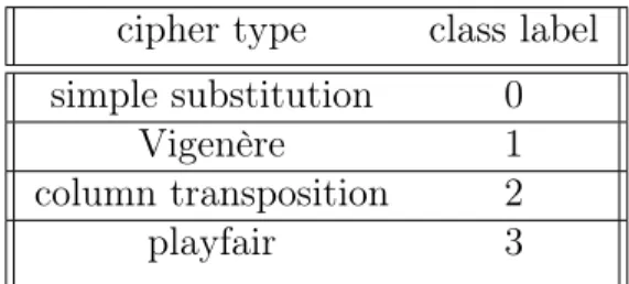
Table 7: Class labels for SVM cipher type class label simple substitution 0

Vigenère 1

column transposition 2

playfair 3

Table 8: Sample dataset used for training SVM using ciphertext

Feature vector Label

19, 7, 4, 5, 24, 11, 19, 14, 13, 2 0 19, 7, 4, 5, 22, 11, 19, 14, 13, 2 0 3, 0, 10, 7, 24, 21, 12, 20, 15, 6 1 20, 3, 2, 18, 6, 12, 15, 12, 0, 14 1 5, 13, 19, 13, 24, 5, 24, 21, 6, 13 2 19, 11, 14, 6, 9, 0, 8, 13 18, 19 2 21, 6, 5, 0, 2, 7, 21, 13, 16, 25 3 18, 15, 5, 1, 11, 1, 14, 16, 8, 5 3 3.2 Training HMMs on ciphertexts

HMMs are well-known to capture probabilistic dependencies between hidden and observed states [1]. This property gives HMMs a significantly greater advantage over other machine learning techniques to capture information between observed ciphertext and hidden plaintext [1]. Thus, providing an advantage in cryptanalysis tasks. This section gives a detailed explanation about how to apply the results captured by HMMs when they are trained on four different classic ciphertexts using different parameters.

3.2.1 Simple substitution cryptanalysis

Previous research on various attacks on simple substitution cipher has discussed advantages and disadvantages of Jakobsen's algorithm and HMM with random restarts [19]. For 𝑁 = 26, each hidden state value in 𝐵 matrix corresponds to

each character in the observation sequence, which is the ciphertext. The maximum probability value in each row shows the corresponding shift and would give us the key, which in this case is 3. Table 9 shows a converged 𝐵 matrix for 26 hidden

states.

Table 9: Converged 𝐵 matrix of HMM trained on simple substitution cipher for

𝑁 = 26 A B C D E F G H I J K L M N O P Q R S T U V W X Y Z A 0.00 0.00 0.00 0.95 0.00 0.00 0.00 0.05 0.00 0.00 0.00 0.00 0.00 0.00 0.00 0.00 0.00 0.00 0.00 0.00 0.00 0.00 0.00 0.00 0.00 0.00 B 0.00 0.00 0.00 0.00 0.55 0.00 0.00 0.00 0.01 0.20 0.00 0.00 0.09 0.00 0.00 0.00 0.00 0.00 0.16 0.00 0.00 0.00 0.00 0.00 0.00 0.00 C 0.00 0.00 0.00 0.00 0.00 0.99 0.00 0.00 0.00 0.01 0.00 0.00 0.00 0.00 0.00 0.00 0.00 0.00 0.00 0.00 0.00 0.00 0.00 0.00 0.00 0.00 D 0.00 0.00 0.00 0.00 0.00 0.00 0.75 0.00 0.00 0.20 0.00 0.00 0.00 0.01 0.04 0.00 0.00 0.00 0.00 0.00 0.00 0.00 0.00 0.00 0.00 0.00 E 0.00 0.00 0.00 0.00 0.00 0.00 0.00 1.00 0.00 0.00 0.00 0.00 0.00 0.00 0.00 0.00 0.00 0.00 0.00 0.00 0.00 0.00 0.00 0.00 0.00 0.00 F 0.00 0.00 0.00 0.00 0.00 0.00 0.00 0.00 0.85 0.00 0.00 0.00 0.00 0.00 0.00 0.00 0.00 0.00 0.09 0.00 0.00 0.00 0.00 0.00 0.06 0.00 G 0.00 0.01 0.00 0.00 0.00 0.00 0.41 0.00 0.00 0.46 0.00 0.00 0.05 0.02 0.00 0.00 0.00 0.04 0.00 0.00 0.00 0.00 0.00 0.00 0.00 0.00 H 0.00 0.02 0.00 0.02 0.00 0.00 0.00 0.00 0.00 0.00 0.85 0.04 0.00 0.00 0.01 0.05 0.00 0.00 0.00 0.00 0.00 0.01 0.00 0.00 0.00 0.00 I 0.00 0.00 0.00 0.02 0.00 0.00 0.00 0.00 0.00 0.00 0.00 0.97 0.00 0.00 0.00 0.00 0.00 0.00 0.00 0.00 0.00 0.00 0.00 0.01 0.00 0.00 J 0.00 0.00 0.00 0.00 0.00 0.00 0.00 0.00 0.98 0.00 0.00 0.00 0.02 0.00 0.00 0.00 0.00 0.00 0.00 0.00 0.00 0.00 0.00 0.00 0.00 0.00 K 0.00 0.00 0.00 0.00 0.00 0.00 0.00 0.00 0.00 0.00 0.00 0.00 0.00 0.00 0.00 0.00 0.00 0.00 0.00 0.00 0.00 0.00 1.00 0.00 0.00 0.00 L 0.00 0.00 0.00 0.00 0.00 0.00 0.00 0.00 0.00 0.00 0.00 0.00 0.00 0.00 0.63 0.00 0.00 0.00 0.00 0.00 0.25 0.00 0.12 0.00 0.00 0.00 M 0.00 0.00 0.00 0.00 0.00 0.00 0.14 0.00 0.00 0.00 0.00 0.00 0.00 0.04 0.00 0.82 0.00 0.00 0.00 0.00 0.00 0.00 0.00 0.00 0.00 0.00 N 0.00 0.00 0.00 0.00 0.00 0.00 0.00 0.00 0.00 0.00 0.00 0.00 0.00 0.00 0.00 0.00 0.97 0.00 0.00 0.00 0.00 0.00 0.00 0.00 0.00 0.03 O 0.00 0.00 0.00 0.00 0.00 0.00 0.00 0.00 0.00 0.00 0.00 0.00 0.00 0.00 0.00 0.00 0.00 1.00 0.00 0.00 0.00 0.00 0.00 0.00 0.00 0.00 P 0.00 0.00 0.00 0.00 0.00 0.00 0.00 0.00 0.00 0.00 0.00 0.00 0.00 0.00 0.00 0.00 0.00 0.00 0.81 0.00 0.00 0.18 0.00 0.00 0.00 0.00 Q 0.00 0.00 0.00 0.00 0.00 0.00 0.00 0.00 0.00 0.00 0.00 0.00 0.85 0.00 0.00 0.00 0.00 0.00 0.00 0.15 0.00 0.00 0.00 0.00 0.00 0.00 R 0.00 0.00 0.00 0.00 0.00 0.00 0.00 0.00 0.00 0.00 0.00 0.00 0.00 0.00 0.00 0.00 0.00 0.00 0.00 0.00 1.00 0.00 0.00 0.00 0.00 0.00 S 0.00 0.00 0.00 0.00 0.00 0.11 0.13 0.00 0.00 0.00 0.00 0.00 0.00 0.00 0.00 0.03 0.00 0.00 0.00 0.00 0.00 0.66 0.00 0.00 0.00 0.00 T 0.00 0.00 0.00 0.00 0.00 0.00 0.00 0.00 0.00 0.00 0.00 0.00 0.00 0.00 0.00 0.00 0.00 0.00 0.00 0.00 0.00 0.00 0.97 0.00 0.00 0.03 U 0.00 0.00 0.00 0.00 0.00 0.00 0.00 0.00 0.00 0.00 0.00 0.00 0.00 0.00 0.00 0.00 0.00 0.00 0.00 0.00 0.00 0.00 0.00 1.00 0.00 0.00 V 0.00 0.00 0.01 0.00 0.00 0.00 0.10 0.00 0.00 0.00 0.00 0.00 0.00 0.00 0.00 0.00 0.00 0.00 0.00 0.00 0.00 0.00 0.00 0.00 0.81 0.00 W 0.00 0.00 0.00 0.00 0.00 0.00 0.00 0.00 0.00 0.00 0.00 0.00 0.00 0.00 0.11 0.00 0.00 0.00 0.00 0.00 0.00 0.18 0.00 0.00 0.00 0.64 X 0.00 0.00 0.00 0.00 0.00 0.00 0.46 0.00 0.00 0.00 0.00 0.00 0.00 0.00 0.00 0.40 0.00 0.00 0.06 0.00 0.00 0.08 0.00 0.00 0.00 0.00 Y 0.00 1.00 0.00 0.00 0.00 0.00 0.00 0.00 0.00 0.00 0.00 0.00 0.00 0.00 0.00 0.00 0.00 0.00 0.00 0.00 0.00 0.00 0.00 0.00 0.00 0.00 Z 0.00 0.00 0.98 0.00 0.00 0.00 0.02 0.00 0.00 0.00 0.00 0.00 0.00 0.00 0.00 0.00 0.00 0.00 0.00 0.00 0.00 0.00 0.00 0.00 0.00 0.00 3.2.2 Vigenère cryptanalysis

A previous research proves the capability of HMMs being able to decrypt a polyalphabetic substitution cipher [8]. As Vigenère cipher uses a key of fixed length to encrypt entire blocks of plaintext. When 𝑁 value is equal to the key length,

each character of the key corresponds to a hidden state of HMM. Table 10 shows the converged 𝐵 matrix for a key of length 5. The maximum values of each row

indicate the shift of statistics of the most frequent letter in English, that is E. The value of shifts in each row indicates the characters of the key.

Table 10: Converged 𝐵 matrix of HMM trained on Vigenère cipher for 𝑁 = 5 A B C D E F G H I J K L M N O P Q R S T U V W X Y Z D 0.03 0.00 0.01 0.01 0.06 0.03 0.02 0.25 0.02 0.02 0.06 0.01 0.07 0.02 0.06 0.03 0.04 0.01 0.02 0.00 0.05 0.03 0.08 0.05 0.02 0.01 W 0.21 0.00 0.02 0.05 0.10 0.00 0.02 0.00 0.02 0.00 0.07 0.06 0.01 0.02 0.02 0.02 0.01 0.00 0.04 0.00 0.04 0.05 0.10 0.01 0.07 0.04 J 0.00 0.01 0.00 0.08 0.02 0.08 0.01 0.01 0.00 0.12 0.03 0.12 0.02 0.17 0.00 0.00 0.01 0.07 0.03 0.07 0.02 0.03 0.00 0.01 0.00 0.09 K 0.08 0.00 0.10 0.00 0.05 0.00 0.06 0.00 0.08 0.00 0.00 0.01 0.00 0.00 0.18 0.00 0.02 0.00 0.16 0.05 0.04 0.00 0.15 0.00 0.01 0.00 E 0.00 0.16 0.09 0.02 0.00 0.09 0.09 0.00 0.10 0.01 0.00 0.01 0.01 0.00 0.02 0.11 0.01 0.04 0.06 0.02 0.02 0.00 0.01 0.00 0.11 0.00 3.2.3 Column transposition cryptanalysis

When a larger plaintext is encrypted using a column transposition cipher with a smaller key length, each column observes all the 26 letters of the English alphabet. When 𝑁 value is equal to the number of columns, which is the key length, each

column corresponds to a hidden state of HMM. However, it is not straightforward to differentiate statistics of letters in each column as all the columns are almost similar. Table 11 shows the converged HMM 𝐵 matrix trained on column transposition

ciphertext that was encrypted using key of length 5. This 𝐵 matrix does not show

useful results even after 200 iterations and 5 random restarts. As shown in Table 11, there is very little difference between hidden states. Hence, for transposition ciphers, it becomes difficult to interpret the results of converged HMM matrix. Table 12 shows the converged HMM 𝐵 matrix after 200 iterations and 5 random restarts for

two hidden states.

Table 11: Converged 𝐵 matrix of HMM trained on column transposition cipher for

𝑁 = 5 A B C D E F G H I J K L M N O P Q R S T U V W X Y Z 1 0.07 0.01 0.04 0.05 0.10 0.03 0.02 0.05 0.08 0.00 0.01 0.05 0.03 0.06 0.07 0.02 0.00 0.06 0.07 0.09 0.03 0.01 0.01 0.00 0.02 0.00 2 0.08 0.02 0.04 0.05 0.13 0.02 0.02 0.05 0.06 0.00 0.00 0.05 0.03 0.08 0.07 0.03 0.00 0.05 0.06 0.09 0.03 0.01 0.02 0.00 0.02 0.00 3 0.10 0.01 0.03 0.04 0.15 0.02 0.01 0.03 0.08 0.00 0.00 0.03 0.02 0.08 0.08 0.01 0.00 0.07 0.06 0.10 0.03 0.01 0.01 0.00 0.02 0.00 4 0.07 0.01 0.04 0.03 0.13 0.02 0.01 0.05 0.07 0.00 0.01 0.04 0.02 0.06 0.09 0.03 0.00 0.07 0.07 0.12 0.02 0.01 0.02 0.00 0.01 0.00 5 0.08 0.02 0.03 0.04 0.12 0.02 0.02 0.05 0.07 0.00 0.01 0.05 0.03 0.07 0.09 0.02 0.00 0.06 0.08 0.09 0.03 0.01 0.01 0.00 0.01 0.00

Table 12: Converged 𝐵 matrix of HMM trained on column transposition cipher for

𝑁 = 2

A B C D E F G H I J K L M N O P Q R S T U V W X Y Z 1 0.08 0.01 0.03 0.04 0.12 0.02 0.02 0.05 0.08 0.00 0.01 0.03 0.02 0.07 0.09 0.02 0.00 0.06 0.07 0.11 0.03 0.01 0.01 0.00 0.01 0.00 2 0.09 0.02 0.04 0.05 0.13 0.02 0.02 0.05 0.07 0.00 0.00 0.05 0.03 0.07 0.06 0.02 0.00 0.06 0.07 0.08 0.02 0.01 0.02 0.00 0.02 0.00

3.2.4 Playfair cryptanalysis

When HMM is trained on ciphertext created using playfair cipher with key of length 5, the results are similar to simple substitution cipher as, it performs digraph substitution. We know that, for 𝑁 = 26 the HMM's 𝐴 matrix would become

digraph frequencies of the English text. When the HMM is trained on ciphertext for

𝑁 = 26, we can observe the largest digraph frequency from the 𝐴 matrix and this

digraph pair would correspond to ‘th’, which is the most common digraph of English language. The cryptanalysis for playfair cipher is not straightforward, however HMM shows potential to capture the hidden statistics behind the ciphertext.

Table 13 shows the converged𝐵 matrix for playfair ciphertext created with

key of length 5.

Table 13: Converged 𝐵 matrix of HMM trained on playfair cipher for 𝑁 = 5

A B C D E F G H I J K L M N O P Q R S T U V W X Y Z 1 0.00 0.01 0.01 0.09 0.14 0.00 0.00 0.06 0.09 0.00 0.01 0.03 0.00 0.10 0.02 0.01 0.02 0.14 0.04 0.00 0.02 0.00 0.00 0.00 0.21 0.00 2 0.05 0.00 0.00 0.07 0.00 0.3 0.00 0.02 0.00 0.00 0.06 0.07 0.05 0.00 0.00 0.07 0.21 0.00 0.00 0.00 0.07 0.00 0.00 0.01 0.01 0.01 3 0.02 0.00 0.05 0.00 0.00 0.02 0.00 0.02 0.00 0.00 0.05 0.00 0.00 0.00 0.00 0.05 0.01 0.01 0.15 0.08 0.00 0.11 0.11 0.17 0.06 0.11 4 0.00 0.17 0.03 0.00 0.00 0.00 0.25 0.00 0.00 0.00 0.17 0.00 0.16 0.00 0.10 0.04 0.02 0.01 0.01 0.00 0.00 0.00 0.00 0.00 0.00 0.02 5 0.08 0.00 0.09 0.12 0.03 0.01 0.00 0.05 0.22 0.00 0.00 0.12 0.00 0.05 0.00 0.04 0.07 0.00 0.00 0.00 0.03 0.00 0.00 0.00 0.06 0.03

3.3 Training CNNs on pretrained HMMs (technique 2)

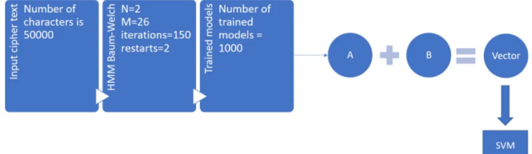
In this technique, the 1000 ciphertexts generated for each of the four classic ciphers, are used as observation sequences to train 1000 HMMs for each category of cipher. These pretrained HMMs are then used as training data for the CNNs. In order to do so, an intermediate step is performed, where the HMM matrices are converted to images. This section discusses the applications of CNNs in cryptanalysis and also discusses the data preparation steps that are followed. 3.3.1 Dataset preparation for CNN

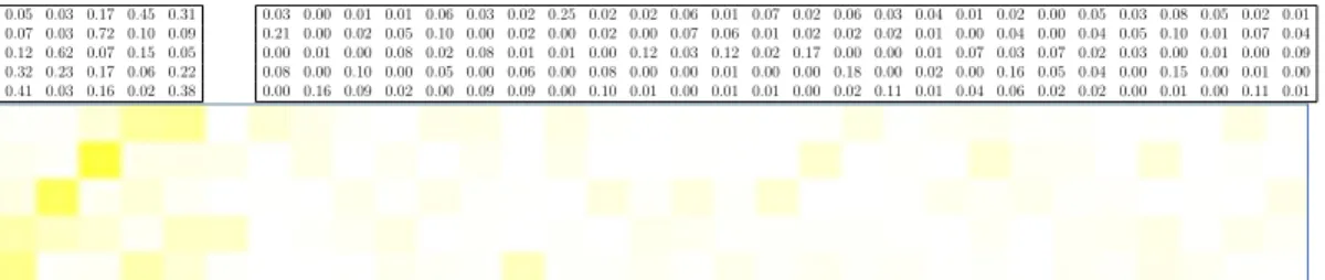
The𝐴 and 𝐵 matrices of HMM are concatenated to a larger matrix and each

matrix is now stored as an image file. Figure 8 shows an example of generated image for HMM trained on simple substitution cipher for 2 hidden states. As seen from Figure 8, the brighter pixels are observed across the diagonals of 𝐴 matrix.

Figure 9 shows an example of generated image for HMM trained on Vigenère cipher for 5 hidden states. As seen from Figure 9 the brighter pixels are observed across the diagonals of 𝐴 matrix as a key of length 5 is used for encrypting the plaintext.

Figure 10 shows the process in which technique 2 is implemented.

0.83 0.17 0.33 0.67

0.13 0.03 0.06 0.07 0.11 0.04 0.02 0.08 0.00 0.00 0.01 0.08 0.04 0.00 0.00 0.03 0.00 0.11 0.11 0.00 0.02 0.00 0.01 0.03 0.00 0.01 0.00 0.00 0.00 0.01 0.28 0.00 0.01 0.00 0.16 0.00 0.00 0.00 0.00 0.00 0.17 0.01 0.00 0.00 0.01 0.18 0.08 0.00 0.05 0.00 0.00 0.02

Figure 8: HMM 𝐴 and 𝐵 matrices converted to image for simple substitution

cipher for 𝑁 = 2 0.05 0.03 0.17 0.45 0.31 0.07 0.03 0.72 0.10 0.09 0.12 0.62 0.07 0.15 0.05 0.32 0.23 0.17 0.06 0.22 0.41 0.03 0.16 0.02 0.38 0.03 0.00 0.01 0.01 0.06 0.03 0.02 0.25 0.02 0.02 0.06 0.01 0.07 0.02 0.06 0.03 0.04 0.01 0.02 0.00 0.05 0.03 0.08 0.05 0.02 0.01 0.21 0.00 0.02 0.05 0.10 0.00 0.02 0.00 0.02 0.00 0.07 0.06 0.01 0.02 0.02 0.02 0.01 0.00 0.04 0.00 0.04 0.05 0.10 0.01 0.07 0.04 0.00 0.01 0.00 0.08 0.02 0.08 0.01 0.01 0.00 0.12 0.03 0.12 0.02 0.17 0.00 0.00 0.01 0.07 0.03 0.07 0.02 0.03 0.00 0.01 0.00 0.09 0.08 0.00 0.10 0.00 0.05 0.00 0.06 0.00 0.08 0.00 0.00 0.01 0.00 0.00 0.18 0.00 0.02 0.00 0.16 0.05 0.04 0.00 0.15 0.00 0.01 0.00 0.00 0.16 0.09 0.02 0.00 0.09 0.09 0.00 0.10 0.01 0.00 0.01 0.01 0.00 0.02 0.11 0.01 0.04 0.06 0.02 0.02 0.00 0.01 0.00 0.11 0.01

Figure 9: HMM 𝐴 and 𝐵 matrices converted to image for Vigenère cipher for

𝑁 = 5

3.4 Training SVMs on pretrained HMMs (technique 3)

In this technique, 1000 trained HMMs for each category of cipher, are considered as features to SVM. In order to do so, an additional step is implemented, where the pretrained HMM matrices are converted to 1D vectors, similar to converting matrices to images as discussed in section 3.3. This section discusses the data preparation steps that are followed for classifying HMMs as vectors.

3.4.1 Dataset preparation for SVM

This step is similar to the dataset preparation step for CNNs, that is mentioned in subsection 3.3.1. The matrices from trained HMMs are converted to a feature vector by appending the probability values of 𝐴 and𝐵 matrices of the HMM to

form a one dimensional vector. Figure 11 shows the process in which the technique 3 is implemented.

CHAPTER 4 Experiments and Results

This section discusses the experimental setup for the techniques implemented in this research. Results for technique 1, that is implemented using SVM are explained in detail followed by technique 2 setup. For technique 2, parameters of HMMs are described and results between CNN and SVM are compared. This research experiments on four classic ciphers namely, simple substitution cipher, Vigenère cipher, column transposition cipher, and playfair cipher.

4.1 Results for technique 1

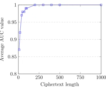
Upon training the SVM for different lengths of ciphertext ranging from 10 to 10000 characters, the results obtained are significantly accurate in comparison to technique 2. Figure 13 shows the increased AUC value as the length of ciphertext trained on increases. Furthermore, it can be observed that, even for a smaller ciphertext of just 10 characters long, SVM gives 0.87 AUC value. Figure A.23 shows converged values of ROC when SVM is trained with ciphertext of 200 characters and more. Figure 12 shows macro-average AUC value for SVM on different lengths of ciphertexts.

4.2 Results for technique 2

To improve CNN's performance, more number of images per cipher type is required. For each cipher category, 1000 HMMs are trained, where each HMM's ciphertext is generated using random key. For this research, two sizes of dataset were generated as shown in Table 14. For each cipher type, different HMMs are trained using parameters shown in Table 15.

CNN is implemented using Keras.Sequential library [28] and

ImageDataGenerator library is used for preprocessing the input images [29].

0 250 500 750 1000 0.8 0.85 0.9 0.95 1 Ciphertext length Average AUC value

Figure 12: SVM macro-average AUC value over different lengths of ciphertexts Table 14: Dataset size

Hidden states Number of HMMs

2, 3, 4 1000 5, 6, 7 200 Table 15: HMM parameters 𝑁 2, 3, 4, 5, 6, 7 𝑇 50000 𝑀 26 Iterations 150 Random restarts 2

epochs [30]. CNN parameters are described in Table 16.

Figure 14 shows that, except for 𝑁 = 5and𝑁 = 2 increasing the number of

Conv2D layers increases the model's training accuracy. This shows that the HMM matrices are more different when, 𝑁 = 2 or if 𝑁 is equal to the key length. Hence

the images can be differentiated with less number of convolution layers [31]. Figure 15 shows the confusion matrix values when CNN is trained on different

(a) Length of ciphertext 10 (b) Length of ciphertext 20

(c) Length of ciphertext 40 (b) Length of ciphertext 50

(d) Length of ciphertext 70 (e) Length of ciphertext 90 Figure 13: ROC plots for SVM trained on different lengths of ciphertext

𝑁 values including 2, 4, 5, 7. As seen in Figure 15, the normalized confusion matrix

for 𝑁 = 2 and 𝑁 = 4 shows non-significant results and the classification accuracy

is low. However, for 𝑁 = 5 and 𝑁 = 7, most of the playfair cipher is classified as

Vigenère cipher. The reason is the key length used for both playfair and Vigenère ciphers, which is exactly 5. Hence, for 𝑁 = 5 and𝑁 = 7 the HMMs are not that

Table 16: CNN parameters Image dimensions 𝑁 ×(𝑁 + 26) Batch size 32 Conv2D layers 2, 3, 4 Max-pooling layers 2, 3 Epochs 100

Steps per epoch 10

Loss function layers categorical cross entropy

Optimizer Adam-optimizer 2 3 4 5 6 7 0.4 0.5 0.6 0.7 0.8 0.9 1 0 . 83 0 . 9 0 . 87 0 . 92 0 . 91 0 . 97 0 . 74 0 . 91 0 . 88 0 . 86 0 . 92 0 . 98

Number of hidden states

CNN

model’s

training

accuracy

2 Conv2D layers 3 Conv2D layers

Figure 14: CNN model training accuracy for 2 and 3 Con2D layers

different for these two ciphers. This can be seen from Figure 16, where playfair cipher and Vigenère ciphers have similar patterns of brighter pixels in sub-grids of images.

Figure A.25 shows that CNNs are unable to clearly differentiate between ciphers, when they are considered as images. The images obtained from HMMs could have similar levels of brighter pixels in various parts of the matrix even though the ciphertext is different. Furthermore, most of the image regions are lighter indicating a probability of 0 value in HMM matrix. The maximum average AUC value is obtained for 𝑁 = 5 and 𝑁 = 7, because of the length of the key

(a) 𝑁 = 2 (b) 𝑁 = 4

(d) 𝑁 = 5 (e) 𝑁 = 7

Figure 15: Confusion matrix plots for CNN having two Conv2D layers for 𝑁 as

2,4,5,7

used for Vigenère and playfair ciphers. Thus, making it easier for the CNN to distinguish.

4.3 Results for technique 3

SVM is implemented using same approach as mentioned in Section 4.1. For

𝑁 = 2, Figure 17 shows the confusion matrix of SVM trained on 1000 feature

vectors from each of the four HMM types. This confusion matrix is calculated after 10-fold cross validation. Figure 18 shows the corresponding ROC plot showing accuracies for each individual cipher type along with micro and macro-average AUC values for multi-class classification [31].

(a) HMM images for Vigenère and playfair 𝑁 = 5

(b) HMM images for Vigenère and playfair 𝑁 = 7

Figure 16: Converged HMM images for Vigenère and playfair ciphers for 𝑁 = 5

and 𝑁 = 7

Figure 17: Confusion matrix for 𝑁 = 2

When 𝑁 = 5, Figure 19 shows the confusion matrix of SVM trained on

200 feature vectors from each of the four HMM types. This confusion matrix is calculated after 10-fold cross validation. Figure 20 shows the corresponding

Figure 18: ROC for𝑁 = 2

ROC plot showing accuracies for each individual cipher type along with micro and macro-average AUC values for multi-class classification [31].

Figure 19: Confusion matrix for 𝑁 = 5

On comparing the number of miss-classifications of Vigenère as playfair and vice-versa from Figure 19, we can observe that this value increases when number of hidden states approaches 5. The reason being the key length used to encrypt

Figure 20: ROC for𝑁 = 5

Vigenère and playfair cipher is 5. Hence, for𝑁 = 5, the HMM is not that different

for these two ciphers. Therefore, the SVM miss-classifies more when 𝑁 value is

closer to 5. Vigenère and playfair ciphers can be thought of being more similar because, Vigenère encryption algorithm substitutes blocks of plaintext message, like the playfair which follows a digraph substitution. Hence the frequencies of individual letters of plaintext changes completely after encryption and is not substituted like in case of simple substitution cipher.

From Figure 18 and Figure 20 we can see that, for 𝑁 = 2 and 𝑁 = 5, the

LinearSVC classifier is able to distinguish four classes of cipher with an average accuracy of at least 0.98 [32]. Figure 21 and Figure 22 shows that as 𝑁 increases,

there is a decrease in the number of simple substitution HMM samples incorrectly classified as column transposition HMM. Intuitively, simple substitution encryption can be considered as shift of 26 letters among each other in the English alphabet. The same logic can be applied to column transposition cipher encryption, as the letters are just permuted among each other. Hence, the SVM is not able to clearly distinguish between HMMs that were modelled on simple substitution cipher and

column transposition cipher. However, the key length used to encrypt column transposition cipher is 5. Therefore, as 𝑁 approaches 5 the converged HMM values

for column transposition and simple substitution differ, making it easier for the SVM model to correctly classify.

(a) 𝑁 = 2 (b) 𝑁 = 3

(c) 𝑁 = 4

Figure 21: Confusion matrix grid for SVM trained on 1000 HMMs for each of the four cipher classes

Table 17 shows results of three techniques implemented in this research. Technique 1 and technique 3 perform better when compared to technique 2. Between technique 1 and 3, we can see that, technique 3 gives a much clearer classification with fewer number of data points. Meaning, the minimum length of input training sample required for technique 3 is less than length required for technique 2. The

(a) 𝑁 = 6 (b) 𝑁 = 7

(c) 𝑁 = 5

Figure 22: Confusion matrix grid for SVM trained on 200 HMMs for each of the four cipher classes

maximum AUC value is obtained in technique 3 for 𝑁 = 5. After combining 𝐴

and 𝐵 matrices of the HMM, a 155 length input vector is obtained which serves as

the feature vector for SVM. Hence, we can conclude that, HMMs when combined with SVMs outperforms rest of the techniques.

Table 17: Results of three techniques Technique Minimum length of

training sample Minimum numberof training samples per class Maximum AUC value Technique 1 200 200 1.00 Technique 2 155 200 0.71 Technique 3 155 200 1.00

CHAPTER 5 Conclusion

Given a ciphertext message, this research detects the type of classic cipher algorithm used to encrypt its corresponding plaintext message. We approach this problem in two ways. Firstly, ciphertext themselves are classified without considering any alternative features. However, intuitively we would assume that any ciphertext alone does not imply much significant meaning. Hence, in the second approach, this research initially applies a discrete hill-climb machine learning technique, that is, HMM, to capture hidden statistical dependencies between letters of the ciphertext. These statistical values are then used to determine the underlying ciphertext, thereby making the detection process much more effective and consistent.

Under the first approach, we experiment on SVMs, whose input feature vectors are ciphertexts of varied lengths (technique 1). This research agrees that technique 1 proves to be a relatively accurate solution for classification. The results of this technique disproves the initial assumption in this research, about stand-alone ciphertexts not containing distinguishable features. Under the second approach, CNNs (technique 2) and SVMs (technique 3) are used to classify the HMMs. Comparison of performance results show that SVM performs significantly better in both technique 1 and technique 3 with an average accuracy of 0.99.

Referring to Figure 21, we can see the significant decrease in number of miss-classifications between simple substitution and column transposition. One interesting approach would be to determine the unknown key length. This can be implemented by experimenting with different number of hidden states of HMM and classifying against an already trained SVM or CNN. The 𝑁 value that has the least

used. Furthermore, experimenting with 𝑁 = 26, could give better differentiation

between playfair and Vigenère cipher, because, playfair cipher's digraph statistics would follow English language's digraph statistics, unlike Vigenère's. Another approach would be to use converged 𝐴 and 𝐵 matrices separately, because, for

certain ciphers, the 𝐵 matrix does not provide useful information. Considering

individual matrices would help in a more accurate classification by eliminating non-significant features. This would also mean that minimal data would suffice in performing an effective classification. More such types of ciphers, such as double transposition ciphers, could be experimented with, as they are not entirely straightforward. Furthermore, it would be interesting to use and test these models for scoring different types of encryption algorithms including modern ciphers.

Recently, a controversial solution to the Zodiac 340 (Z340) cipher has been proposed [33]. This problem provides an ideal opportunity to score the Z340 cipher against these trained models and identify which classic cipher it would correspond to.

The scope of this research can also be extended to implementing transfer learning from neural networks for cryptanalysis. This innovative approach relies on ways to store models trained for one problem and applying solutions on a different one [20]. This efficient technique can be implemented using online algorithms. Using an online HMM [20], to implement transfer learning on more classes of ciphers, could also be one of the future scopes of this research.

LIST OF REFERENCES

[1] M. Stamp, ‘‘A revealing introduction to hidden Markov models,’’ https:// www.cs.sjsu.edu/~stamp/RUA/HMM.pdf, 2004.

[2] C. Wang, ‘‘Convolutional neural network for image classification,’’ 2015, [Online; accessed April 21, 2019]. [Online]. Available: https://pdfs. semanticscholar.org/b8e3/613d60d374b53ec5b54112dfb68d0b52d82c.pdf [3] H. Kandan, ‘‘Understanding the kernel trick,’’ 2017, [Online; accessed April

21, 2019]. [Online]. Available: https://towardsdatascience.com/understanding-the-kernel-trick-e0bc6112ef78

[4] P. Saimadhu, ‘‘Svm classifier implementation in python with scikit-learn,’’ 2017, [Online; accessed April 21, 2019]. [Online]. Available: http://dataaspirant. com/2017/01/25/svm-classifier-implemenation-python-scikit-learn/

[5] M. Stamp, Information Security: Principles and Practice. Wiley, 2011.

[6] K. David, The Codebreakers. Scribner, 1997.

[7] A. Dhavare, R. Low, and M. Stamp, ‘‘Efficient cryptanalysis of homophonic substitution ciphers,’’ Cryptologia, vol. 37, no. 3, pp. 250--281, July 2013.

[Online]. Available: http://dx.doi.org/10.1080/01611194.2013.797041

[8] M. Stamp, F. Di Troia, M. Stamp, and J. Huang, ‘‘Hidden markov models for vigenère cryptanalysis,’’ in Proceedings of the 1st International Conference on Historical Cryptology HistoCrypt 2018, 2018, pp. 39--46.

[9] C. K. Shene, ‘‘The vigenère cipher encryption and decryption,’’ https://pages. mtu.edu/~shene/NSF-4/Tutorial/VIG/Vig-Base.html, [Online; accessed April 21, 2019].

[10] S. Khan, ‘‘Design and analysis of playfair ciphers with different matrix sizes,’’

International Journal of Computing and Network Systems, vol. 3, pp. 117

--122, September 2015.

[11] S. Baragada and P. Satyanrayana Reddy, ‘‘A survey on machine learning approaches to cryptanalysis,’’ International Journal of Emerging Trends and Technology in Computer Science (IJETTCS), vol. 2, 2013.

[12] P. Kumar Ray, S. Kant, B. Roy, and A. Basu, ‘‘Classification of encryption algorithms using the hidden markov model,’’ Calcutta Statistical Association Bulletin, vol. 64, pp. 277--290, September 2012.

[13] P. Kumar Ray, S. Ojha, B. Kumar Roy, and A. Basu, ‘‘Classification of encryption algorithms using fisher’s discriminant analysis,’’ Defence Science Journal, vol. 67, p. 59, December 2016.

[14] G. Sivagurunathan, V. Rajendran, and T. Purusothaman, ‘‘Classification of substitution ciphers using neural networks,’’International Journal of Computer Science and Network Security, April 2019.

[15] A. Jacovi, O. S. Shalom, and Y. Goldberg, ‘‘Understanding convolutional neural networks for text classification,’’ CoRR, vol. abs/1809.08037, 2018.

[Online]. Available: http://arxiv.org/abs/1809.08037

[16] A. Chavda, K. Potika, F. Di Troia, and M. Stamp, ‘‘Support vector machines for image spam analysis,’’ in ICETE, January 2018, pp. 597--607.

[17] D. Rajeswaran, F. Di Troia, T. Austin, and M. Stamp, Function Call Graphs Versus Machine Learning for Malware Detection: An Artificial Intelligence

Approach. Springer, September 2018, pp. 259--279.

[18] Anna University, ‘‘Classification of classical substitution ciphers,’’ [Online; accessed April 21, 2019]. [Online]. Available: http://shodhganga.inflibnet.ac. in/bitstream/10603/141410/11/11_chapter%203.pdf

[19] R. Vobbilisetty, F. D. Troia, R. M. Low, C. A. Visaggio, and M. Stamp, ‘‘Classic cryptanalysis using hidden Markov models,’’ Cryptologia, vol. 41,

no. 1, pp. 1--28, 2017. [Online]. Available: https://doi.org/10.1080/01611194. 2015.1126660

[20] M. Stamp, ‘‘Deep thoughts on deep learning,’’ San Jose State University,

2018. [Online]. Available: https://www.cs.sjsu.edu/~stamp/ML/files/ann.pdf [21] E. W. Weisstein, ‘‘Convolution from mathworld - a wolfram web resource,’’

http://mathworld.wolfram.com/Convolution.html, accessed: 2019-04-21. [22] A. Khan, A. Sohail, U. Zahoora, and A. S. Qureshi, ‘‘A survey of the

recent architectures of deep convolutional neural networks,’’ CoRR, vol.

abs/1901.06032, 2019. [Online]. Available: http://arxiv.org/abs/1901.06032 [23] T. Guo, J. Dong, H. Li, and Y. Gao, ‘‘Simple convolutional neural network

on image classification,’’ in 2017 IEEE 2nd International Conference on Big Data Analysis (ICBDA), March 2017, pp. 721--724.

[24] J. Suriya Prakash, K. Annamalai Vignesh, C. Ashok, and R. Adithyan, ‘‘Multi class support vector machines classifier for machine vision application,’’ in2012 International Conference on Machine Vision and Image Processing (MVIP),

[25] R. Gandhi, ‘‘Support vector machine - introduction to machine learning algorithms,’’ 2018, [Online; accessed April 21, 2019]. [Online]. Avail-able: https://towardsdatascience.com/support-vector-machine-introduction-to-machine-learning-algorithms-934a444fca47

[26] scikit-learn, ‘‘Stratified k-fold classifier,’’ [Online; accessed April 21, 2019]. [Online]. Available: https://scikit-learn.org/stable/modules/generated/ sklearn.model_selection.StratifiedKFold.html

[27] scikit-learn, ‘‘Onevsrest classifier,’’ [Online; accessed April 21, 2019]. [Online]. Available: https://scikit-learn.org/stable/modules/generated/ sklearn.multiclass.OneVsRestClassifier.html

[28] keras, ‘‘Keras sequential library,’’ [Online; accessed April 21, 2019]. [Online]. Available: https://keras.io/models/sequential/

[29] keras, ‘‘Imagedatagenerator,’’ [Online; accessed April 21, 2019]. [Online]. Available: https://keras.io/preprocessing/image/

[30] keras callbacks, ‘‘Keras callbacks checkpoint,’’ [Online; accessed April 21, 2019]. [Online]. Available: https://keras.io/callbacks/

[31] scikit-learn, ‘‘Receiver operating characteristic (roc) for multiclass setting,’’ [Online; accessed April 21, 2019]. [Online]. Available: https://scikit-learn.org/stable/auto_examples/model_selection/plot_roc.html

[32] scikit-learn, ‘‘Linearsvc classifier,’’ [Online; accessed April 21, 2019]. [Online]. Available: https://scikit-learn.org/stable/modules/generated/sklearn.svm. LinearSVC.html

[33] M. Stamp, ‘‘Is this the Zodiac speaking?’’ [Personal Correspondence: www.cs. sjsu.edu/~stamp/], 2018.

APPENDIX Appendix A A.1 Results for technique 1

Referring to Table 7 the following results are obtained for technique 1.

(f) Length of ciphertext 100 (g) Length of ciphertext 200

(h) Length of ciphertext 300 (i) Length of ciphertext 400

(j) Length of ciphertext 500 (k) Length of ciphertext 1000 Figure A.23: ROC plots for SVM trained on different lengths of ciphertext A.2 Results for technique 3

(a) 𝑁 = 2 (b) 𝑁 = 3

(c) 𝑁 = 4 (b) 𝑁 = 5

(d) 𝑁 = 6 (e) 𝑁 = 7

Figure A.24: ROC plots for SVM trained on 200 HMMs for each of the four cipher classes

A.3 Results for technique 2

(a) 𝑁 = 2 (b) 𝑁 = 3

(c) 𝑁 = 4 (b) 𝑁 = 5

(d) 𝑁 = 6 (e) 𝑁 = 7

A.3.2 Confusion matrix plots for CNN having two convolution layers

(a) 𝑁 = 2 (b) 𝑁 = 3

(c) 𝑁 = 4 (b) 𝑁 = 5

(d) 𝑁 = 6 (e) 𝑁 = 7

A.3.3 ROC plots for CNN having three convolution layers

(a) 𝑁 = 2 (b) 𝑁 = 3

(c) 𝑁 = 4 (b) 𝑁 = 5

(d) 𝑁 = 6 (e) 𝑁 = 7

A.3.4 Confusion matrix plots for CNN having three convolution layers

(a) 𝑁 = 2 (b) 𝑁 = 3

(c) 𝑁 = 4 (b) 𝑁 = 5

(d) 𝑁 = 6 (e) 𝑁 = 7

Figure A.28: Confusion matrix plots for CNN having three Conv2D layers A.4 Vigenère cipher key table

A B C D E F G H I J K L M N O P Q R S T U V W X Y Z 0 0 B C D E F G H I J K L M N O P Q R S T U V W X Y Z A 1 1 C D E F G H I J K L M N O P Q R S T U V W X Y Z A B 2 2 D E F G H I J K L M N O P Q R S T U V W X Y Z A B C 3 3 E F G H I J K L M N O P Q R S T U V W X Y Z A B C D 4 4 F G H I J K L M N O P Q R S T U V W X Y Z A B C D E 5 5 G H I J K L M N O P Q R S T U V W X Y Z A B C D E F 6 6 H I J K L M N O P Q R S T U V W X Y Z A B C D E F G 7 7 I J K L M N O P Q R S T U V W X Y Z A B C D E F G H 8 8 J K L M N O P Q R S T U V W X Y Z A B C D E F G H I 9 9 K L M N O P Q R S T U V W X Y Z A B C D E F G H I J 10 10 L M N O P Q R S T U V W X Y Z A B C D E F G H I J K 11 11 M N O P Q R S T U V W X Y Z A B C D E F G H I J K L 12 12 N O P Q R S T U V W X Y Z A B C D E F G H I J K L M 13 13 O P Q R S T U V W X Y Z A B C D E F G H I J K L M N 14 14 P Q R S T U V W X Y Z A B C D E F G H I J K L M N O 15 15 Q R S T U V W X Y Z A B C D E F G H I J K L M N O P 16 16 R S T U V W X Y Z A B C D E F G H I J K L M N O P Q 17 17 S T U V W X Y Z A B C D E F G H I J K L M N O P Q R 18 18 T U V W X Y Z A B C D E F G H I J K L M N O P Q R S 19 19 U V W X Y Z A B C D E F G H I J K L M N O P Q R S T 20 20 V W X Y Z A B C D E F G H I J K L M N O P Q R S T U 21 21 W X Y Z A B C D E F G H I J K L M N O P Q R S T U V 22 22 X Y Z A B C D E F G H I J K L M N O P Q R S T U V W 23 23 Y Z A B C D E F G H I J K L M N O P Q R S T U V W X 24 24 Z A B C D E F G H I J K L M N O P Q R S T U V W X Y 25 25