A General Forecast-error Taxonomy

David F. Hendry∗ Nuffield College,

Oxford. January 26, 2000

Abstract

We consider the sources of forecast errors and their consequences in an evolving economy sub-ject to structural breaks,forecasting from mis-specified, data-based models. A model-free taxonomy of forecast errors highlights that deterministic shifts are a major cause of systematic forecast failure. Other sources seem to pose fewer problems. The taxonomy embeds several previous model-based taxonomies for VARs, VECMs, and multi-step estimators, and reveals the stringent requirements that rationality assumptions impose on economic agents.

1 Introduction

Economies regularly undergo institutional, political, financial, and technological changes. Recent ex-amples include the abolition of exchange controls, financial liberalization, the European Union, and privatization. Such changes induce non-stationarities in data processes, and when relatively sudden, can manifest themselves as structural breaks in econometric models, leading to forecast failure, defined as a significant deterioration in forecast performance relative to the anticipated outcome. Empirical ex-amples of serious forecast failure in the UK include missing the stagflation of the 1970s, the consumer boom of the mid 1980s, and the depth of the recession in the early 1990s.

Econometric forecasting models comprise three main components: deterministic terms (e.g., for intercepts and trends), with known future values; observed stochastic variables with unknown future values; and unobserved errors all of whose values (past, present and future) are unknown, though per-haps estimable in the context of a model. Any of these components, or the relationships between them, could be inappropriately formulated, inaccurately estimated, or change in unanticipated ways. All nine types of mistake could induce poor forecast performance, either from inaccurate (i.e., biased), or im-precise (i.e., high variance) forecasts. but Clements and Hendry (1998a, 1999a) find that some mistakes have pernicious effects on forecasts, whereas others are relatively less important. Their theory provides a basis for interpreting, and potentially circumventing, systematic forecast failure in economics, and reveals that many of the conclusions established for correctly-specified forecasting models of constant-parameter processes no longer hold. No forecasting methods fare well when unanticipated breaks occur

after forecasts are announced, and absent pre-cognition, no such methods seem possible. However,

real-time forecasts are eventually made after breaks have occurred, and then some methods are more robust than others.

Since forecast failure has often occurred, to be relevant for economic forecasting, a theory must commence from non-stationary data generation processes (DGPs), specifically, mechanisms that are not

∗_{Financial support from the UK Economic and Social Research Council under grant L116251015 is gratefully} acknowledged.

reducible to stationarity after differencing, cointegration, and possibly co-breaking, transforms. While Clements and Hendry (1998a, 1999a) allow for a non-stationary economy, measured by inaccurate data, using forecasting models which are mis-specified in unknown ways, and possibly incorrectly selected and estimated, the bulk of their analysis is in the context of vector autoregressions (VARs) and vec-tor equilibrium-correction models (VECMs) subject to structural breaks. Here we consider the generic sources of error that might be detrimental to the forecasting enterprise, in terms of both their sources and likely impacts, by deriving a general taxonomy of forecast errors. This embeds several previous model-based taxonomies for VARs, VECMs, and multi-step estimators: simulation results and an empirical example are provided in Hendry (1999) and Clements and Hendry (1998b) respectively. To make the analysis more operational, we relate it to taxonomies for a VECM and VARs in first and second differ-ences (DV and DDV respectively: see Clements and Hendry, 1995), focusing on forecast-error biases and variances. The last two models are more robust to breaks, but we note some ‘tricks’ that can mimic much of that benefit in a VECM. We also briefly discuss whether other mistakes in modelling could account for forecast failure, especially the impact of data-based selection.

In addition, the taxonomy reveals the stringent requirements that rationality assumptions impose on economic agents seeking to anticipate future outcomes in such a non-stationary environment. Agents must not only know all the relevant information, but also how every item of information enters the joint data density at every point in time – including the future – when many of the events involved are unanticipatable. Indeed, when a model differs from a non-constant generating mechanism, the basic theorem that forecasting based on causal variables will dominate that using non-causal cannot be proved: see Clements and Hendry (1998a). As it is unwise to use model-based expectations, when models are manifestly mis-specified, ‘sensible’ agents might learn that they cannot form expectations any better than the best ‘robust forecasting rules’.

The structure of the paper is as follows. Section 2 describes the sources of forecast failure, and presents a model-free taxonomy of forecast errors in section 3. This is fleshed out for a VAR in section 4. Section 5 compares its implications for the forecast-error biases and variances of a VECM, DV and DDV. As one of the implications of the taxonomy, section 6 reviews the detectability of breaks. Section 7 notes the possible effects of data-based selection, and the use of forecast performance to select models. Section 8 considers approaches to modelling or removing deterministic shifts. Finally, section 9 draws some implications for models of expectations formations, and section 10 concludes.

2 Sources of forecast failure

The possible sources of mistakes that can induce multi-step forecast errors from econometric models of possibly cointegratedI(1) processes can be delineated in a formal taxonomy. This highlights which sources induce forecast-error biases, and which have variance effects. The framework comprises:

(1) a forecasting model formulated in accordance with some theoretical notions, (2) selected by some empirical criteria,

(3) but mis-specified (to an unknown extent) for the DGP, (4) with parameters estimated (possibly inconsistently), (5) from (probably inaccurate) observations,

(6) which are generated by an integrated-cointegrated process, (7) subject to intermittent structural breaks.

Such assumptions more closely mimic the empirical setting than those often underlying investigations of economic forecasting, and we explored this framework in detail in Clements and Hendry (1998a, 1999a).

The resulting forecast-error taxonomy includes a source for the effects of each of 2.–7., partitioned (where appropriate) for deterministic and stochastic influences: see 3.

Our analysis utilizes the concepts of a DGP and a model thereof, and attributes the major problems of forecasting to structural breaks in the model relative to the DGP. Between the actual DGP and the empirical forecasting model, there lies a ‘local DGP of the variables being modelled’, denoted the LDGP: see Bontemps and Mizon (1996). Using a VECM as the DGP in a two-tier system (say) entails that the VECM is the LDGP in the three-tier stratification. Changes in growth rates or equilibrium means in the VECM could be viewed as resulting from a failure to model the forces operative at the level of the DGP. The correspondence between the LDGP and DGP is assumed to be close enough to sustain an analysis of forecasting, checked by what happens in practice (via empirical illustrations, where the outcomes depend on the actual, but unknown, mapping between the forecasting model and the economy). We first formalize the DGP and the forecasting models, then record the taxonomy of forecast errors, before focusing on the biases and variances of the various models.

3 A general forecast-error taxonomy

Consider a vector of n stochastic variables {x_t}, where the joint density of x_t at time t is

D_xt[x_t|X1_t−1,q_t], conditional on information X1_t−1 = (x₁. . .x_t−1) available at the time, when

q_t denotes the relevant deterministic factors (such as intercepts, trends, and indicators). Because the underlying densities may be changing over time, all expectations operators must be time dated. It is de-sired to forecast a function ofx_T+h, such as itself, or perhaps the non-integrated components (denoted

{y_T+h}below) over forecast horizons h = 1, . . . , H, from a forecast origin atT. A dynamic model

M_xt[x_t|Xt_t−₋s₁,qe_t,θ_t], with deterministic terms eq_t, lag length s, and implicit stochastic specification defined by its parameters θ_t, is fitted over the sample t = 1, . . . , T to produce a forecast sequence

{bx_T+h|T}. Parameter estimates are a function of the observables, represented by:

b θT =fT

e

X1_T,Qe1_T, (1)

whereXe denotes the measured data. The subscript onbθin (1) represents the influence of sample size, whereas that onθ_tinM_xt[·]denotes that the derived parameters may alter over time (perhaps reflected in changed estimates). Letθ_e,T =E_T[bθ_T](where that exists).

Since future values of the deterministic terms are known, but those of stochastic variables are un-known: b x_T+h|T =g_hXeT−s+1 T ,qeT+h,bθT . (2)

In (2),XeT_T−s+1enters up to the forecast origin, which might be less well measured than earlier data: see e.g., Wallis (1993).1 Forecast accuracy is to be judged by a criterion functionC e_T+1|T. . .e_T+H|T, which we take to depend only on the forecast errorse_T+h|T =x_T+h−bx_T+h|T, where ‘smaller’ values ofC(·)are preferable. Because the model will generally be a mis-specified representation of the LDGP, a different expectations operator, E[·], is used to denote expectations based on the estimated model, so that: ET h x_T+h|XeT−s+1 T ,eqT+h,bθT i =ET+h h b x_T+h|T |XeT−s+1 T ,qeT+h,bθT i . (3)

It is easiest to understand (3) by a Monte Carlo analogy: using (2), the average forecast value that results is given by the right-hand side of (3). Thus,E_T[·]denotes the mean forecast forx_T+h from the model

1_{The dependence of}bθ

usingbθ_T estimated overt= 1, . . . , T. The expected forecast error that eventuate is, however: ET+h h e_T+h|T |X1 T,{Q∗}1T+h i =ET+h h x_T+h−bx_T+h|T|X1 T,{Q∗}1T+h i (4)

where the actual values of the deterministic factors over the forecast period (incorporating any determ-inistic shifts), are denoted by{Q∗}T_T+1_+hand[Q1_T,{Q∗}T_T+1_+h] ={Q∗}1_T+h.

Equation (4) is the expression of central importance to our explanation of forecast failure. Let:

ε_T+h|T =x_T+h−ET+h h x_T+h |X1 T,{Q∗}1T+h i , (5)

be theh-steps ahead LDGP forecast error from an origin atT. By construction,E_T+h[ε_T+h|T|X1_T,{Q∗}1_T+h] =

0, so ε_T+h|T is an innovation against all available information. Indeed, under ‘rational expecta-tions’, ε_T+h|T in (5) is precisely the forecast error that would result ex post. However, even for correctly-observed sample data – assumed hereafter – so that Xe1_T−s = X1_T−s, it is not the case that

ET+h[eT+h|T|X1T,{Q∗}1T+h]6=0in general, as we now show.

The forecast errore_T+h|T =x_T+h−xb_T+h|T from the modelM_T[x_T+h|XeT_T−s+1,eq_T+h,θb_T]can be decomposed as: ET+h h x_T+h |X1 T,{Q∗}1T+h i −ET+hxT+h |X1T,Q1T+h (ia) + ET+hxT+h|X1T,Q1T+h −ETxT+h |X1T,Q1T+h (ib) +ET xT+h|X1T,Q1T+h −ET h x_T+h |X1 T,Qe1T+h i (iia) +ET h x_T+h|X1 T,Qe1T+h i − ET h x_T+h|X_TT−s+1,eq_T+h,θe,T i (iib) +ET h x_T+h |XT_T−s+1,eq_T+h,θe,T i − ET h x_T+h|Xe_TT−s+1,eq_T+h,θe,T i (iii) +ET h x_T+h |Xe_TT−s+1,eq_T+h,θe,T i −bx_T+h|T (iv) +ε_T+h|T. (v) (6)

The first two rows arise from structural change affecting deterministic (ia) and stochastic (ib) compon-ents respectively; the third and fourth, (iia) and (iib), from model mis-specification decomposed by deterministic and stochastic elements; the fifth (iii) from forecast-origin inaccuracy; the sixth (iv) from estimation uncertainty, and the last row from the inherent stochastic nature of economies.

When{Q∗}T_T+1_+h =QT_T+1_+h(so there are no deterministic shifts), then (ia) is zero; and in general, the converse holds, that (ia) being zero entails no deterministic shifts. WhenE_T+h[·] =E_T [·](so there are no stochastic breaks), (ib) is zero; but (ib) can be zero despite stochastic breaks, providing these do not indirectly alter deterministic terms. When the deterministic terms in the model are correctly specified, so Q1_T+h = Qe1_T+h then (iia) is zero, and again the converse seems to hold. For correct stochastic specification, soθ_e,Tsummarizes the effects ofX1_T, then (iib) is zero but now the converse is false – (iib) can be zero in seriously mis-specified models. Next, when the data are accurate (especially important at the forecast origin), soXe =X, (iii) is zero, but the converse is not entailed. When estimated parameters have zero variances, sobx_T+h|T =E_T[x_T+h|·,θ_e,T], then (iv) is zero, and conversely (except for events of probability zero). Finally, (v) is zero if and only if the world is non-stochastic.

Thus, the taxonomy in (6) includes elements for the main sources of forecast error, partitioning these by whether or not the corresponding expectation is zero. Its application to the forecast errors from a VAR is discussed in the next section. Non-zero expectations entail systematic forecast errors, whereas zero-expectation effects only influence higher moments. This suggests that the former will be easier to detect than the latter, and that is the focus of section 6. If models represent an LDGP with

no deterministic terms, then we anticipate that they will be more robust to breaks: that is the topic of section 5, where DV and DDV models are shown to be more robust after breaks than VECMs. We return in section 9 to consider its implications for models of expectation formation.

4 The taxonomy for a VAR

To illustrate (6) more concretely, consider a first-order vector autoregressive DGP which is stationary in-sample (perhaps after appropriate cointegration and differencing transformations):

y_T+h =φ+Πy_T+h−1+T+h,

with_t∼IN_n[0,Ω]using the forecasting model:

b

y_T+h =φb+Πyb _T+h−1.

The unconditional mean ofy_tis:

E[y_t] = (I_n−Π)−1φ=ϕ (7) and hence, in deviations:

y_t−ϕ=Π(y_t−1−ϕ) +t.

Theh-step ahead forecasts at timeT forh = 1, . . . , Hcan be written as:

b

y_T+h−ϕb =Πb (yb_T+h−1−ϕb) =Πbh(by_T −ϕb), (8) whereϕb = (I_n−Πb)−1φb, and ‘∧’s denote estimates on parameters, and forecasts on random variables. Although initial conditions are unknown in practice, we assumeE[yb_T] =ϕhere, so that on average no systematic bias results from data inaccuracy.

After the forecasts have been made at timeT,(φ:Π)change to(φ∗ :Π∗), whereΠ∗ still has all its eigenvalues less than unity in absolute value, so the process remainsI(0). Then, fromT+ 1onwards, the data are generated by:

y_T+h = φ∗_+Π∗_y T+h−1+T+h = ϕ∗+Π∗(y_T+h−1−ϕ∗) +T+h = ϕ∗_{+ (Π}∗₎h_(y T −ϕ∗) + h−1 X i=0 T+h−i,

so both the slope and the intercept alter. Letb_T+h|T =y_T+h−yb_T+h|T, then the forecast-error taxonomy becomes (the matricesC_h andF_h are complicated functions of the whole-sample data, the method of estimation, and the forecast-horizon – see e.g., Calzolari, 1981 –(·)ν denotes column vectoring, and the subscriptpdenotes a plim):

VAR forecast-error taxonomy

b

T+h|T '

I_n−(Π∗₎h_(ϕ∗_{−ϕ) (ia) equilibrium-mean change}

+(Π∗₎h_−Πh_(y

T −ϕ) (ib) slope change

+ I_n−Πh p

ϕ−ϕp (iia) equilibrium-mean mis-specification

+ Πh_−Πh

p(yT −ϕ) (iib) slope mis-specification

− Πh

p +Ch(yT −ybT) (iii) forecast-origin uncertainty

− I_n−Πh

p(ϕb−ϕ) (iva) equilibrium-mean estimation

−F_hΠb −Πν (ivb) slope estimation

+hX−1

i=0

(Π∗₎i

T+h−i (v) error accumulation.

(9)

In (9), terms involving y_T −ϕhave zero expectations even under changed parameters (e.g., (ib) and (iib)). Moreover, for symmetrically-distributed shocks, biases inΠb forΠwill not induce biased fore-casts (see e.g., Clements and Hendry, 1998a), and the_T+h have zero means by construction. Con-sequently, the primary sources of systematic forecast failure are (ia), (iia), (iii), and (iva). However, on ex post evaluation, (iii) will be removed, and in congruent models with freely-estimated intercepts, (iia) and (iva) will be zero on average. That leaves (ia) as the primary source. We now consider these implications in more detail, commencing with mean effects, then turn to variance components.

4.1 Mean effects

The key effect derives from changes to the ‘equilibrium mean’ ϕ (not necessarily the intercept φ in a model, as seen in (9)), namely the unconditional expectation E[y_t] (where that exists) of the non-integrated components of the vector of variables under analysis. Consequently, E_T+h[y_T+h]−

ET[yT+h] is the major determinant of systematic forecast failure. In non-stationary dynamic

pro-cesses, where unconditional expectations may not be defined, this expression can be generalized to

ET+h[xT+h|XT]− ET[xT+h|XT]where X_T denotes observations up to and including the forecast origin.

The admissible deductions on observing either the presence or absence of forecast failure are rather stark, particularly for general methodologies which believe that forecasts are the appropriate way to judge empirical models. In this setting of structural change in deterministic components, there may exist non-causal models (i.e., models none of whose ‘explanatory’ variables enter the DGP) that do not suffer forecast failure, and indeed may forecast absolutely more accurately on reasonable measures, than previously congruent, theory-based, efficiently-estimated econometric models: example are provided in Hendry (1997), Clements and Hendry (1999a) and section 5. Consequently, even relative success or failure is not a reliable basis for selecting between models – other than for forecasting purposes. Conversely, a model that suffers severe forecast failure may nonetheless have constant parameters on

ex post re-estimation: apparent failure on forecasting need have no implications for the goodness of a

model, or its theoretical underpinnings, as it may arise from incorrect data, that are later corrected (see the concept of extended constancy in Hendry, 1996).

Mis-specification of zero-mean stochastic components is unlikely to be a major source of forecast failure, but stochastic mis-specification could involve deterministic mis-specification, which might

in-teract with deterministic breaks elsewhere in the economy, and thereby precipitate failure. Equally, the false inclusion of variables which experience equilibrium-mean shifts could have a marked im-pact on forecast failure: the model mean would shift although the data mean did not, thereby changing

ET[yT+h], whenET+h[yT+h]was unaltered. Finally, forecast-origin mis-measurement can also be

per-nicious, as an incorrect starting level is ‘carried forward’ in dynamic models – hence most forecasting agencies carefully appraise the latest observations for consistency with other available information.

4.2 Variance effects

Compared to the problems of the previous section, estimation uncertainty for the parameters of stochastic variables seems a secondary problem, as such errors add variance terms of O(1/T) for stationary components – and O(1/T2) for non-stationary – for samples of size T. However, mis-estimation of coefficients of deterministic terms could be deleterious to forecast accuracy when

ET+h[yT+h]−ET\[yT+h]is large by chance. Neither collinearity nor a lack of parsimony per se seem key culprits, although interacting with breaks occurring elsewhere in the economy could induce serious problems: see Clements and Hendry (1998a).

5 Robustness to breaks

Consider an n×1vector ofI(1) time-series variablesx_t, then maintaining the concrete example of a VECM, write the first-order dynamic linear system as:

x_t=Υx_t−1+τ +v_t (10)

where v_t ∼ IN_n[0,Ω_v]. In (10), the initial value x₀ is fixed, Υis an n×nmatrix of coefficients, and τ an n×1 vector of intercepts. When x_t ∼ I(1) and the cointegrating rank is r, (10) can be reparameterized as:

∆x_t=Ψx_t−1+τ+v_t (11) whereΨ=Υ−I_n=αβ0 andαandβaren×rof rankr < n. Hence:

∆x_t=αβ0_x

t−1+τ +vt. (12)

Letα_⊥,β_⊥be n×(n−r)matrices orthogonal toα,β respectively, soα0_⊥α = 0, β0_⊥β = 0 then (10) is notI(2) ifα0_⊥β_⊥has rank(n−r), which we assume, as well as sufficient restrictions to ensure uniqueness inα_⊥,β_⊥,α, and β. Let the expectation of∆x_tbeγ(n×1), which defines the growth in the system, and letEβ0x_t =µ, which isr×1, then from (12),τ =γ−αµ(see Johansen and Juselius, 1990), and the DGP becomes:

∆x_t=γ+α β0_x

t−1−µ+vt. (13) In relation to (9), the firstry_tare the cointegrating combinationsβ0x_tand the remaining(n−r)are

α0

⊥∆xt. The parametersγandµcorrespond directly toϕ: thus shifts in these induce forecast failure.

Two models with some robustness to deterministic shifts are a VAR in the differences of the variables (DV):

∆x_t=γ+ξ_t, (14)

which is generally mis-specified by omitting any cointegrating vectors (unlessα=0); and a DV in the differences of the variables (DDV), defined by:

These models are convenient for the analytic calculations, but can be generalized in an obvious manner to allow for longer lag structures, trends etc. in empirical work. However, (15) will rarely provide a congruent data characterization due to ‘over-differencing’.

To illustrate in the simplest setting, consider 1-step forecasting where the in-sample parameters are constant and of negligible variance, estimated from accurate data for the correctly-specified first-order VECM (13) with no additional dynamics, immediately following a deterministic shift at timeT−1, so:

∆x_T−1 = γ+α β0_x T−2−µ+vT−1 ∆x_T = γ∗+α β0x_T−1−µ∗+v_T (16) ∆x_T+1 = γ∗+α β0x_T −µ∗+v_T+1, whereas: ∆bx_T+1|T =γ+α β0x_T −µ.

Then the taxonomy simplifies to

e_T+1|T = ∆x_T+1−∆bx_T+1|T = (γ∗−γ)−α(µ∗−µ) +v_T+1, (17) with a forecast-error bias of:

ET+1eT+1|T= (γ∗−γ)−α(µ∗−µ).

By way of contrast, consider using∆ex_T+1|T = ∆x_T from (15). Here,∆x_t−1 does not enter the DGP (13), so is not a causally-relevant variable. The corresponding taxonomy for (15) from (16) is:

∆x_T+1−∆ex_T+1|T = γ∗_{+α β}0_x

T −µ∗+vT+1−∆xT

= ∆v_T+1+αβ0∆x_T, (18) with a forecast-error bias of:

ET+1∆xT+1−∆xeT+1|T=αβ0γ∗,

which is zero unless the structural change induced a new mean in the cointegration relationships. Until the VECM switches to estimating growth of γ∗ and equilibrium mean of µ∗, (15) will outperform, despite its non-causal basis.

Clements and Hendry (1999b) demonstrate both analytically and empirically that in the face of deterministic shifts immediately prior to a forecast horizon, (14) and (15) will outperform (13), with the latter being best over short horizons. This behaviour is precisely what was observed by Eitrheim, Husebø and Nymoen (1997) in their study of the forecasting performance of the Norges Bank model. Over the longest (12quarter) evaluation horizon, the Bank’s model performed well (using known future values of all ‘exogenous’ variables), followed by a DV modelled to be congruent: the equivalent of the DDV did worst. But over a sequence of three 4-period divisions of the same evaluation data, which creates more forecasts after breaks, the DDV did best more often than any other method.

Since forecast failure regularly occurs, we infer that deterministic shifts must do so as well. Thus, models related to (15), namely ones that are highly adaptive, will perform successfully in forecasting competitions, as seems to be the case empirically: see e.g., Makridakis (1982), Fildes (1992), and Allen and Fildes (1998). Moreover, intercept corrections that ‘set a model back on track’ correspond to imposing an additional unit root over the forecast horizon, helping explain why such devices enhance forecast performance: see Turner (1990), Clements and Hendry (1998a), and section 8.1.

6 The detectability of structural breaks

The taxonomies in (6) and (9) also highlight the relative ease and difficulty with which different kinds of structural breaks can be detected. WithI(1) data generated from a cointegrated VAR, the detectability of a change is not well reflected by the original VAR parameterization. Apparently-large shifts in both the VAR intercept,φ, and dynamic coefficient matrix,Π, need not be detectable, so long asϕremains constant; whereas seemingly-small changes can have a substantial, and easily detected, effect: see Hendry (1999). The VECM parameterization clarifies this outcome: shifts in the equilibrium-mean, ϕ, are readily detectable, whereas mean-zero shifts are not. Thus, the implicit variation-free assumptions about parameters are crucial in a world of structural shifts. The ease of detecting changes in equilibrium-means reflects their perniciousness in forecasting; whereas the difficulty of detecting other changes has consequential benefits of robustness in forecasting but drawbacks of non-detection in modelling.

To highlight the detectability of different breaks, we report a Monte Carlo simulation of a bivariate VECM: the experiment is implemented in Ox by PcNaive for Windows (see Doornik, 1996, and Doornik and Hendry, 1998). The data are generated by:

∆x1,t = γ1+α1(x1,t−1−x2,t−1−µ) +1,t

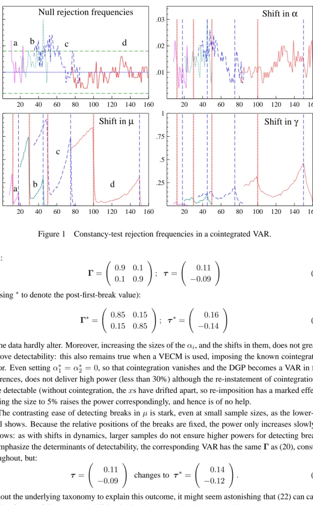
∆x2,t = γ2+α2(x1,t−1−x2,t−1−µ) +2,t (19) where_i,t∼IN[0, σ_ii], withE[_1,t2,s] = 0∀t, s. Four groups of experiments established the size of the test (when (19) is constant); the impacts of breaks inα₁andα₂; breaks in the long-run mean (µ₁); and breaks in the growth rates (γ1andγ2). Four sample sizes were considered: T = 24,60,100, and 200 (denoted a, b, c, d on graphs), with breaks at0.5T, reverting to the original parameter values at0.75T. Rejection frequencies at 1% nominal test sizes were recorded for 500 replications (standard errors of about 0.004). A known break point was assumed as this delivers the highest possible power for the test used – given that the aim is to check on low power – but results in the neighbourhood of the breaks are also shown. An unrestricted first-order VAR with intercept was estimated and tested.

The baseline experiment setα1 =−0.1andα2 = 0.1, both changed by+0.05(or5√σ11). Also,

µ = 1 (changed by +0.3, soα₁µchanged by3√σ₁₁). Settingβ0 = (1 :−1) enforcedγ₁ = γ₂, set equal to√σ_ii = 0.01 (roughly 4% p.a. growth for quarterly data, changed to0.02). The experiments are reported graphically, each panel showing all four sample-size outcomes for a given case; common random numbers were used to control inter-experiment variation. The start date of a break is shown by a vertical dotted line, and the end by a vertical dashed line: the design is such that all breaks end for a given sample size before the first one starts in the next larger sample.

As fig. 1 (first panel) reveals, the actual and nominal sizes are close: the approximate 95% confid-ence interval is (0.002, 0.018), shown on the graph as a dashed line. Few null rejection frequencies lie outside those bounds once the sample size exceeds 60, but there is some over-rejection at the smallest sample sizes, though never above 3%. These outcomes are not sufficiently discrepant to markedly affect the outcomes of the ‘power’ comparisons below.

The top-right panel demonstrates that a change in the coefficient of a zero-mean disequilibrium is not readily detectable: the powers are so low, do not increase with sample size, and barely reflect any breaks, that one might question whether the Monte Carlo was correctly implemented – be assured it was. This lack of detectability was predicted by the analysis above, by that in Clements and Hendry (1994), and was found in a different setting by Hendry and Doornik (1997), so is not likely to be spurious. This is despite the fact that both the dynamics and the intercepts shift considerably in the VAR representation:

20 40 60 80 100 120 140 160 .01

.02 .03

a

b

_c

d

Null rejection frequencies

20 40 60 80 100 120 140 160 .01 .02 .03

Shift in

α

a

b

c

d

Shift in

µ

Shift in

γ

Figure 1 Constancy-test rejection frequencies in a cointegrated VAR.

from: Γ= 0.9 0.1 0.1 0.9 ! ; τ = 0.11 −0.09 ! (20)

to (using∗to denote the post-first-break value):

Γ∗ ₌ 0.85 0.15 0.15 0.85 ! ; τ∗₌ 0.16 −0.14 ! (21)

yet the data hardly alter. Moreover, increasing the sizes of theα_i, and the shifts in them, does not greatly improve detectability: this also remains true when a VECM is used, imposing the known cointegrating vector. Even settingα∗₁ =α∗₂ = 0, so that cointegration vanishes and the DGP becomes a VAR in first differences, does not deliver high power (less than 30%) although the re-instatement of cointegration is more detectable (without cointegration, thexs have drifted apart, so re-imposition has a marked effect). Raising the size to 5% raises the power correspondingly, and hence is of no help.

The contrasting ease of detecting breaks inµis stark, even at small sample sizes, as the lower-left panel shows. Because the relative positions of the breaks are fixed, the power only increases slowly as

T grows: as with shifts in dynamics, larger samples do not ensure higher powers for detecting breaks. To emphasize the determinants of detectability, the corresponding VAR has the sameΓas (20), constant throughout, but: τ = 0.11 −0.09 ! changes to τ∗= 0.14 −0.12 ! . (22)

Without the underlying taxonomy to explain this outcome, it might seem astonishing that (22) can cause massive forecast failure, yet the shift in (21) is almost completely undetectable.

Finally, doubling the growth rate – a dramatic change in real growth – is again almost undetectable on these tests at smallT, but becomes increasingly easy to discern as the sample size grows: see the lower-right panel. Since the data exhibit a broken trend, but the model does not, larger samples with the same relative break-points induce effects of a larger magnitude. Thus, the type of structural break affects whether larger samples help. The model formulation also matters: if a VECM is used, the first growth break shows up much more strongly, as the shift inγ is isolated, whereas the VAR ‘bundles’ it withγ−αµ, where the second component can camouflage the shift (VAR estimates ofγ−αµhave large standard errors in anI(1) representation, whereas estimates ofγare usually precise). Even so, a large growth-rate change has a surprisingly small effect even atT = 200.

Hendry (1999) shows that pure changes in β toβ∗, whereE(β∗)0x_t−µ∗ = 0maintains the disequilibrium mean at zero, andβ0γ =0both before and after the shift, are also surprisingly hard to detect. In practice, the relevant shift inµwould be unknown, so an induced mean-shift would occur, making detection easy. Also, since the process drifts, power should rise quickly as the sample size grows.

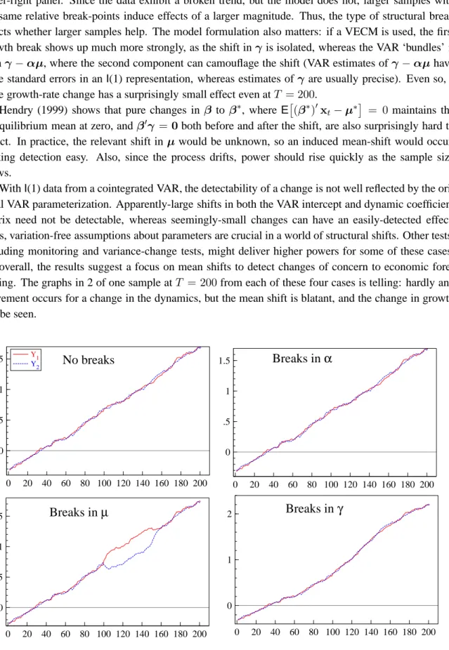
WithI(1) data from a cointegrated VAR, the detectability of a change is not well reflected by the ori-ginal VAR parameterization. Apparently-large shifts in both the VAR intercept and dynamic coefficient matrix need not be detectable, whereas seemingly-small changes can have an easily-detected effect. Thus, variation-free assumptions about parameters are crucial in a world of structural shifts. Other tests, including monitoring and variance-change tests, might deliver higher powers for some of these cases, but overall, the results suggest a focus on mean shifts to detect changes of concern to economic fore-casting. The graphs in 2 of one sample atT = 200from each of these four cases is telling: hardly any movement occurs for a change in the dynamics, but the mean shift is blatant, and the change in growth can be seen. 0 20 40 60 80 100 120 140 160 180 200 0 .5 1 1.5 Y1

_{No breaks}

Breaks in

µ

Breaks in

α

Breaks in

γ

7 Selecting models by forecast accuracy

A statistical forecasting system is one having no economic-theory basis, in contrast to econometric models for which economic theory is the hallmark.2 Since the former systems rarely have implications for economic-policy analysis – and may not even entail links between target variables and policy instru-ments – being the ‘best’ available forecasting device is insufficient to ensure its value for policy analysis. Consequently, the main issue is the converse: does the existence of a dominating forecasting procedure invalidate the use of an econometric model for policy? Since forecast failure often results from factors unrelated to the policy change in question, an econometric model may continue to characterize the re-sponses of the economy to a policy, despite its forecast inaccuracy. Further, when policy changes are implemented, forecasts from a statistical model may be improved by combining them with the predicted policy responses from an econometric model. Thus, forecasting models should remain distinct from policy models, as explained by Hendry and Mizon (1999).

The rationale for this analysis follows from the taxonomy of forecast errors in section 3 which re-corded that deterministic shifts were the primary source of systematic forecast failure in econometric models. Devices like intercept corrections can robustify forecasting models against breaks which have occurred prior to forecasting (see e.g., Clements and Hendry, 1996a, and Hendry and Clements, 1999). While such ‘tricks’ may mitigate forecast failure, the policy-analysis implications of the resulting mod-els are neither more nor less useful than those of the failed counterparts. Conversely, post-forecasting policy changes will induce breaks in models that did not embody the relevant policy links, whereas econometric systems need not experience that policy-regime shift. Consequently, when both structural breaks and regime shifts occur, neither class of model alone is adequate: this suggests that they should be combined, and Hendry and Mizon (1999) propose, and empirically illustrate, one approach to doing so.

8 Modelling shifts

Modelling and/or offsetting changes in deterministic terms is manifestly important. To allow for ex ante breaks needs foresight from some extra-model source (such as judgement, or early-warning signals). Unfortunately, we do not yet know how to predict when economic ‘meteors’ will strike, and can but advise on what to do after they have hit. Recurrence of shifts would allow models of their behavior, as in regime-shifting equations, though there are other possibilities, such as the approach in Engle and Smith (1998). Improved ntercept corrections may be possible: Clements and Hendry (1998c) and section 8.1 discuss some ideas.

Regime-shifting models, such as Markov-switching autoregressions, as in Hamilton (1989, 1993), or self-exciting threshold autoregressive models, as in Tong (1978), seek to model changes by including stochastic and deterministic shifts in their probability structure. By separately modelling expansionary and contractionary phases of business cycles, say, an implicit assumption is that the shifts are regular enough to be modelled. In practice, the forecasting superiority of such approaches is controversial: conditional on being in a particular regime, these models may yield gains (see, e.g., Tiao and Tsay, 1994, and Clements and Smith, 1999), but unconditionally there is often little improvement over linear models on criteria such asMSFE(see, e.g., Pesaran and Potter, 1997, and Clements and Krolzig, 1998). However, they may be favoured on qualitative measures of forecast performance, or by approaches that evaluate the whole forecast density (Clements and Smith, 2000). Given the prominence of deterministic

shifts as an explanation for forecast failure, efforts to model such shifts may yield significant rewards.

8.1 Intercept corrections

When the source of a model’s mis-specification is known, it is usually corrected, but in many set-tings, mis-specifications are unknown, so are difficult to correct. One widely-used tool is intercept correction (denoted IC), which sets the model ‘back on track’ to start from the actual forecast origin

x_T. Hendry and Clements (1994) develop a general theory of intercept corrections, and Clements and Hendry (1996b) show that such corrections can robustify forecasts against breaks that have happened, but only at the cost of an increase in forecast-error variance. The form of correction envisaged in that analysis is such that the correction alters as the forecast origin moves through the sample – the correc-tion is always based on the error(s) made at, or immediately prior to, the forecast origin. However, those forms of correction require a steadily-expanding information set, and can be implemented by adding an indicator variable equal to unity from the last sample observation onwards, so that the same correction is applied at all forecast origins. An IC will work if, immediately prior to forecasting, the model is mis-fitting by a substantial amount, so ‘shifting’ the forecast origin towards the data will offset much of the later mis-forecasting. To reduce the forecast-error variance, the IC can be set to unity for the last few sample observations.

Alternatively, ICs can be based on the comparative robustness of different forecasting models to breaks, using say the DDV forecasts to intercept correct an econometric model. Such an approach is close to that advocated by Hendry and Mizon (1999).

9 Implications for models of expectations formation

In an economy made non-stationary by unanticipated deterministic shifts, ‘rational expectations’ as-sumptions are stringent, since they require agents not only to know all the relevant information, but also to know how every component enters the joint data density at each point in time, when many of the events and their consequences cannot be easily unanticipated. ‘Rational agents’ would be unwise to use model-based expectations, when models – including their own – are manifestly mis-specified for a non-constant LDGP. These claims are clear from (6): the model error e_T+h|T equals the ‘rational expectations’ error ε_T+h|T if and only if every other term is zero.3 When bx_T+h|T =

ET+h[xT+h|X1T,{Q∗}1T+h], then indeed (6) collapses to leave only εT+h|T, but the required

impli-cit knowledge of recent and future deterministic and stochastic shifts is untenable. Moreover, once

{Q∗_}1

T+his replaced byQ1T+handET+h byET, previous sections showed that the resulting forecasts

can be dominated by methods that use no causally-relevant variables. ‘Sensible’ agents might learn that they cannot form expectations any better than such forecasting models, and so adopt ‘robust forecasting rules’. Since such ‘rule’ have the property that they do not usually vary with policy changes, although their forecasts do, they have interesting implications for the Lucas (1976) critique, discussed in the next section..

In practice, the claim by several non-nested macro-models to embody ‘rational expectations’ is contradictory: at most one could be correct, and at best the rest have ‘model consistent’ expectations. But since such models are bound to be mis-specified, ‘model consistent’ expectations have no formal basis in the processes considered here. Indeed, they seem to embody the worst of all possible features: they are not robust to structural change, unlike robust rules, and do not coincide with how agents actually form expectations.

9.1 Implications for the Lucas critique

Lucas (1976) criticized the use of estimated econometric models for policy analysis in the following quote:

“...Given that the structure of an econometric model consists of optimal decision rules for economic agents, and that optimal decision rules vary systematically with changes in the structure of series relevant to the decision maker, it follows that any change in policy will systematically alter the structure of econometric models...” Lucas [1976, p.41].

There are several questionable assumptions essential for Lucas’s assertion. First, that “optimal decision rules vary systematically with changes in the structure of series relevant to the decision maker” – unanticipated deterministic shifts are among the most drastic changes facing agents, yet the robust forecasting rules described above do not alter with them. Thus, an econometric model in which variables such as ∆x_t entered representing ∆ex_t|t−1 would not necessarily change even when forecast failure occurred (‘gear changes’ of the kind discussed by Flemming, 1976, shifting variables fromI(1) toI(2) say, could induce changed forecasting rules). In fact, this is precisely the formulation discussed by Favero and Hendry (1992), albeit on completely different grounds.

Secondly, “that any change in policy will systematically alter the structure of econometric models” conflates regime shifts in policy, when the underlying rules are altered, and different policy-variable values within the same regime. Provided the models embody the policy variables of relevance, changes in their values will be correctly reflected, and changes in rules need not alter them.

The third, less obvious, assumption, is that agents can extract the “structure of series relevant to the(m)”, and this seems untenable in precisely the type of processes consistent with intermittent forecast failure. Thus, the critique is far from being an explanation for forecast failure, and does not entail the implication that econometric models have no future in a world where policy rules change.

The final implicit assumption is that any changes in econometric models will have noticeable empir-ical consequences. As we have seen, zero-mean changes are difficult to detect, and do not necessarily disrupt forecasts. Thus, the unimportant consequences of such changes, rather than their absence, could account for the lack of empirical evidence that the critique occurs: see Ericsson and Irons (1995). Nev-ertheless, for policy models, such undetected changes could be hazardous: the estimated parameters would appear to be constant, yet be mixtures across regimes, leading to inappropriate advice – in partic-ular, Hendry (1999) shows that estimated impulse responses could have the wrong sign in VARs where breaks are not detectable. In the context of a progressive research (i.e., from the perspective of learning), this is unproblematic for econometric systems, since most policy changes involve deterministic shifts (as opposed to mean-preserving spreads), hence earlier incorrect inferences will be detected rapidly. Unfortunately, that is cold comfort to the policy maker, or the economic agents subjected to the wrong policies.

10 Conclusion

The generalized and VECM taxonomy of forecast errors shown above, and the resulting derivations of forecast-error biases and variances, suggest that deterministic shifts are a primary source of serious forecast failure. The taxonomies predicted that differencing several times would be effective, when breaks have occurred, for forecast evaluation over short horizons. The simulation results illustrated the relative difficulties of detecting breaks in deterministic and other parameters. In a four-variable empirical example of forecasting using a small monetary model of the UK, when there was a known major financial innovation, Clements and Hendry (1998b) show that the theoretical results match the

outcomes over both pre- and post-break forecast periods for the three methods considered above, and confirmed the effectiveness of the intercept-correction strategies they investigated. These findings are also consistent with the results of using a large macro-econometric system as reported in Eitrheim et al. (1997). Thus, although other forms of structural break, model mis-specification, a lack of parsimony including failing to impose restrictions such as unit roots and cointegration, inaccurate forecast-origin data, and inefficient estimation may all exacerbate forecast failure, we believe they play supporting roles, as found in Hendry and Doornik (1997).

One consequence of these results is to caution against automatic adoption of a method that happens to win a particular forecasting competition: careful analysis as to why is strongly recommended. If a deterministic shift is suspected, or confirmed, then methods that are not robust to such a shift are likely to have performed poorly. That would not necessarily preclude the continued use of a model that suffered forecast failure, subject to appropriate intercept corrections being used. In the policy context of forecasting after a structural break, where policy is then altered, Hendry and Mizon (1999) show the benefits of using a ‘time-series’ model (such as the DDV) to intercept correct the econometric system, when the latter is retained for policy analysis despite forecast failure.

Finally, the stringent requirements for forming ‘rational expectations’ were described, and the im-plications noted for the Lucas critique of agents’ adopting robust forecasting methods.

References

Allen, P. G., and Fildes, R. A. (1998). Econometric forecasting strategies and techniques. Mimeo, University of Massachussets, USA. Forthcoming, J. S. Armstrong, (ed.) Principles of Forecasting, Kluwer Academic Press.

Bontemps, C., and Mizon, G. E. (1996). Congruence and encompassing. Economics department, mimeo, European University Institute.

Calzolari, G. (1981). A note on the variance of ex post forecasts in econometric models. Econometrica,

49, 1593–1596.

Clements, M. P., and Hendry, D. F. (1994). Towards a theory of economic forecasting. In Hargreaves, C. (ed.), Non-stationary Time-series Analysis and Cointegration, pp. 9–52. Oxford: Oxford Uni-versity Press.

Clements, M. P., and Hendry, D. F. (1995). Forecasting in cointegrated systems. Journal of Applied

Econometrics, 10, 127–146.

Clements, M. P., and Hendry, D. F. (1996a). Intercept corrections and structural change. Journal of

Applied Econometrics, 11, 475–494.

Clements, M. P., and Hendry, D. F. (1996b). Intercept corrections and structural change. Journal of

Applied Econometrics, 11, 475–494.

Clements, M. P., and Hendry, D. F. (1998a). Forecasting Economic Time Series. Cambridge: Cambridge University Press. The Marshall Lectures on Economic Forecasting.

Clements, M. P., and Hendry, D. F. (1998b). On winning forecasting competitions in economics. Spanish

Economic Review, 1, 123–160.

Clements, M. P., and Hendry, D. F. (1998c). Using time-series models to correct econometric model forecasts. mimeo, Institute of Economics and Statistics, University of Oxford.

Clements, M. P., and Hendry, D. F. (1999a). Forecasting Non-stationary Economic Time Series: The

Clements, M. P., and Hendry, D. F. (1999b). On winning forecasting competitions in economics. Spanish

Economic Review, 1, 123–160.

Clements, M. P., and Krolzig, H.-M. (1998). A comparison of the forecast performance of Markov-switching and threshold autoregressive models of US GNP. Econometrics Journal, 1, C47–75. Clements, M. P., and Smith, J. (1999). A Monte Carlo study of the forecasting performance of empirical

SETAR models. Journal of Applied Econometrics, 14, 124–141.

Clements, M. P., and Smith, J. (2000). Evaluating the forecast densities of linear and non-linear models: Applications to output growth and unemployment. Journal of Forecasting. Forthcoming.

Doornik, J. A. (1996). Object-Oriented Matrix Programming using Ox. London: International Thomson Business Press and Oxford: http://www.nuff.ox.ac.uk/Users/Doornik/.

Doornik, J. A., and Hendry, D. F. (1998). Monte Carlo simulation using PcNaive for Windows. Unpub-lished typescript, Nuffield College, University of Oxford.

Eitrheim, Ø., Husebø, T. A., and Nymoen, R. (1997). Error-correction versus differencing in macroe-conometric forecasting. Mimeo, Department of Economics, University of Oslo.

Engle, R. F., and Smith, A. D. (1998). Stochastic permanent breaks. Discussion Paper No. 99-03, University of California, San Diego.

Ericsson, N. R., and Irons, J. S. (1995). The Lucas critique in practice: Theory without measurement. In Hoover, K. D. (ed.), Macroeconometrics: Developments, Tensions and Prospects. Dordrecht: Kluwer Academic Press.

Favero, C., and Hendry, D. F. (1992). Testing the Lucas critique: A review. Econometric Reviews, 11, 265–306.

Fildes, R. A. (1992). The evaluation of extrapolative forecasting methods. International Journal of

Forecasting, 8, 81–98.

Flemming, J. S. (1976). Inflation. Oxford: Oxford University Press.

Hamilton, J. D. (1989). A new approach to the economic analysis of nonstationary time series and the business cycle. Econometrica, 57, 357–384.

Hamilton, J. D. (1993). Estimation, inference, and forecasting of time series subject to changes in regime. In Maddala, G. S., Rao, C. R., and Vinod, H. D. (eds.), Handbook of Statistics, Vol. 11: Amsterdam: North–Holland.

Hendry, D. F. (1996). On the constancy of time-series econometric equations. Economic and Social

Review, 27, 401–422.

Hendry, D. F. (1997). The econometrics of macro-economic forecasting. Economic Journal, 107, 1330– 1357. Reprinted in T.C. Mills (ed.), Economic Forecasting. Edward Elgar, 1999.

Hendry, D. F. (1999). On detectable and non-detectable structural change. Mimeo, Nuffield College, University of Oxford.

Hendry, D. F., and Clements, M. P. (1994). On a theory of intercept corrections in macro-economic forecasting. In Holly, S. (ed.), Money, Inflation and Employment: Essays in Honour of James

Ball, pp. 160–182. Aldershot: Edward Elgar.

Hendry, D. F., and Clements, M. P. (1999). Economic forecasting in the face of structural breaks. In Holly, S., and Weale, M. (eds.), Econometric Modelling: Techniques and Applications. Cam-bridge: Cambridge University Press. Forthcoming.

Hendry, D. F., and Doornik, J. A. (1997). The implications for econometric modelling of forecast failure.

Hendry, D. F., and Mizon, G. E. (1999). On selecting policy analysis models by forecast accuracy. Festschrift in Honour of Michio Morishima, STICERD, London School of Economics.

Johansen, S., and Juselius, K. (1990). Maximum likelihood estimation and inference on cointegration – With application to the demand for money. Oxford Bulletin of Economics and Statistics, 52, 169–210.

Lucas, R. E. (1976). Econometric policy evaluation: A critique. In Brunner, K., and Meltzer, A. (eds.),

The Phillips Curve and Labor Markets, Vol. 1 of Carnegie-Rochester Conferences on Public Policy, pp. 19–46. Amsterdam: North-Holland Publishing Company.

Makridakis, S. e. a. (1982). The accuracy of extrapolation (time series) methods: Results of a forecasting competition. Journal of Forecasting, 1, 111–153.

Pesaran, M. H., and Potter, S. M. (1997). A floor and ceiling model of US Output. Journal of Economic

Dynamics and Control, 21, 661–695.

Tiao, G. C., and Tsay, R. S. (1994). Some advances in non-linear and adaptive modelling in time-series.

Journal of Forecasting, 13, 109–131.

Tong, H. (1978). On a threshold model. In Chen, C. H. (ed.), Pattern Recognition and Signal Processing, pp. 101–141. Amsterdam: Sijhoff and Noordoff.

Turner, D. S. (1990). The role of judgement in macroeconomic forecasting. Journal of Forecasting, 9, 315–345.