Air Force Institute of Technology
AFIT Scholar
Theses and Dissertations Student Graduate Works
12-26-2014
Characterizing and Managing Intrusion Detection
System (IDS) Alerts with
Multi-Server/Multi-Priority Queuing Theory
Christopher C. Olsen
Follow this and additional works at:https://scholar.afit.edu/etd
Part of theSystems Engineering Commons
This Thesis is brought to you for free and open access by the Student Graduate Works at AFIT Scholar. It has been accepted for inclusion in Theses and Dissertations by an authorized administrator of AFIT Scholar. For more information, please [email protected].
Recommended Citation
Olsen, Christopher C., "Characterizing and Managing Intrusion Detection System (IDS) Alerts with Multi-Server/Multi-Priority Queuing Theory" (2014).Theses and Dissertations. 9.
CHARACTERIZING AND MANAGING INTRUSION DETECTION SYSTEM (IDS) ALERTS WITH MULTI-SERVER/MULTI-PRIORITY QUEUING
THEORY THESIS DECEMBER 2014
Christopher C. Olsen, Captain, USAF AFIT-ENV-MS-14-D-24
DEPARTMENT OF THE AIR FORCE AIR UNIVERSITY
AIR FORCE INSTITUTE OF TECHNOLOGY
Wright-Patterson Air Force Base, Ohio DISTRIBUTION STATEMENT A.
The views expressed in this thesis are those of the author and do not reflect the official policy or position of the United States Air Force, Department of Defense, or the United States Government. This material is declared a work of the U.S. Government and is not subject to copyright protection in the United States.
AFIT-ENV-MS-14-D-24
CHARACTERIZING AND MANAGING INTRUSION DETECTION SYSTEM (IDS) ALERTS WITH MULTI-SERVER/MULTI-PRIORITY QUEUING
THEORY
THESIS
Presented to the Faculty
Department of Systems Engineering and Management Graduate School of Engineering and Management
Air Force Institute of Technology Air University
Air Education and Training Command In Partial Fulfillment of the Requirements for the Degree of Master of Science in Systems Engineering
Christopher C. Olsen, BS Captain, USAF
December 2014
DISTRIBUTION STATEMENT A.
AFIT-ENV-MS-14-D-24
CHARACTERIZING AND MANAGING INTRUSION DETECTION SYSTEM (IDS) ALERTS WITH MULTI-SERVER/MULTI-PRIORITY QUEUING
THEORY
Christopher C. Olsen, BS Captain, USAF
Approved:
_______//SIGNED//____________________ _08 Dec 2014_
John M. Colombi, Ph.D. (Chairman) Date
_______//SIGNED//____________________ _08 Dec 2014_
Lt Col Kyle F. Oyama, Ph.D. (Member) Date
_______//SIGNED//____________________ _08 Dec 2014_ David R. Jacques, Ph.D. (Member) Date
Abstract
The DoD sets forth an objective to “employ an active cyber defense capability to prevent intrusions onto DoD networks and systems.” Intrusion Detection Systems (IDS) are a critical part of network defense architectures, but their alerts can be difficult to manage. This research applies Queuing Theory to the management of IDS alerts, seeking to answer how analysts and priority schemes effect alert processing performance. To characterize the effect of these two variables on queue wait times, a MATLAB simulation was developed to allow parametric analysis under two scenarios. The first varies the number of analysts and the second varies the number of alert priority levels. Results indicate that two analysts bring about drastic improvements (a 41% decrease) in queue wait times (from 116.1 to 49.8 minutes) compared to a single analyst, due to the reduced potential for bottlenecks, with diminishing returns thereafter. In the second scenario, it was found that three priority levels are sufficient to realize the benefits of prioritization, and that a five level priority scheme did not result in shorter queue wait times for Priority 1 alerts. Queuing models offer an effective approach to make IDS resource decisions in keeping with DoD goals for Active Cyber Defense.
Acknowledgments
There are a variety of faculty and staff at AFIT who I should thank for offering me guidance and encouragement all along the way. The biggest thanks go undeniably to Dr. John Colombi, who took me in when I was late into my thesis hours and added a significant amount of vector to my all-thrust approach. I’d also like to thank Dr. Kenneth Hopkinson from the Department of Electrical and Computer Engineering for helping me in my first, albeit overly ambitious, attempt at a thesis topic. Lt Col Kyle Oyama, as my final professor before beginning my thesis hours, provided a lot of advice and insight into how to select and begin writing a thesis topic. Many thanks to Capt Christina Rusnock for helping to kick start my thesis work, by showing me how to navigate the web of research databases in an organized way. I’d also like to extend much appreciation to Ms. Hallie Owsiany, the distance learning coordinator, for being so awesome the last few years at everything from registration to answering my oddball questions, many of which I’m sure were firmly outside her job description.
I’d be remiss not to thank my parents and grandparents for starting me out in life with the right attitude about and aspirations for higher education. Good grades and advanced degrees were never a discussion of “if” but always of “when” and “why”, and for that I can never thank them enough.
And of course, I have to thank my wife (a soon-to-be M.D.!) for letting me work through weekend after weekend when she (and let’s be honest, me too) would have rather been doing something a little more…fun.
Table of Contents
Page
Abstract ...v
Acknowledgments... vii
Table of Contents ... viii
List of Figures ...x
List of Tables ... xii
I. Introduction ...1 Background...1 Problem Statement...4 Research Focus ...4 Investigative Questions ...5 Methodology Overview ...5 Hypothesis ...5 Assumptions/Limitations ...6 Implications ...6 Organization of Thesis ...7
II. Literature Review ...8
Chapter Overview ...8
Current Techniques for IDS Alert Management ...8
Queuing Theory Primer ...10
Little’s Law and Queuing Theory Analytical Equations ...14
Foundations from Similar Research ...16
Summary...18
III. Methodology ...19
Chapter Overview ...19
Overview of Research Methodology ...19
Description of Dependent and Independent Variables ...19
Description of Analysis ...21
Construction of Model ...21
Validation of Model ...23
Assumptions ...33
Summary...34
IV. Analysis and Results ...35
Chapter Overview ...35
Scenario 1: Varying the Number of Analysts...35
Scenario 2: Varying the Number of Priority Levels ...44
Summary...50
V. Conclusions and Recommendations ...52
Summary of Research...52
Study Limitations ...53
Recommendations for Action ...53
Recommendations for Future Research...54
Significance of Research ...56
Appendix A ...57
MATLAB Model Code ...57
Bibliography ...69
List of Figures
Page Figure 1. An example IDS rule or “signature”. Each word sets the value for a
configurable parameter, determined by the rule format. This particular format is from the popular open source IDS called SNORT®. (Roesch & Green, 2014) ... 3 Figure 2. A basic queuing theory diagram calling out the six defining characteristics of a
system (Reed, 1995). ... 12 Figure 3. Comparison of the mean response time, or system transit time W, for multiple
servers fed by multiple queues (shown in red) versus multiple servers fed by a single queue (shown in green) (Reed, 1995). ... 17 Figure 4. Class diagram depicting how the Main Script of the model orchestrates between
the three classes to create a functioning queuing system. ... 23 Figure 5. Clockwise, the average Queue Size, System Size, System Wait Time, and
Queue Wait Time output by the model for a simple M/M/1 system (λ=10, μ=12). .. 25 Figure 6. For an M/M/3 system with λ=3 and μ=6, the model agrees with analytical
predictions of the four response variables. ... 28 Figure 7. Model output for the four response variables for an M/M/1 with 2 Priority
system. Red reference lines represent values predicted by analytical equations. ... 32 Figure 8. System response in terms of Wq, Lq, W, and L with an increasing number of
analysts under three different traffic loads. ... 38 Figure 9. The four response variables (Wq, W, Lq, and L) for Priority 3 (low) alerts under
Figure 10. The four response variables (Wq, W, Lq, and L) for Priority 2 (mid) alerts under Scenario 1 conditions. ... 42 Figure 11. The four response variables (Wq, W, Lq, and L) for Priority 1 (high) alerts
under Scenario 1 conditions. ... 43 Figure 12. The system-wide response variables for the nine cases in Scenario 2. ... 46 Figure 13. Response variables for the 3-priority case, broken out by individual priority
level across three traffic conditions. ... 47 Figure 14. Response variables for the 5-priority case, broken out by individual priority
List of Tables
Page Table 1. Governing equations for M/M/1, M/M/c, and M/M/1 with k-Priority queuing . 16 Table 2. Comparison of the average system dependent variable values output by the
model compared to theoretical predictions, for an M/M/1 system with λ=10 and μ=12. ... 26 Table 3. Comparison of the average system dependent variable values output by the
model compared to theoretical predictions, for an M/M/3 system with λ=3 and μ=6. ... 29 Table 4. Comparison of the model and theoretical dependent variable average values,
both overall and for each priority level, in an M/M/1 with 2 priority level system. .. 33 Table 5. Summary of the model parameters used to generate each of the nine cases in
Scenario 1. ... 37 Table 6. Summary of the model parameters used to generate each of the nine cases in
AFIT-ENV-MS-14-D-24
CHARACTERIZING AND MANAGING INTRUSION DETECTION SYSTEM ALERTS WITH QUEUING THEORY
I. Introduction
Background
Active Cyber Defense
In the Department of Defense Strategy for Operating in Cyberspace (DSOC), signed in July 2011 by Secretary Robert Gates, the DoD sets forth five strategic initiatives aimed at bringing U.S. cyber defense capabilities to a level that reflects the nation’s reliance on cyberspace. Strategic Initiative 2 states that the, “DoD will employ new defense operating concepts to protect DoD networks and systems.” Two objectives under this initiative are to “employ an active cyber defense capability to prevent
intrusions onto DoD networks and systems” and to develop “new defense operating concepts and computing architectures” (Dept of Defense Chief Information Officer, 2010).
The DSOC describes active cyber defense, or ACD, as a “synchronized, real-time capability to discover, detect, analyze, and mitigate threats and vulnerabilities”. The key idea behind ACD is that threat mitigation happens in cyber-relevant time. Cyber-relevant is an intentionally ambiguous descriptor whose value varies depending on the battlespace being discussed. It could be on the order of nanoseconds in the case of a CPU or seconds in the case of end-to-end SATCOM links.
The DSOC also refers to the development of new defense operating concepts in cyberspace. While the context of this statement refers to exploration of mobile media and cloud computing technology, this thesis will characterize the queuing of alerts generated by network intrusion detection systems and use this data to make recommendations about network operation center response options.
Intrusion Detection Systems
Intrusion detection systems (IDS) cover a wide variety of capabilities and implementations. An IDS can be used to detect any kind of undesirable traffic on a network. An IDS provides the same kind of intrusion detection for a computer network as a burglar alarm provides for a house. Traditionally, IDS come in two flavors: network-based IDS (NIDS) and host-network-based IDS (HIDS). NIDS are placed at a network gateway or along choke points in the network topology to sift through network traffic at large and identify traffic that is malicious, against network policy, or has other undesirable
characteristics. HIDS are located at specific network nodes to provide specialized traffic monitoring (Blackwell, 2004). When located at a PC, a HIDS might track central
processing unit (CPU) activity or random access memory (RAM) consumption to identify anomalous behavior. A HIDS could also be located at a node providing a specific
network service, such as a file transfer protocol (FTP) server or an e-mail server. When employed together, NIDS and HIDS can provide a powerful capability to detect
undesirable activity on a computer network.
In simple terms, an IDS works by examining packets as they come across the network and comparing them to a bank of signatures stored within the device. A
signature is a specially formatted block of text that tells the IDS what to look for in each packet it inspects. If a packet matches the criteria contained within the signature, the device performs a preprogrammed action against the packet, such as dropping the packet or flagging it for tracking purposes. The IDS usually generates an alert in a human-readable format for the administrator. The management of these alerts is the major topic of this thesis.
Figure 1. An example IDS rule or “signature”. Each word sets the value for a configurable parameter, determined by the rule format. This particular format is from the popular open source IDS called SNORT®. (Roesch & Green, 2014)
The set of signatures within an IDS is called its rule-set. While there are
numerous open and proprietary sources for rule-sets that will provide protection from an array of common and uncommon threats, the adoption of a rule-set must be done with care. Each network administrator must carefully craft a rule-set that is specialized for their network. Unlike antivirus definitions where a growing database is of little concern due to the discrete and slow arrival times of new files, IDS rule-sets can quickly become so large that they are no longer functional. The first issue is one of processing speed and bandwidth. As each packet enters the IDS it must be compared to every signature in the rule-set in real-time. For example, an in-line IDS residing on a 10 Gbps network could receive anywhere from 800,000 to 15,000,000 packets per second at maximum
bandwidth consumption (Schudel). Therefore, the presence of unnecessary rules can quickly overwhelm the IDS processors and create a network logjam. The second issue is that rule-sets that are not focused enough will generate too many alerts and/or false positives. It is the goal of the network administrator to craft a rule-set that permits the free flow of legitimate network traffic and minimizes false positives, while still correctly identifying all malicious or undesirable traffic.
Problem Statement
The numerous types and volume of alerts generated by network IDS drive the need for a disciplined approach in characterizing the flow of alerts to the network administrators dashboard, so that they can be effectively triaged, analyzed, and used to implement defensive actions to keep the network safe and operational.
Research Focus
The focus of this research is to characterize the flow of alerts generated by any number of IDS devices within a network. The specific device that an alert stems from is irrelevant from the analyst perspective. All the data needed to properly respond to the alert is contained within the alert message itself. Therefore, all alerts generated across all IDS residing on the network can flow into a single queue, from which network analysts pull alerts. This is a different approach to today’s common practice, which is for alerts to be dumped periodically into a log file, which may not be examined by an administrator or analyst for hours or days.
Understanding the nature of alert flows allows network administrators to make decisions about how many analysts to employ within a network operations center and how alerts should be prioritized in order to ensure alerts are analyzed while they are still relevant to the defense of the network.
Investigative Questions
The key variables associated with alert queuing are the number of analysts servicing alerts, how often alerts arrive into the queue, how long each analyst takes to service an alert, and how many priority levels will be assigned to alerts when configuring the IDS rule-set.
The core investigative question addressed in this thesis is, given varying amounts of traffic density, how does the queuing system performance respond to varying numbers of analysts and priority levels?
Methodology Overview
The methodology used in this thesis is a quantitative stochastic simulation and sensitivity analysis using a validated MATLAB model based in Queuing Theory. This simulation will be used to characterize system performance and generate data for making decisions about network operations and resourcing.
Hypothesis
The addition of more analysts, regardless of the other system variables, will most certainly result in reduced waiting time for alerts. Obviously, however, unlimited
resourcing is not practical. So the real question will be, are the system performance gains from the addition of analysts worth the additional resource investment?
When it comes to the number of priority levels, it is expected that giving all alerts equal priority will not lead to ideal system performance, as there are some rare signatures that may trigger catastrophic events. These should always be dealt with first, which is not feasible in a no-priority system. At the other extreme, too many priority levels may add unnecessary complexity with little to gain in terms of performance.
Assumptions/Limitations
As with all models, it is never possible to completely replicate real world conditions. Therefore, care must be taken to try and distill from the infinite pool of variables only those factors that are most important to the phenomenon at hand. More detailed assumptions relating to the specific queuing theory model of this thesis are listed in Chapter III. Predominately, the conclusions are limited by a lack of empirical data regarding arrival rate and service rate distributions for IDS alerts.
Implications
As the DoD transitions toward a posture of Active Cyber Defense, the
incorporation of more active network sensors that deliver real-time status updates and alerts to network operators is likely to grow. As these devices become more prolific across the network, the burgeoning data flow could easily overload administrators.
This work attempts to address part of that problem by characterizing the flow of alerts from IDS devices and managing the associated variables such that network operators can take timely action in defense of the DoD and Air Force network.
Organization of Thesis
The remainder of this paper is organized as follows. Chapter 2, Literature Review, discusses common methods of analyzing IDS alerts today, lays out the basic concepts and terminology of Queuing Theory, introduces Little’s Law and the analytical equations used in Chapter 3, and discusses some foundations from similar research. Chapter 3, Methodology, describes the research method applied and validates the queuing theory model by comparing sample simulation results to their analytical counterparts. Chapter 4, Analysis and Results, describes two different scenarios and interprets the modeling results in the context of network operations. Chapter 5, Conclusions and Recommendations, summarizes the research results, discusses limitations of the research and potential avenues for future work, and makes recommendations about applying the work to Department of Defense active cyber defense objectives.
II. Literature Review
Chapter Overview
The purpose of this chapter is to review current handling methods and research for network IDS, foundational theory and common practices that will be used to support the investigative questions and methodology in this thesis, and to discuss the useful findings of similar research efforts that this paper will reference or incorporate.
Current Techniques for IDS Alert Management
While IDS are widely used in a variety of networks, there are still common problems administrators face in deploying them effectively. The major problems include:
• Alert Flooding – unusually high traffic volume or poorly written rule-sets (which generate excessive false positives) can lead to extremely high volumes of IDS alerts. For large networks, hundreds of thousands of alerts per day can fill up administrator logs (Meyer). Additionally, known network attack vectors exist that allows malicious actors to carry out what is effectively a denial of service attack against IDS systems by flooding logs with useless alerts (Tedesco & Aickelin)
• Limited Scope of Information – IDS generate alerts from packet-level data. Therefore, they may not have enough information to report on complex protocol communications or shed light on malicious network activity that spans protocols or networking devices (Blackwell, 2004)
• False Negatives – even when signatures are written with due diligence, it is impossible for a network administrator to foresee every possible attack vector or weakness in a network, especially those that could stem from well-resourced or creative adversaries. This can create gaps of “false negatives” in the IDS, where malicious traffic passes through undetected because no signature exists to compare it against. (Meyer, 2008)
• Problems with Anomaly-Type Signatures - anomaly signatures are useful because they do not survey individual packets, but instead look at broad trends in network activity across a variety of ports and protocols to determine if something is occurring that is out of the ordinary. However, these signatures depend on having pristine real-world network data from which to create a normalized base to compare against. The problem with using real-world data is one can never be
certain that the data being used to establish the base is not itself contaminated with attacks.
The bulk of research efforts pertaining to IDS and alert management have focused on addressing the problems listed above, improving the ability of IDS to correctly detect malicious traffic, and to reduce the number of alerts produced by the devices to a
manageable volume. A sampling of the techniques developed to address these issues is shown below:
• Alert Correlation and Abstraction – alert correlation and abstraction is
succinctly defined as a “multi-step process that receives alerts from one or more intrusion detection systems as input and produces a high-level description of the malicious activity on the network” (Aziz, 2006). In other words, alerts are compared and lumped into related groups, then compiled into a more human-friendly format for presentation to the user. (Valeur, Vigna, Kruegel, & Kemmerer, 2004)
• Parsing Programs – some research has implemented the use of scripts that search the fields of an archive of alerts to delete duplicates and/or alerts with field values that are likely to be false positives (Meyer, 2008). The result is a list of alerts that are more likely to contain alerts that contain information about truly threatening traffic.
• Alert Correlation with Known Network Vulnerabilities – investigations have been made into cross-referencing IDS alerts with a database of known network vulnerabilities, to increase the confidence that alerts presented to administrators contain relevant information. (Raulerson, Hopkinson, & Laviers, 2014) (Morin, Me, Debar, & Ducasse)
Once the volume of alerts have been reduced by techniques like those described above, they are usually dumped into a log file (Meyer, 2008). The administrator or network analysts can then go back and review the log file. This approach has the
advantage of allowing an analyst with a trained eye to survey a large number of historical alerts in search of unusual patterns. However, the main problem is that this analysis is not conducted in real-time, and does not meet the intent of an “active” cyber defense.
While useful for reviewing network activity over a large chunk of operating time (an entire day or weeks’ worth of activity), it is not appropriate for protecting the network in real-time, especially while an attack is underway or during a time of heightened defense posture. Since the status of a network can change very quickly, it may be too late if an analyst receives an alert even more than a few minutes after it is generated. For these times, what is needed is a disciplined way of triaging alerts and presenting them to network analysts so they can be assessed while they are still relevant to the defense of the network. In pursuit of a method to do just that, Queuing Theory is discussed in the following section as a potential solution.
Queuing Theory Primer
Practical Uses
Queuing Theory is the mathematical study of waiting in lines. The primary goals of queuing theory models are to determine the expected length of a line, or queue, and the average amount of time a customer can expect to spend in the system. The term "system" refers to the collective sum of those objects waiting in the queue plus those currently being served. To give a commonplace example, consider the customer experience at a supermarket checkout counter. The customers enter the store, select items for purchase, and then proceed to the checkout area. Upon arrival, the customers selects an available register and stands in line. Each customer can expect to wait in line for some average amount of time before reaching the cashier. Once at the cashier, the customer will again wait some amount of time while items are scanned and payment is taken. When payment is received, the customer exits the store with their goods and the process is complete.
Other applications for queuing theory include:
• Bank teller service lines (Cogdill & Monticino, 2007)
• Telecommunications traffic (Rasch, 1963)
• Traffic intersections
• Telephone customer service centers
• CPU task assignment
• Amusement park rides
Clearly, queuing theory can be a valuable tool for reducing wait times and increasing throughput in a variety of systems. The implications for reduced waste,
increased profit, customer satisfaction, and general system improvement continue to drive research into increasingly complex areas of queuing theory and queuing networks.
In the context of the IDS alert management problem, queuing theory offers an excellent framework for building an executable model to demonstrate the generation, flow, and handling of IDS alerts within a network.
Queuing System Characteristics
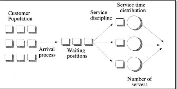
A queuing system is defined by six independent, or characterizing, variables:
• A source or population – consists of all potential objects (customers, tasks, etc.)
• An arrival process or distribution – how frequently objects enter the queue
• A queue or queues – where objects wait to be assigned to a server
• One or more servers – the person or machine that services objects
• A service time distribution – how long a server takes to do its task
• A service discipline – an algorithm dictating how objects are pulled from the queue
Figure 2. A basic queuing theory diagram calling out the six defining characteristics of a system (Reed, 1995).
The popular Kendall Notation is often used to quickly describe the characteristics of a given queuing system. A generalized Kendall Notation is of the form,
A/S/m/B/K/SD where,
A is the arrival distribution, S is the service time distribution, m is the number of servers,
B is the number of “buffer” spaces or the capacity of the queuing area, K is the population size, and
SD is the service discipline in use.
Many times, only the first three positions of Kendall Notation are used. In these cases, it can be assumed the buffer capacity and population are infinite and the service discipline is First Come, First Served (FCFS) or First In, First Out (FIFO). A common
simple model is M/M/1, where M denotes memoryless (i.e. Markovian) distributions, such as exponential, for inter-arrival and service times, and the system has 1 server.
There are numerous types of distributions, queue/server setups, and service disciplines that can be used to define a queuing system. The variables of particular interest in this paper are the arrival distribution, service distribution, number of servers, and the service discipline.
Once a system is characterized, the values of four dependent variables can be determined:
• L = Total number of objects in the system
o Lq = Number of objects waiting in the queue(s)
o Ls = Number of objects receiving service
• W = Amount of time an object spends in the system o Wq = Time spent waiting in the queue
o Ws = Time spent receiving service
Data concerning jobs in the system can provide information about system capacity and whether the system is overcrowded or underutilized. Similarly, data regarding wait times and service times can be useful metrics for determining system efficiency and identifying process bottlenecks.
It is possible, for simple queuing systems, to analytically develop a set of
governing equations which determine the values for the dependent variables listed above. These equations will be introduced in the next section and demonstrated in Chapter III to prove the accuracy and calibration of the alert queuing model under simple conditions. For the alert management problem explored in Chapter IV, however, complexity makes the development of analytical solutions infeasible. Therefore, a model provides a
mechanism to gather empirical data and provide insight beyond the reach of analytical closed-form solutions.
Little’s Law and Queuing Theory Analytical Equations
A foundational law for solving queuing problems analytically is Little’s Law, first proved by John D.C. Little in 1961. It states,
The time average number of customers in a queuing system, L, is equal to the rate at which customers arrive and enter the system, λ, times the average sojourn time of a customer, W (Sigman)
Or simply,
𝐿=𝜆𝑊
Using Little’s law as a foundation, governing equations can be derived for many simple queuing systems. Table 1 shows the governing equations for M/M/1, M/M/c, and M/M/1 with k-Priority queuing systems.
For an M/M/c system where multiple servers are utilized, another variable is introduced, ρ0,0, which is the probability that at any given time there are zero alerts
waiting in the queue and zero busy analysts. This value is used in computing the average length of the queue, Lq, from which the other variables are determined easily using Little’s Law.
When a First Come, First Served service discipline with priority is introduced (M/M/1 w/k-Priority in Table 1) it is necessary to calculate 𝑅�, the mean residual service time in the system. Alerts of lesser priority will have to wait for all alerts of higher priority to clear the system before being serviced. The mean residual service time is the sum of this extra waiting time for lower classes introduced by the prioritized service
discipline. Once 𝑅� is calculated, the simplest approach is the calculate how long alerts of each priority will wait in the queue, 𝑊𝑞𝐾. Determining the values of the other variables is then straightforward.
It was once thought that analytically determining the dependent variables for an M/M/c w/k-Priority system was not feasible, because mean residual service times would become too difficult to determine if each k priority level had a different mean service time (Virtamo). However, a 2005 paper by Harchol-Balter et al introduced Recursive Dimensionality Reduction (RDR) as an analytical approach to analyze multi-server queuing systems with multiple priority classes (Harchol-Balter, Osogami, Scheller-Wolf, & Wierman, 2005) RDR was shown to be accurate to modeling within 2%. However, the effectiveness of RDR was reduced with increasing numbers of servers and priority levels. Thus, the value of a dynamic queuing model that can handle varying service time
parameters for differing numbers of servers and priority levels becomes apparent, since it is possible to yield results that can be too complex for analytical investigation.
Table 1. Governing equations for M/M/1, M/M/c, and M/M/1 with k-Priority queuing Variable M/M/1 M/M/c M/M/1 w/k-Priority L =𝜆𝑊 = 𝐿𝑞+𝜆 𝜇 𝐿=𝐿𝑞+𝜆𝜇1+⋯+𝜆𝜇𝑘 𝐿𝑘 =𝐿 𝑞 𝑘+𝜆𝑘 𝜇 Lq = 𝜆𝑊𝑞 =�𝜌0,0� ⎣ ⎢ ⎢ ⎡ �𝜆𝜇�𝑐+1 (𝑐 −1)!�𝐶 − 𝜆𝜇�2⎦⎥ ⎥ ⎤ 𝐿𝑞 =𝐿 𝑞 1 +⋯+𝐿 𝑞 𝑘 𝐿𝑞𝑘 =𝜆 𝑘𝑊𝑞𝑘 W = 1 𝜇 − 𝜆 = 𝐿 𝜆 𝑊 = 𝜆1𝑊𝜆1 +⋯+𝜆𝑘𝑊𝑘 1+⋯+𝜆𝑘 𝑊𝐾 =𝑊𝑞𝑘+1𝜇 Wq =𝑊 −1 𝜇 = 𝐿𝑞𝜆 𝑊𝑞= 𝜆1𝑊𝑞 1 +⋯+𝜆 𝑘𝑊𝑞𝑘 𝜆1+⋯+𝜆𝑘 𝑊𝑞𝐾=(1− 𝜌1− ⋯ − 𝜌𝑘−1𝑅�)(1− 𝜌1− ⋯ − 𝜌𝑘) 𝜌0,0 --- = 1 �𝜆𝜇�𝑐�𝑐1!� �1− 𝜌�1 +∑𝑟=𝑐−1�𝜆𝜇�𝑟�𝑟1!� 𝑟=0 --- 𝑅� --- --- =1 2� 𝜆𝑘𝑆���𝑘2 𝑘 𝑘=1 𝑆𝑘2 ��� --- --- = 𝑛! 𝜇2
Foundations from Similar Research
Single Queue, Multiple Servers
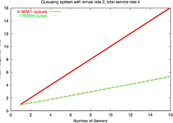
The queuing model used in this research relies on the premise that a single queue feeding multiple servers operates more efficiently (i.e. with reduced sojourn time through the system and thus less wait time in the queue) than multiple servers each fed by their own queue.
Figure 3, adapted from a publicly available lecture from University of Illinois (Reed, 1995), compares the mean response time, or system transit time W, of multiple servers each fed by their own queue (m M/M/1 queues shown in red) versus that of multiple servers fed by a single queue (1 M/M/m, or 1 M/M/c, queue shown in green). For all server quantities greater than one, a single M/M/c queue shows improved performance over multiple M/M/1 queues. At ten servers, the M/M/c queue processes objects through the queue approximately 70% faster than multiple M/M/1 queues.
Figure 3. Comparison of the mean response time, or system transit time W, for multiple servers fed by multiple queues (shown in red) versus multiple servers fed by a single queue (shown in green) (Reed, 1995).
Summary
This chapter presented the current techniques for IDS alert management and the research being conducted to improve these systems. It also discussed the basics of Queuing Theory, which is a simple but powerful tool that can be applied to a variety of situations where objects or tasks must wait to be serviced. The analytical mathematics can become difficult with increasing model complexity, but can be calculated for simple systems to a sufficient level for cross-checking results from computer simulations. The queuing model written for this research relies on the principal that a single queue feeding multiple servers is more efficient than multiple servers, each with its own queue. The next section will discuss the methodology for this research and demonstrate the validity of the MATLAB model.
III. Methodology
Chapter Overview
The purpose of this chapter is to describe the research approach and modeling procedures. First a brief overview of the methodology will be conducted, followed by a discussion of the relevant variables. Next, the custom queue model used will be
described and then data collected from the model will be compared against theoretical values to prove model accuracy and calibration. Finally, significant underlying assumptions to the experimental process will be discussed.
Overview of Research Methodology
The methodology employed was a computer based simulation model written by the author within the MATLAB computing environment (version R2013a). Since the primary objective of the research was to characterize Alert queuing for Intrusion
Detection Systems, the model was founded in Queuing Theory principles as presented in the Queuing Theory primer in Chapter II. This led to the creation of a flexible model which was used to generate data for parametric analysis in determining the sensitivity of the system to changes in the relevant Queuing Theory variables.
Description of Dependent and Independent Variables
In order to provide flexibility, the model allows for several user-defined variables. The duration of the simulation is determined by the number of arrivals of the lowest level priority alert, which the user defines. The model will continue to run until that number of arrivals is reached.
Users must also define other key Queuing Theory parameters including the number servers (Analysts in this case), the number of Alert priority levels, the inter-arrival rate for each priority level (1/λ), and the service time parameter for each priority level (1/μ). In the version used in this paper, inter-arrival and service time distributions are limited to the exponential form.
Experimental Design
This research uses a “validate and extend” approach to ensure the modeling results on which analysis is conducted are reliable. The first step was to run the simulation under conditions that were easily calculated with the analytical closed-form equations introduced in Chapter 2. The computer-based modeling results were then compared to these analytical equations to ensure the program was producing accurate results. The results of these calibration runs are presented later in this chapter.
Once the model was validated, the parameter values were extended beyond the reach of analytical equations, to generate empirical data for parametric analysis. The analysis was used to characterize the effect of dependent variables on overall system performance and finally to draw practical conclusions about applications to network operations.
Experimental Tasks
1) Design and write a MATLAB model. 2) Develop the set of analytical equations. 3) Validate the MATLAB model.
5) Run Scenario 1.
6) Analyze the results from Scenario 1
7) Make parameter assumptions for Scenario 2. 8) Run Scenario 2.
9) Analyze the results from Scenario 2.
Description of Analysis
Analysis was divided into two phases. The first phase compared model output under simple conditions to results predicted by analytical equations. This demonstrated the model was accurate and calibrated. This step was necessary to provide assurance that future data output based on more complex conditions, which cannot be checked
analytically, was reliable.
The second phase runs the model under more complex, realistic conditions. The model is run with careful variation in parameters to generate 3D surface plots that
demonstrate the sensitivity of the system. The second phase of analysis was divided into two Scenarios that will be discussed in Chapter 4.
Construction of Model
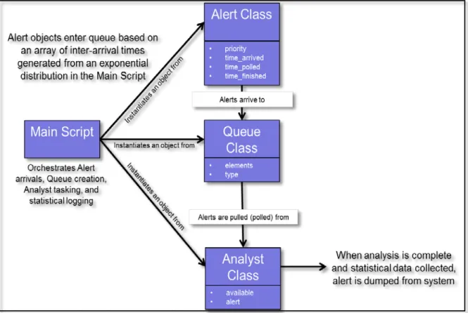
The complete MATLAB code for the model used in this research is included in the Appendix, but a brief description of how the model works is provided. The model uses object-oriented programming techniques to generate a functioning queue and set of servers (or analysts). A main script orchestrates alert arrivals, queue management, analyst tasking, and metric/statistical logging. The main script allows the user to define the total number of alert arrivals (which equates to the length of the simulation), the
number of analysts, the number of priority levels, and to define an arrival rate and service rate for each priority level.
An alert class is used to construct alert objects, each of which has 4 properties associated with it: the alert priority level (priority), the time it arrived into the queue (time_arrived), the time it was polled (or pulled) from the queue (time_polled), and the time it reached service completion and exited the system (time_finished).
A queue class is used to construct the queue object(s). Queue objects have properties for type, which is always of type alert objects in this research, and individual elements, which are the queue locations that each alert is placed into.
Finally, there is an analyst class, which creates analyst objects that have a Boolean property of being available or busy (available) and an alert property, which is where they store the current alert they are servicing.
Figure 4 is a class diagram to show how the various classes interact with the main script to produce a complete queuing theory model.
Figure 4. Class diagram depicting how the Main Script of the model orchestrates between the three classes to create a functioning queuing system.
Validation of Model
For assurance that the model generates reliable and accurate data, model output was compared with Queuing Theory analytical results for a set of simple parameters.
Before proceeding, recall from Chapter I that Kendall notation of the form A/S/m/B/K/SD is the standardized method of describing queuing systems. Many times, only the first three positions of Kendall Notation are used. In these cases, it can be assumed the buffer capacity and population are infinite and the service discipline is First Come, First Served (FCFS). Thus, M/M/1 = M/M/1/∞/∞/FCFS.
M/M/1Analytical Results
Perhaps the simplest Queuing Theory system is the M/M/1, where M represents an exponential distribution. Therefore, in an M/M/1 system Alert inter-arrivals and service times are based on an exponential distribution and there is only one server, or Analyst.
For comparison to model results, assume an arrival rate of λ = 10 alerts per hour (1/λ = 1/10, or an alert arrives on average every 6 minutes) and a service rate of µ=12 alerts per hour (1/μ = 1/12, or one alert is serviced on average every 5 minutes).
Therefore, the average time each alert spends in the system (sitting in the queue plus the time it takes to be serviced), W, is
𝑾=µ− 𝝀𝟏 =𝟏𝟐 − 𝟏𝟎𝟏 =𝟏𝟐 𝒐𝒓 .𝟓𝒉𝒐𝒖𝒓𝒔 (𝟑𝟎𝒎𝒊𝒏𝒔)
the average time each alert sits in the queue before getting serviced, Wq, is
𝑾𝒒=𝑾 −𝟏µ= 𝟏𝟐−𝟏𝟐𝟏 =𝟏𝟐𝟓 𝒐𝒓 .𝟒𝟏𝟕𝒉𝒐𝒖𝒓𝒔 (25 mins)
the average number of alerts in the system, L, is
𝑳= 𝝀𝑾= (𝟏𝟎)�𝟏𝟐�=𝟏𝟎𝟐 =𝟓𝒂𝒍𝒆𝒓𝒕𝒔
and the average number of alerts in the queue, Lq, is
𝑳𝒒= 𝝀𝑾𝒒= (𝟏𝟎)�𝟏𝟐�𝟓 =𝟓𝟎𝟏𝟐=𝟒.𝟏𝟔𝟕𝒂𝒍𝒆𝒓𝒕𝒔
M/M/1 Model Results
The data in Figure 5 shows convergence to theoretical values over a trial run of 100,000 alert arrivals using the same values of λ=10 and µ=12. The red reference lines represent the theoretical values.
It should be noted queue size, Lq, and system size, L, throughout this analysis are based on a sampling of simulation time, anywhere from every 1,000 to 10,000 minutes depending on the complexity and total simulation time of the model. Due to the varying arrival rates and priority levels in use, simulation time could expand to millions of time steps, with a separate array required for each priority level. Continuous evaluation of the average queue and system size for every iteration of simulation time proved to be too computationally intense for the home PC to handle.
Figure 5. Clockwise, the average Queue Size, System Size, System Wait Time, and Queue Wait Time output by the model for a simple M/M/1 system (λ=10, μ=12).
At steady state, the model converges to the theoretical reference lines pictured. There is, however, a transient period where the average size and wait time values fluctuate drastically. In order to negate the effects of the transient period when calculating model error, only the last 10% of the curve data points are used when calculating root-mean-squared (RMS) error.
The average values of the response variables as predicted by the model are compared to the theoretical values in Table 2. The small RMS errors suggest the model is an excellent predictor of queue behavior for the M/M/1 case.
Table 2. Comparison of the average system dependent variable values output by the model compared to theoretical predictions, for an M/M/1 system with λ=10 and μ=12.
System Characteristic Model Steady State
Theoretical Value RMS Error Lq 4.143 4.167 .0515 L 4.976 5.000 .0521 W 29.70 30.00 0.4617 Wq 24.73 25.00 0.4313 M/M/c Analytical Results
The next step to increase the complexity of the model is to allow any multiple analysts to pull alerts from the queue. Arrival and service distributions remain in the exponential form.
To provide some values for comparison to the model output, assume λ = 3 alerts per hour (1/λ = 1/3, or an alert arrives on average every 20 minutes), µ=6 alerts per hour
(1/μ = 1/6, or an alert is serviced on average every 10 minutes), and c=3 (three Analysts are pulling alerts from the queue).
Therefore, using the M/M/c equations introduced in Chapter 1, ρ for the system is,
𝜌=𝑐𝜇𝜆 = (3)(6) =3 18 =3 16
and the probability that there are zero alerts waiting in the queue and zero busy analysts is, 𝜌0,0 = 1 �𝜆𝜇�𝑐�𝑐1!� �1− 𝜌�1 +∑𝑟=𝑐−1�𝜆𝜇�𝑟�𝑟1!� 𝑟=0 = = 1 �36�3�3!1� � 1 1−16�+� 3 6� 0 �0!1�+�36�1�1!1�+�36�2�2!1� = .6060����
So the predicted values for Lq, L, Wq, and W are
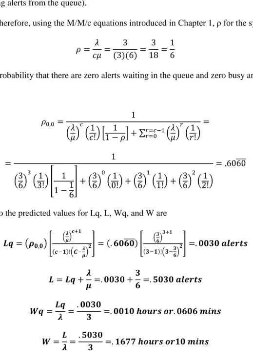
𝑳𝒒= �𝝆𝟎,𝟎� � �𝝀𝝁�𝒄+𝟏 (𝒄−𝟏)!�𝑪−𝝁𝝀�𝟐�= (.𝟔𝟎𝟔𝟎 ����)� �𝟑𝟔� 𝟑+𝟏 (𝟑−𝟏)!�𝟑−𝟑𝟔�𝟐�=.𝟎𝟎𝟑𝟎𝒂𝒍𝒆𝒓𝒕𝒔 𝑳= 𝑳𝒒+𝝁𝝀 =.𝟎𝟎𝟑𝟎+𝟑𝟔=.𝟓𝟎𝟑𝟎𝒂𝒍𝒆𝒓𝒕𝒔 𝑾𝒒= 𝑳𝒒𝝀 =.𝟎𝟎𝟑𝟎𝟑 =.𝟎𝟎𝟏𝟎𝒉𝒐𝒖𝒓𝒔𝒐𝒓.𝟎𝟔𝟎𝟔𝒎𝒊𝒏𝒔 𝑾=𝑳𝝀= .𝟓𝟎𝟑𝟎𝟑 =.𝟏𝟔𝟕𝟕𝒉𝒐𝒖𝒓𝒔𝒐𝒓𝟏𝟎𝒎𝒊𝒏𝒔 M/M/c Model Results
Figure 6 displays data from a run of the model with λ=3, μ=6, and c=3 analysts. The values of the four response variables converge to the analytically predicted values, which are marked by the red reference lines. Due to the relatively low density of the
system (ρ=1/6), convergence is not as complete as in the M/M/1 case above. Still, the model output agrees nicely with theoretical values.
Figure 6. For an M/M/3 system with λ=3 and μ=6, the model agrees with analytical predictions of the four response variables.
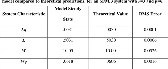
Table 3. Comparison of the average system dependent variable values output by the model compared to theoretical predictions, for an M/M/3 system with λ=3 and μ=6. System Characteristic
Model Steady State
Theoretical Value RMS Error
Lq .0031 .0030 0.0001
L .5031 .5030 0.0006
W 10.05 10.00 0.0526
Wq .0618 .0606 0.0016
M/M/1 with Priority Analytical Results
Now the model will return to a single analyst, but multiple alert priority levels will be added. To keep the calculations manageable, analytical results will be shown for two (2) priority levels, with λ2= 3, λ1= 2, μ = 12, and c = 1 where λ1 is high priority and
λ2 is low.
From the M/M/1 with Priority equations in Chapter 1, the first thing that must be calculated is the second moment of the service distribution, 𝑆𝑘2,
𝑆𝑘2 ���= 𝑛! 𝜇2 = 2! 122 = 1 72𝑜𝑟. 0139
which is plugged into the mean residual service time parameter,
𝑅� =12� 𝜆𝑘𝑆���𝑘2 𝑘 𝑘=1
=12�(3)�721�+ (2)�721��= .0347
The residual service time is used to estimate the average time spent in the queue for each priority level,
𝑊𝑞1 = 1− 𝜌𝑅� 2 = . 0347 1−122 = .0417 ℎ𝑜𝑢𝑟𝑠𝑜𝑟 2.500 𝑚𝑖𝑛𝑠 𝑊𝑞2 = (1− 𝜌 𝑅� 2)(1− 𝜌2− 𝜌1) = . 0347 �1−122� �1−122 −123� = .0714 ℎ𝑜𝑢𝑟𝑠𝑜𝑟 4.286 𝑚𝑖𝑛𝑠
then, the average amount of time any alert spends in the queue (the system-wide queue wait time) is calculated using a weighted approach,
𝑾𝒒= 𝝀𝟐𝑾𝝀𝒒𝟐+𝝀𝟏𝑾𝒒𝟏
𝟐+𝝀𝟏 =
(𝟑)(𝟒.𝟐𝟖𝟔) + (𝟐)(𝟐.𝟓)
𝟑+𝟐 =𝟑.𝟓𝟕𝟏𝒎𝒊𝒏𝒔
System sojourn time, W, is calculated for each priority level by adding the expected time the alert will wait in the queue plus the average time the alert takes to be serviced, 𝑊1 = 𝑊 𝑞1+1𝜇 = .0417 +�121�= .1250 ℎ𝑜𝑢𝑟𝑠𝑜𝑟 7.502 𝑚𝑖𝑛𝑠 𝑊2 = 𝑊 𝑞2+1𝜇= .0714 +�121�= .1547 ℎ𝑜𝑢𝑟𝑠𝑜𝑟 9.286 𝑚𝑖𝑛𝑠 and similarly to Wq, 𝑾= 𝝀𝟐𝑾𝝀𝟐+𝝀𝟏𝑾𝟏 𝟐+𝝀𝟏 = (𝟑)(𝟗.𝟐𝟖𝟔) + (𝟐)(𝟕.𝟓𝟎𝟐) 𝟑+𝟐 = 𝟖.𝟓𝟕𝟏𝒎𝒊𝒏𝒔
Finding the queue size for each alert priority level requires only a quick application of Little’s Law,
𝐿𝑞1 =𝜆
1𝑊𝑞1 = (2). 0417) = .0833 𝑝𝑟𝑖𝑜𝑟𝑖𝑡𝑦 1 𝑎𝑙𝑒𝑟𝑡𝑠
𝐿𝑞2 = 𝜆
2𝑊𝑞2 = (3)(.0714) = .2143 𝑝𝑟𝑖𝑜𝑟𝑖𝑡𝑦 2 𝑎𝑙𝑒𝑟𝑡𝑠
𝑳𝒒=𝑳𝒒𝟐+𝑳𝒒𝟏 =.𝟐𝟏𝟒𝟑+.𝟎𝟖𝟑𝟑=.𝟐𝟗𝟕𝟔𝒂𝒍𝒆𝒓𝒕𝒔
The system size, L, for each alert priority level is simply the number of alerts of that priority in the queue plus the average arrival rate,
𝐿1 =𝐿 𝑞 1 +𝜆1 𝜇 = .0833 + 2 12 = .2500 𝑎𝑙𝑒𝑟𝑡𝑠 𝐿2 =𝐿 𝑞 2 +𝜆2 𝜇 = .2143 + 3 12 = .4643 𝑎𝑙𝑒𝑟𝑡𝑠
Making the overall system size,
𝑳=𝑳𝒒+𝟏𝟐𝟑 +𝟏𝟐𝟐 =.𝟐𝟗𝟕𝟔+𝟏𝟐𝟑 +𝟏𝟐𝟐 =.𝟕𝟏𝟒𝟑𝒂𝒍𝒆𝒓𝒕𝒔
M/M/1 with Priority Model Results
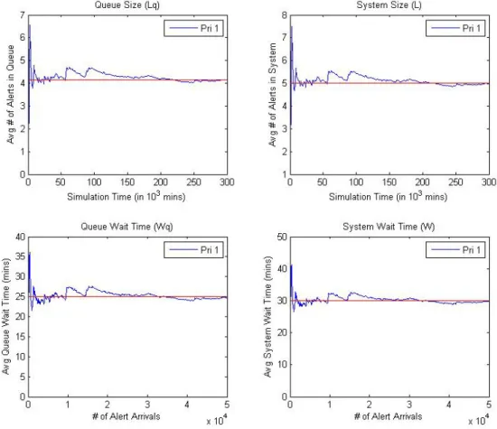
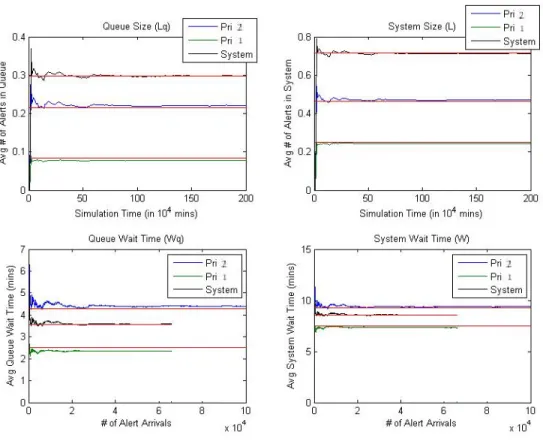
When using multiple priority levels, each level had its own value for Lq, L, Wq, and W but there was also a system value that looked at the characterization of the system as a whole without regard for priority levels. Figure 7 below shows the convergence of the model to the theoretical average values predicted above for each priority level as well as for the system as whole, which is shown in black. Red reference lines on the charts represent the closed-form analytical predictions.
One may notice that the Priority 1 and System curves do not extend the full length of the X axis in the Wq and W plots, whereas the Priority 2 curve does. This is simply a result of the way the model handles alert arrivals of differing priority levels. Since the total simulation length is determined based on a given number of arrivals for the lowest priority (in the case, Priority 2), the number of higher priority arrivals will vary based on its arrival rate. Since higher priority alerts generally arrive less frequently than low ones,
there will be less total high priority arrivals, but they will still enter the system throughout the entire simulated time span.
Figure 7. Model output for the four response variables for an M/M/1 with 2 Priority system. Red reference lines represent values predicted by analytical equations.
Table 4 compares the average values determined by the model to the theoretical values. For system-wide variables, error appears to be slightly less than for individual priority levels. As was seen for the M/M/3 system above, the higher error for the individual priority levels is influenced by the lower traffic density.
Table 4. Comparison of the model and theoretical dependent variable average values, both overall and for each priority level, in an M/M/1 with 2 priority level system.
System Characteristic Model Steady State Theoretical Value RMS Error
Lq .2976 .2976 0.0009 𝐿2𝑞 .2203 .2143 0.0067 𝐿1𝑞 .0774 .0833 0.0059 L .7123 .7143 0.0012 𝐿2 .4703 .4643 0.0068 𝐿1 .2420 .2500 0.0078 W 8.570 8.571 0.0054 𝑊2 9.374 9.286 0.1014 𝑊1 7.325 7.500 0.1732 Wq 3.592 3.571 0.0107 𝑊𝑞2 4.391 4.286 0.1174 𝑊𝑞1 2.341 2.500 0.1578 Assumptions
Many assumptions were made in the design and execution of the MATLAB queuing theory model. Some of the major assumptions were:
- All alerts that reach the queue are valid alerts and not the results of false positive triggers. All network traffic and detection activity that happens “upstream” from the
system is not included in the model, which starts at the alert queue and ends after the analyst services the alert.
- The network analyst is well-trained and has already traversed the steepest portion of the learning curve. In other words, the analyst is proficient at servicing alerts and spends only as much time as necessary on each one.
- In multiple server (i.e. multiple analyst) scenarios, each analyst has the same skill proficiency. In the real world, some analysts will have more advanced skills, so service times may vary drastically from analyst to analyst and may not be solely a function of the type of alert.
- There is assumed to be no collaboration between analysts. For example, the findings of one analyst does not affect the work of the others. Even though the alerts in service could have related root causes.
- The model does not allow alerts to be preempted. Alerts of the highest priority must wait at the front of the queue until an analyst finishes working on a lower priority alert. In the real world, a lower priority alert may be set aside when an exceptionally critical one arrives.
Summary
The method used in this research begins with validating the MATLAB model by comparing its results under simple conditions to the results predicted by closed-form analytical equations. Once the model is verified, its parameters are extended to simulate conditions beyond the reach of analytical equations. The results of these extensions and their interpretation are presented in the following chapter.
IV. Analysis and Results
Chapter Overview
This chapter introduces the modeling results for two different trial scenarios. In each scenario, 3D surface plots are generated to determine the sensitivity of the system to three key parameters: traffic density, number of analysts, and number of priority levels. The same set of traffic densities were used in both Scenario 1 and 2, ranging from lighter to heavier loads to see how the system would respond under varying amounts of stress. In Scenario 1 the model was executed across all traffic loads while varying the number of analysts from one (1) to three (3). In Scenario 2, the results of Scenario 1 under the three analyst case were extended using the same set of traffic loads, but with one (1), three (3), and five (5) priority levels.
Scenario 1: Varying the Number of Analysts
For the first scenario, the number of analysts was varied between one (1) , two (2), and (3) analysts across a range of traffic loads from lighter to heavier to determine the effect on average queue size (Lq), average system size (L), average queue wait time (Wq), and average system sojourn time (W). All values for alert arrival rate (λ) and alert service rate (μ) followed an exponential distribution.
Scenario1: Assumptions
For Scenario 1, the number of priority levels was fixed at three (one through three, with priority level one being high and priority three low) to make it easier to identify the sensitivity of the system to varying the number of analysts only, across a
range of traffic loads. The values for alert arrival rate (λ) and alert service rate (μ) for each priority level and traffic load are summarized in Table 5.
The base case for traffic load was created from assumptions about what would constitute reasonable arrival and service times for various types of alerts. Priority one alerts should be relatively rare events, so it is assumed that a priority one alert will only arrive on average once per 72-hour period, yielding λ=1/72. When they do occur, however, these events will require significantly more time to service since they pose a major risk to network operations and likely stem from complex or novel traffic
phenomena. In this scenario their service time was set to an average of three hours, or μ=1/3.
Priority two events will occur more frequently than priority one events, but less than the common priority three events, so they were set to arrive about once per 12-hour period, or λ=1/12. These events are assumed to take less time to service since they pose a lower risk to network operations and are likely simpler to analyze, so their service time was set at μ=1, or 1 alert per hour.
Finally, the common priority three alerts are generally considered low priority because they represent minimal risk to network operations. Since many can be dismissed without careful consideration, their average service time is quite quick, and has been assumed here as 10 minutes, or λ=6 alerts per hour.
To reduce and increase the traffic load, ρ=λ/μ, the base values described above for alert arrivals, λ, were decreased and increased by 25%, respectively, across all priority levels. As analysts were added to the system, the corresponding service capacity
automatically increased, so the lambda values were doubled or tripled as necessary to ensure the same stress was applied regardless of the number of analysts employed. Table 5. Summary of the model parameters used to generate each of the nine cases in Scenario 1.
Scenario 1: System-Wide Analysis
The output under Scenario 1 conditions for average system queue size (Lq), average system size (L), average system queue wait time (Wq), and average system sojourn time (W) are displayed in Figure 8.
Lambda Mu Rho Lambda Mu Rho Lambda Mu Rho
Pri 3 2.250 6.000 0.375 3.000 6.000 0.500 3.750 6.000 0.625
Pri 2 0.063 1.000 0.063 0.083 1.000 0.083 0.104 1.000 0.104
Pri 1 0.010 0.333 0.031 0.014 0.333 0.042 0.017 0.333 0.052
Sys Arrivals/Hr = Avg Serviced/Hr = Sys-wide Rho = Sys Arrivals/Hr = Avg Serviced/Hr = Sys-wide Rho = Sys Arrivals/Hr = Avg Serviced/Hr = Sys-wide Rho = 2.323 4.956 0.469 3.097 4.956 0.625 3.872 4.956 0.781
Lambda Mu Rho Lambda Mu Rho Lambda Mu Rho
Pri 3 4.500 12.000 0.375 6.000 12.000 0.500 7.500 12.000 0.625
Pri 2 0.125 2.000 0.063 0.167 2.000 0.083 0.208 2.000 0.104
Pri 1 0.021 0.667 0.031 0.028 0.667 0.042 0.035 0.667 0.052
Sys Arrivals/Hr = Avg Serviced/Hr = Sys-wide Rho = Sys Arrivals/Hr = Avg Serviced/Hr = Sys-wide Rho = Sys Arrivals/Hr = Avg Serviced/Hr = Sys-wide Rho = 4.646 9.911 0.469 6.194 9.911 0.625 7.743 9.911 0.781
Lambda Mu Rho Lambda Mu Rho Lambda Mu Rho
Pri 3 6.750 18.000 0.375 9.000 18.000 0.500 11.250 18.000 0.625
Pri 2 0.188 3.000 0.063 0.250 3.000 0.083 0.313 3.000 0.104
Pri 1 0.031 1.000 0.031 0.042 1.000 0.042 0.052 1.000 0.052
Sys Arrivals/Hr = Avg Serviced/Hr = Sys-wide Rho = Sys Arrivals/Hr = Avg Serviced/Hr = Sys-wide Rho = Sys Arrivals/Hr = Avg Serviced/Hr = Sys-wide Rho = 6.969 14.867 0.469 9.292 14.867 0.625 11.615 14.867 0.781
1 A
nal
ys
t
MINUS 25% TRAFFIC (Rho = .469) BASE CASE (Rho = .625) PLUS 25% TRAFFIC (Rho = .781)
2 A nal ys ts 3 A nal ys ts
Figure 8. System response in terms of Wq, Lq, W, and L with an increasing number of analysts under three different traffic loads.
Average system queue wait time (Wq) and average system sojourn time (W) decrease with an increasing number of analysts, across all traffic loads. The steepest gains in performance were seen at the heaviest tested traffic condition (ρ=.781), with a 43% decrease in Wq (from 116.1 to 49.8 minutes) moving from one (1) to two (2) analysts and a 53% decrease in Wq (from 49.8 minutes to 26.8) when moving from two (2) to three (3) analysts.
Interestingly, Lq and L were relatively unaffected by the number of analysts in the system, instead tracking primarily with increasing traffic load. The sensitivity to traffic load might be expected since an increase in alert arrivals at the same servicing capacity results in more total alerts in the system at a given moment. Lq and L do decrease slightly with the number of analysts, and Lq appears to be more sensitive to the number of analysts than L. At ρ=.469, moving from one (1) to three (3) analysts
decreased Lq by 74% (1.15 to .30 alerts), while L remained relatively stable at about 1.7 alerts. It should be noted that the sensitivity of Lq to the number of analysts decreased with increasing traffic load. At ρ=.781, Lq decreased by just 30% moving from one (1) to three (3) analysts (7.4 to 5.2 alerts), with L again experiencing very little movement, changing from 8.2 to just 7.5 alerts.
For the system as a whole, using a single analyst introduces a bottleneck which drives up all four response variables Wq, W, Lq, and L. Performance improvements from the employment of additional analysts stem from the creation of alternative paths through the system which alleviate bottleneck conditions. For instance, under the tested parameters, a single priority 1 alert takes an average of 3 hours to service. Therefore, in a single analyst system, when one of these alerts arrives, all other items in or entering the queue experience delays. The addition of more analysts provides alternative paths through the system for other alerts in the queue. It is unlikely that all analysts will be working priority 1 alerts at the same time due to their infrequent arrival rate.
Scenario 1: Analysis by Priority Level
In this section, the same four response variables (Wq, W, Lq, and L) are
discussed, but this time broken up by priority level to compare them to the system-wide responses discussed above.
Figure 9 shows the response variables for Priority 3 alerts, which can be seen to track very closely to the system-wide results. The reason for this is the frequent arrival rate and short service times of Priority 3 alerts, which makes them a frequent occurrence in the system. Their sheer frequency skews the system-wide results in their favor.
Figure 9. The four response variables (Wq, W, Lq, and L) for Priority 3 (low) alerts under Scenario 1 conditions. They track very closely to the system-wide results.
The situation is drastically different, however, when looking at the response of Priority 2 and Priority 1 alerts, shown in Figure 10 and Figure 11. The characteristic responses of Priority 1 alerts will be discussed specifically, but the same conclusions can be extended to Priority 2 results as well, since they demonstrate similar trends.
Figure 10. The four response variables (Wq, W, Lq, and L) for Priority 2 (mid) alerts under Scenario 1 conditions.
First, when looking at the average queue wait time for Priority 1 alerts, Wq_1, it is clear that Priority 1 alerts experience significantly reduced wait times compared to the system average. At ρ=.781 with one (1) analyst, Priority 1 alerts must only wait on average 21 minutes in the queue, compared to 116 minutes for the system. For the three (3) analyst case, Wq_1 drops to just 3 minutes, compared to nearly 27 minutes for the system. This stems from the rarity of Priority 1 alerts. The number of them expected to be in the queue, Lq_1, is extremely low (<<1) regardless of the number of analysts or
traffic load. The net result is that, with multiple analysts, Priority 1 alerts will almost always be the very first item in the queue upon arrival, and must only wait for an analyst to finish their current alert before being pulled from the queue and receiving service.
Figure 11. The four response variables (Wq, W, Lq, and L) for Priority 1 (high) alerts under Scenario 1 conditions.
As with Lq_1, L_1 is almost zero due to the infrequent occurrence of Priority 1 alerts, though it does increase slightly for an increasing number of analysts and increasing traffic load. This is simply due to the increased number of arrivals and increased
Interestingly, the average Priority 1 sojourn time, W_1, is nearly independent of both traffic load and number of analysts. This is driven by the short queue wait time for Priority 1 alerts, which means their time spent in the system is determined almost entirely by their average service time of 180 minutes.
Scenario 2: Varying the Number of Priority Levels
In the second scenario the focus was on determining how the alert priority scheme affected the response variables, both at the system level and by individual priority levels. Like Scenario 1, each response variable in Scenario 2 was examined under three different traffic loads, ρ=.469, .625, and .781.
The 3-analyst case with 3 priority levels from Scenario 1 was taken as the base case for Scenario 2. Three analysts were used due to their demonstrated performance advantages in Scenario 1. Then, the base case was transposed into similar 1-priority and 5-priority cases.
Care had to be taken when forming the 1-priority level case. To give the illusion of a single priority level while maintaining a distribution of arrival rates and service times on par with those from Scenario 1, there had to be alerts with different properties (i.e. different arrival rates and service times) but they had to enter the queue without priority. This had to be done by tweaking the model code slightly. The tweaked model allowed for the definition of multiple “priorities”, called Types in Table 6, with their own λ and μ values, but handled every Type of alert the same. In other words, all alerts had to start their journey through the system from the back of the queue.