Nonparametric and semiparametric methods for interval-censored failure time data

(1)

NONPARAMETRIC AND SEMIPARAMETRIC

METHODS FOR INTERVAL-CENSORED

FAILURE TIME DATA

A Dissertation

Presented to

the Faculty of the Graduate School

University of Missouri–Columbia

In Partial Fulfillment

of the Requirements for the Degree

Doctor of Philosophy

by

CHAO ZHU

Dr. (Tony) Jianguo Sun, Dissertation Supervisor

(2)

The undersigned, appointed by the Dean of the Graduate School, have

examined the dissertation entitled

NONPARAMETRIC AND SEMIPARAMETRIC

METHODS FOR INTERVAL-CENSORED

FAILURE TIME DATA

Presented by Chao Zhu

A candidate for the degree of Doctor of Philosophy

And hereby certify that in their opinion it is worthy of acceptance.

Dr. (Tony) Jianguo Sun

Dr. Nancy Flournoy

Dr. Tim Wright

Dr. Athanasios Micheas

(3)

(4)

ACKNOWLEDGEMENTS

I am greatly indebted to my dissertation supervisor, Dr. Tony Sun, for his kindly providing guidance throughout the development of this dissertation. His direction and comments have been of the greatest help at all times. This work could not have been done without him.

I am also very grateful for having an exceptional doctoral committee and wish to thank Drs. Nancy Flournoy, Tim Wright, Athanasios Micheas and Hong He for their continual support and constructive comments.

I extend many thanks to all persons in the Department of Statistics at the University of Missouri-Columbia for their helps during my graduate education, especially Zhigang Zhang, Qiang Zhao, Lianming Wang, Liuquan Sun and Xingwei Tong, for their useful discussions.

(5)

LIST OF TABLES

Table 1: Estimated Empirical Sizes and Powers of the Test Procedure (Chapter 2) 64

Table 2: Interval-censored HIV Infection Data (Chapters 2 & 3) . . . 65

Table 3: Interval-censored HIV infection Data (Chapters 2 & 3, continued) . . . .66

Table 4: Empirical Sizes of the Proposed Test Procedure (Chapter 3) . . . 67

Table 5: Empirical Powers of the Proposed Test Procedure (Chapter 3) . . . 68

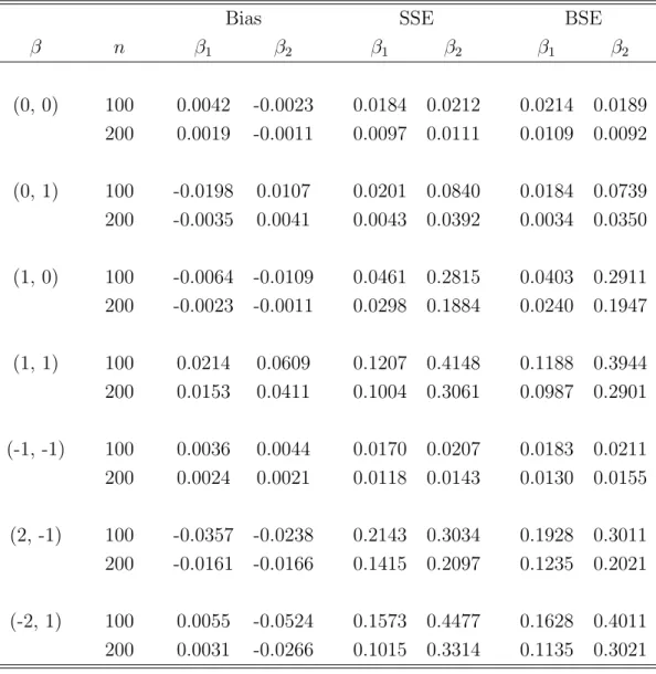
Table 6: Summary Statistics for the Numerical Studies (Chapter 4) . . . 69

(8)

LIST OF FIGURES

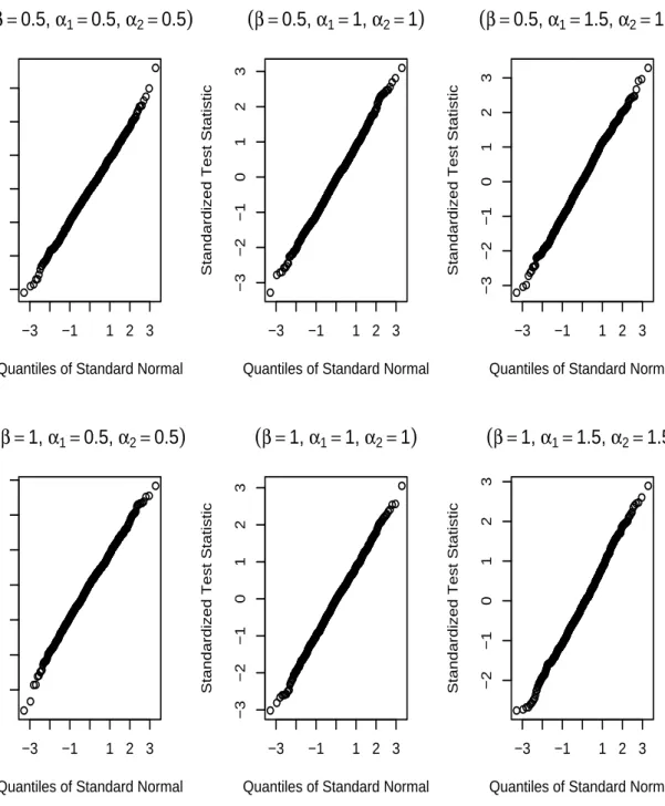
Figure 1: Normal Quantile Plots (Chapter 2) . . . 71

Figure 2: Estimated Log Odds Ratio for Two Groups (Chapter 2) . . . 72

Figure 3: Normal Quantile Plots for n= 50 (Chapter 3) . . . 73

Figure 4: Normal Quantile Plots for n= 100 (Chapter 3) . . . 74

Figure 5: Joint Empirical Distributions of Observation Times (Chapter 3) . . . 75

Figure 6: Joint Empirical Distributions of Observation Times (Chapter 3) . . . 75

Figure 7: Nonparametric Estimators of the Distribution Functions (Chapter 3) . . . .76

Figure 8: Survival Functions for β1 = 0 andβ2 = 1 (Chapter 4) . . . 77

Figure 9: Survival Functions for β1 = 1 andβ2 = 1 (Chapter 4) . . . 77

Figure 10: Survival Functions for β1 =−1 and β2 =−1 (Chapter 4) . . . 78

Figure 11: Survival Functions for β1 = 2 and β2 =−1 (Chapter 4) . . . 78

Figure 12: Normal Quantile Plots for β1 = 2 andβ2 =−1 (Chapter 4) . . . 79

(9)

NONPARAMETRIC AND SEMIPARAMETRIC METHODS FOR INTERVAL-CENSORED FAILURE TIME DATA

Chao Zhu

Dr. (Tony) Jianguo Sun, Dissertation Supervisor

ABSTRACT

Interval-censored failure time data commonly arise in follow-up studies such as clin-ical trials and epidemiology studies. For their analysis, what interests researcher most includes comparisons of survival functions for different groups and regression analysis. This dissertation, which consists of three parts, consider these problems on two types of interval-censored data by using nonparametric and semiparametric methods.

In Chapter 2, we discuss a goodness-of-fit test for checking the proportional odds (PO) model with interval-censored data. The PO model has a feature that allows the ratio of two hazard functions to be monotonic and converge to one. Hence, it provides an important tool for modeling the situation where hazard functions are nonproportional. We derive a procedure for testing the PO model, which is a generalization of Dauxois and Kirmani (2003) for right-censored data. Simulation studies suggest that the proposed test works well and we apply the test to a real dataset from an AIDS cohort study.

Chapters 3 considers nonparametric comparison of survival functions. For this, several test procedures have been proposed for interval-censored failure time data in which distri-butions of censoring intervals are identical among different treatment groups. Sometimes these distributions may not be the same and depend on treatments. A class of test statis-tics is proposed for situations where the distributions may be different for subjects in different treatment groups. The asymptotic normality of the test statistics is established and the test procedure is evaluated by simulations, which suggest that it works well. An illustrative example is provided.

(10)

data. For their regression analysis, One limitation of commonly used models is that they cannot be used to situations where survival functions cross. We consider a class of two-sample models that include these commonly used models as special cases and especially, are appropriate for crossing survival functions. Some estimating equation-based approaches are presented and the proposed estimates of regression parameters are shown to be consistent and asymptotically normally distributed. The method is evaluated using simulation studies and applied to a set of current status data arising from a tumorgenicity experiment.

(11)

CHAPTER 1 INTRODUCTION

1.1 Basic Quantities in Survival Analysis

Survival analysis, or time-to-event data analysis is used predominately in biomedical science where the interest is in observing time to death either of patients or of laboratory animals. It has also been used widely in social sciences where interest is on analyzing time to events such as job change, marriage, birth of children and so forth. The engineer-ing science has also contributed to the development of survival analysis which is called “reliability analysis” or “failure time analysis” in this field, where the main focus is on modeling the time of machines or electronic components to break down. The data arising from these fields are usually referred to as survival data, time-to-event data, or failure

time data. Note that the failure time, usually denoted by T, is a nonnegative random

variable.

The survival function of T is defined as S(t) = P(T ≥ t) = 1−F(t), where F(t) is the cumulative distribution function (CDF). S(t) is the probability that an individual experiences the event no earlier than time t. In survival analysis, the survival function of a failure time is preferred over the cumulative distribution function because it is more intuitive and easier to communicate with people in applied fields where survival data occur such as medical sciences.

(12)

function ofT are also commonly used in modelingT because of their conveniences. When

T is continuous, the hazard function of T is defined as

λ(t) = lim ∆t→0 1 ∆tP(t≤T < t+ ∆t|T ≥t) = f(t) S(t) =−[ d dt{S(t)}]/S(t),

where f(t) = dF(t)/dt is the density function of T. Note that λ(t) is the instantaneous failure rate at time t given that an individual survives up to time t−_{. The cumulative}

hazard function is defined as

Λ(t) = Z _t

0

λ(u)du.

It is easy to see that

S(t) = exp[−Λ(t)] = exp[−

Z _t 0

λ(u)du].

Thus,S(t), λ(t), or Λ(t) uniquely determines the distribution ofT.

IfT is a discrete random variable taking values 0 =t0 < t1 < t2· · ·, the hazard function is defined as

λ(tj) = P(T =tj|T ≥tj) =

f(tj)

S(tj)

, j = 1,2,· · ·

whereS(t0) = 1 andf(tj) =S(tj)−S(tj+1), j = 1,2,· · ·. The cumulative hazard function is defined as

Λ(t) = X

tj≤t

λ(tj).

1.2 Typical Censoring Mechanisms and Examples

Imagine that you are a researcher in a hospital for studying the effectiveness of a new treatment for a generally terminal disease. The major variable of interest could be the number of days (failure time T) that the patient with the disease survives. In principle,

(13)

if everyone dies, one could use the standard parametric and nonparametric statistics for describing the average survival and for comparing the new treatment with traditional treatments. However, at the end of the study there may be patients who survive over the entire study period, in particular among those patients who entered the hospital (and the research project) late in the study. Also there may be other patients with whom we lose contact. Surely, one would not want to exclude all of these patients from the study by declaring them to be missing (since most of them are “survivors” and, therefore, they reflect on the success of the new treatment method). These observations, which contain only partial information, are called censored observations (e.g., patient A survived at least 4 months before he moved away and we lost contact. The term censoring was first used by Hald, 1949).

Above is an example of right censoring. It is the most commonly encountered censoring mechanism in many fields such as clinical trials, environmental science, insurance, and

manufacturing. Two common types of right censoring are Type I and Type II censoring.

The Type I right censoring means that there is a fixed censoring time C and the exact

failure time X of an individual is known if and only if X is less than or equal to C. If X is greater than C, his or her event time is censored at C. The data from this type of experiments can be conveniently represented by pairs of random variables (T, δ), where δ

indicates whether the survival time is observed (δ= 1) or censored (δ= 0) andT is equal to X if the survival time is observed and C if it is censored, i.e., T =min(X, C).

Type II right censoring means that a study continues until r failures occur, where r is a predetermined integer (r < n). Experiments involving Type II censoring are often used in testing of equipment life. Here, all items are put on test at the same time and the test

(14)

is terminated when r of the n items have failed. Such an experiment may save time and money because it could take a very long time for all items to fail. Also the statistical treatment of Type II censored data is simpler in some sense because the data consist of

the r smallest survival times in a random sample of n survival times and the theory of

order statistics is directly applicable.

A failure time T associated with a specific individual in a study is considered to be left

censored if it is less than a censoring time Cl, that is, the event of interest has already

occurred for the individual before that person enters the study at time Cl. For such

individuals, we know that they have experienced the event some time before time Cl,

but their exact event time is unknown. For example, on a survey questionnaire, the investigator wonders when the individual first used marijuana. A subject is then left censored if he/she admits that he/she has used it before but cannot recall when the first time was.

Interval censoring is another type of censoring mechanism. There exist two types of

interval-censored data, case I and II interval-censored data (Groeneboom and Wellner,

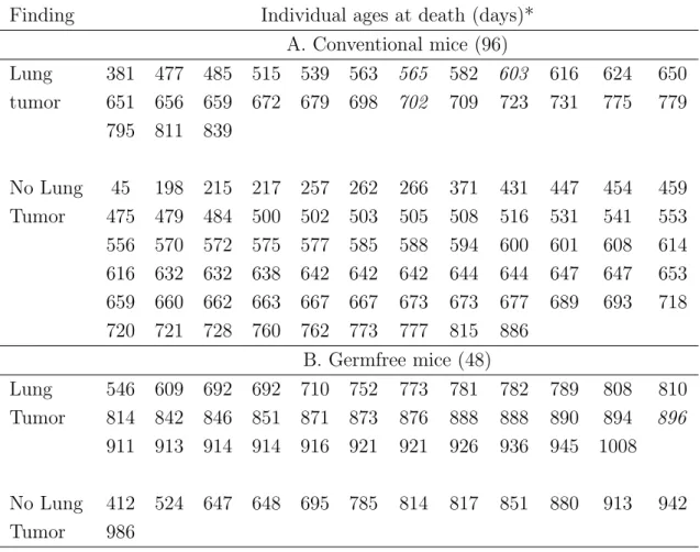
1992; Sun, 2005). The former, which is also often referred to as current status data, means that each subject is observed only once and thus the failure event of interest is observed only to have occurred before the observation time or not yet. In other words, the failure time of interestT is either left- or right-censored. Case I interval-censored data commonly occur in, for example, tumorigenicity experiments. In these experiments, the tumor onset time of animals is usually of main interest but not observable. Instead, only tumor status is usually known at death (either natural death or being sacrificed). Thus, the tumor onset time is known only to be less or greater than the death time.

(15)

Case II interval-censored data mean that the failure time T is known only to belong to an interval, say [L, R]. They reduce to case I interval-censored data if the interval includes either 0 or infinity. This type of data arises in many medical and health studies that entail periodic follow-ups. In this situation, an individual due for scheduled observations for a clinically observed change in disease status may miss some observations and may return with a changed status, thus contributing an interval-censored time of the occurrence of the change. Another example arises in the acquired immune deficiency syndrome (AIDS) studies that concern the human immunodeficiency virus (HIV) infection and the AIDS incubation time (the time from HIV infection to AIDS diagnosis). In this case if a subject is HIV positive at the beginning of the study, his or her HIV infection time is usually determined by a retrospective study of the subject’s history. Thus only an interval given by the last HIV negative test and the first HIV positive test is known for the HIV infection time.

Another way to represent a case II interval-censored observation is to use {U, V, δ1 = I(T ≤U), δ2 =I(U < T ≤V), δ3 = 1−δ1−δ2} assuming that each subject is observed

twice, whereU andV are two random variables satisfyingU ≤V with probability 1. This

formulation is convenient and often used, for example, in a theoretical investigation of an inference procedure. Both representations give rise to the same likelihood function. Note

that although (U, V) representation seems natural, it is not common to have

interval-censored data collected or given in these formats in practice. However, it is much easier

and more natural to impose assmptions such as independence with T on them than on

(L, R) representation, which is often needed for derivation of the asymptotic properties of inference procedures. For data given in (U, V) representation, one can easily obtain the

(16)

corresponding data with (L, R) representation. More discussion on this is given in later chapters.

1.3 Parametric and Semiparametric Models in Survival Analysis

In this section, we review some commonly used parametric and semiparametric models in survival analysis.

1.3.1 Parametric models

Parametric models (for the failure time T) naturally smooth the data by “borrowing”

information from adjacent points. With growing computing power and existing statis-tical programming languages, it is relatively simple to work with exact likelihood for interval-censored data with a variety of parametric models. Among other distributions, the exponential, Weibull and log-logistic distributions are mostly used in practice. We shall briefly introduce the latter two distributions in the following.

Suppose that T is continuous. By Weibull distribution, we mean that T has density

function

f(t) = α η tα−1 _exp_{−_{η t}α_}_,

where α >0 andη >0. Thus the survival function of T is

S(t) = exp{−η tα}

and the hazard function is

(17)

The corresponding cumulative hazard function is Λ(t) =

Z _t 0

α η tα−1_dt₌_{η t}α_.

Note that the Weibull distribution is flexible enough to accommodate increasing (α >

1), decreasing (α < 1), or constant (α = 1) hazard rates. When α = 1, the Weibull

distribution reduces to the exponential distribution with λ(t) = η.

A failure time T is said to follow the log-logistic distribution if its logarithm,Y =ln(T), follows the logistic distribution, a distribution closely resembling the normal distribution. Its survival function and hazard rate may be written as

S(t) = 1 1 +η tα

and

λ(t) = α η tα−1 1 +η tα.

The numerator of the hazard function is the same as the Weibull hazard, but the denom-inator allows the hazard to possess the following characteristics: monotone decreasing

for α ≤ 1, and for α > 1, the hazard rate increases initially to a maximum at time

[(α−1)/η]1/α _{and then decreases to zero as time approaches infinity.} 1.3.2 The proportional hazards model

Although the analysis of interval-censored data based on parametric models can be simple and efficient if the model is correctly specified, they are not widely used since the model choice is hard to determine in many situations. Instead, one usually looks for semiparametric or nonparametric methods. For the former, a common used model is the proportional hazards (PH) model, also referred to as the Cox model (Cox, 1972). It

(18)

specifies the hazard function of a continuous survival time T to have the form

λ(t|Z) = λ0(t) exp{β0Z}

given covariates Z which may depend on time, where β is a p×1 vector of unknown

regression parameters and λ0(t), the baseline hazard, is an unknown and unspecified

function. Note that the proportionality comes from the fact that, for example, if we look at two individuals with covariate valuesZ and Z∗_{, the ratio of their hazard functions is}

λ(t|Z) λ(t|Z∗₎ = λ0(t) exp[ P_p k=1βkZk] λ0(t) exp[ P_p k=1βkZk∗] = exp " _p X k=1 βk(Zk−Zk∗) # ,

which is a constant, where β = (β1, ..., βp). Usually β is of the main interest and can

be estimated independently by the partial likelihood approach (Cox, 1975) when right-censored data are observed. This appealing property of the PH model, together with its great flexibility, has made it one of the most popular models in survival analysis during the past three decades.

Diamond et al. (1986) were the first to use the PH model on case I interval cen-sored data. Their methods, however, require estimation of the baseline hazard λ0(t). Huang (1996a) gave a systematic treatment of the proportional hazards model under case I interval censoring. He showed that, under certain regularity conditions, ˆβn, the

max-imum likelihood estimator (MLE) of β, is consistent with an n1/2 _{convergence rate and} has an asymptotic normal distribution with the limiting variance given by the inverse of the Fisher information of β. However, ˆΛn, the MLE of the cumulative hazard function,

is only consistent with an n1/3 _{convergence rate, and its asymptotic distribution is} un-known. Finkelstein (1986) proposed to use the Newton-Raphson algorithm to compute

(19)

case II interval censoring. Satten (1996) proposed a marginal likelihood method to fit the proportional hazards model to case II interval-censored data, and Pan (2000) applied a multiple imputation approach for comparing two treatments. Betensky et al. (2002) proposed a local likelihood method mainly for estimating the baseline hazard function, while Cai and Betensky (2003) introduced piecewise linear penalized spline for the same purpose.

1.3.3 The proportional odds model

An important alternative to the PH model is the proportional odds (PO) model, which assumes that

log{F(t|Z)/S(t|Z)}=h(t) +β0Z,

where F(t|Z) and S(t|Z) denote the distribution function and the survival function of T

given Z, respectively, and h(t) is a baseline monotone-increasing function, also referred to as the baseline log odds. The original PO model was developed by McCullagh (1980) for analyzing ordinal data. Although this model is not as commonly used as the PH model when censored data are observed, partly due to the lack of a widely accepted estimation procedure for regression parameterβ, it does provide certain flexibility that the PH model can not. For instance, the initial effect of treatment, or the differences between stages of the disease at diagnosis, may diminish with time and the hazard functions of different groups of patients should become more similar. In this case, two hazard functions from different treatment groups are not proportional, but changing with time. Thus the assumption of the PH model, which requires a constant ratio for two hazard functions, is then violated. One of the earliest applications of the PO model on interval censoring was

(20)

given by Dinse and Lagakos (1983). Rossini and Tsiatis (1996) also discussed the fitting of this model to case I interval censoring with approximating the baseline log odds by step functions, thus obtaining consistent and asymptotic normal estimators forβ. Huang and Rossini (1997) and Rabinowitz et al. (2000) considered the sieve estimation and the approximated score function methods, respectively. For asymptotic properties and computation of the MLEs ofβ and h(t), see Huang and Wellner (1996).

1.4 Nonparametric Survival Analysis

In addition to the semiparametric models discussed in the previous section, nonparamet-ric methods for the analysis of survival data have also attracted much attention. Similar to the semiparametric methods, nonparametric methods do not require the knowledge of the underlying distribution of the failure time T. Hence it provides a flexible way to deal with the data in many practical situations. In this section, we review some classical problems that can be addressed by using nonparametric methods.

1.4.1 Nonparametric Estimation of a Survival Function

One of the basic research problems in survival analysis is the estimation of a survival function, for which numerous methods have been proposed under different censoring mech-anisms. For right-censored data, consider a survival study that consists of n independent subjects. LetS(t) denote the true survival function andt0 = 0 < t1 < t2 < . . . < tk+1 =∞ the observed failure times. Define

dj = the number of failures at tj,

(21)

cj = the number of subjects censored in [tj, tj+1),

tj1, . . . , tjcj =censored survival times in [tj, tj+1) j = 0,1, . . . , k.

The likelihood function is then proportional to

L= k Y j=0 ( [S(tj)−S(tj+)]dj cj Y r=1 S(tjr+) )

and the nonparametric maximum likelihood estimator (NPMLE) of S(t) is given by

Kaplan-Meier estimator ˆ S(t) = Y j|tj<t rj −dj rj

(Kaplan and Meier, 1958).

A closely related estimator of a survival function is given by ˜S(t) = exp{−Λ(˜ t)},where ˜

Λ(t) is the Nelson-Aalen estimator of the cumulative hazard function and has the form ˜ Λ(t) = X j:t(j)≤t dj rj (Nelson, 1972; Aalen, 1978).

For case I interval-censored data or current status data, suppose that F denotes the

CDF of the survival time of interest. Then the NPMLE of F can be shown to be equal

to the isotonic regression of {d1/n1, ..., dm/nm} with weights {n1, ..., nm}, where dj =

P

i∈SjI(Ti ≤ sj), nj = |Sj| and Sj denotes the set of subjects who are observed at sj,

j = 1, ..., m. Thus by using the max-min formula for an isotonic regression (Barlow et al., 1972), the NPMLE of F can be written as

ˆ Fn(sj) = max u≤j minv≥j( v X l=u dj/ v X l=u nj).

It can be shown that the above ˆFn is consistent. Furthermore, as n → ∞ and at

(22)

convergence rate depending on if the probability of observingT =t0 is zero or away from zero. Note that this is different than the usualn1/2_{-covergence rate. However, the integral} of ˆFn and its linear functionals can be shown to have asymptotic normal distribution with

n1/2_{-convergence (Huang et al., 1995 and Geskus, 1999). Anderson et al.(1995) utilized} this property and constructed a nonparametric test procedure based on the asymptotic normality for comparing two survival functions with case I interval-censored data.

For case II interval-censored data, suppose that observed data can be represented by

{Ii}ni=1, where Ii = [Li, Ri) is the interval observed to contain the unobserved survival

time associated with the ith subject. If Li = 0, we have a left-censored observation and

if Ri =∞, we have a right-censored observation. Let{sj}mj=0+1 denote the unique ordered elements of {0,{Li}ni=1,{Ri}in=1,∞}, αij be the indicator of the event [sj−1, sj)⊆ Ii and

pj =F(sj)−F(sj−1). Then the likelihood function of p= (p1, . . . , pm+1)

0 is proportional to L(p) = n Y i=1 {F(Ri)−F(Li)}= n Y i=1 ( m_X+1 j=1 αijpj)

and the problem of finding the nonparametric maximum likelihood estimator ofF becomes

that of maximizing L(p) with respect to p subject to P_jm₌₁+1pj = 1 and pj ≥ 0(j =

1, . . . , m+ 1)

To maximize L(p) with respect to p, a simple and common way is to use the

self-consistency algorithm proposed by Turnbull (1976). In this case, the estimator of pj can

be easily obtained by using the following equation on the pj:

pj = 1 n n X i=1 αijpj P_m₊₁ l=1 αilpl , f or j = 1, . . . , r .

(23)

Note that the above self-consistency algorithm can be seen as a special case of the EM algorithm. Although it is easy to implement, it has been known to have a slow convergence rate. Alternatively, Groeneboom and Wellner (1992) developed a convex minorant algorithm, which converges faster than the self-consistency algorithm. However, both algorithms are iterative and in fact, there is no closed form for the NPMLE of F.

1.4.2 Comparisons of Survival Functions

The comparison of survival functions is a major goal of many survival studies such as clinic trials. There usually exist two general approaches for the comparison. One approach is to use semiparametric regression techniques, and the other is to use nonparametric test procedures. In the first approach, treatment indicators are included in regression models as covariates. Then certain types of tests, such as the score test, can be developed to test whether or not the corresponding regression coefficients are zero. In the second approach, distribution free procedures are developed to compare survival functions. Most such procedures use the ranks of failure times instead of the actual failure times, and they assume that censoring time distributions are the same across treatment groups.

In the case of nonparametric comparisons for right-censored data, the log-rank test (Mantel 1966), a generalization of the Savage test (1956), is the most commonly used procedure. It can be shown that the log-rank test statistic is actually the same as the score statistic from the partial likelihood under the PH model. In other words, the log-rank test is the locally most powerful test. Other nonparametric test procedures include: the weighted log-rank tests (Gehan, 1965; Breslow, 1970; Peto and Peto, 1972; Harrington and Fleming, 1982) and the procedures based on the differences between weighted

(24)

Kaplan-Meier estimates (Pepe and Fleming, 1989). For the first class, different weights can be used to adjust the sensitivity of the tests to the difference between hazard functions over time. However, the test procedures in this class could have low power if the hazard functions cross. In the second class, the tests may not be sensitive to the hazard differences because they are based on the differences of estimated survival functions. Obviously, such tests would not be efficient if the survival functions cross.

Several nonparametric test procedures have been developed to compare failure time distributions for interval-censored data. In addition to the test derived by Anderson et al. (1995) as above, Sun (1996) developed a log-rank type test, which is a counterpart of the log-rank test used for right-censored data, and Pan (2000) proposed a two-sample test using a multiple imputation approach. Petroni and Wolfe (1994) considered procedures based on the differences between the estimated survival functions. Lim and Sun (2003) investigated three classes of procedures based on the differences between the estimated survival functions, estimated hazard functions, and estimated cumulative hazard func-tions, respectively, using different distance measures. Most existing procedures, such as those proposed by Sun (1996) and Petroni and Wolfe (1994), can be viewed as special cases of their approaches. However, for most nonparametric test procedures, the methods are ad-hoc and the asymptotic properties of the test statistics are unknown. Also, they do not reduce to the log-rank test, the locally most powerful test, in the case of right-censored data.

1.5 Outline

(25)

the goodness-of-fit test of the proportional odds model with interval-censored data. As mentioned in Section 1.3, the PH model is the most commonly used model for regression problems. However, this model has been found to be inappropriate for some data sets due to the fact that hazard functions from different treatment groups are not proportional, but changing with time. In contrast, the PO model has a feature that allows the ratio of two hazard functions to be monotonic and converge to one. Hence, it provides an important tool for modeling the situation above. Unfortunately, there are no methods available for checking the PO model with interval-censored data. Corresponding to this, a procedure for testing the PO model is derived and its performance is evaluated by a simulation study. In addition, the proposed test procedure is applied to a data set from an AIDS cohort study.

In Chapter 3, we consider the nonparametric comparison of two survival functions in the presence of unequal censoring. Most existing methods assume that the distribution of observation times for two samples are identical. However, there exist cases that the observation times may depend on the treatments (covariates). A comparison not account-ing for differences in observation times could seriously overestimate or underestimate the treatment difference. A new test procedure is thus established. Simulation studies are conducted to compare the proposed test with two other procedures. Finally, an applica-tion from an AIDS cohort study is provided for illustraapplica-tion.

Chapter 4 considers semiparametric regression analysis of two-sample current status data. In practice, there exist situations when the data provide evidence of crossing hazard functions. For example, a treatment could be effective in the long run but may have certain adverse effects during the early stage. In this situation, the hazard functions may

(26)

cross. The commonly used semiparametric models mentioned above do not accommodate such a crossing phenomenon. In this chapter, we describe a two-sample semiparametric model that can accommodate crossing survival functions. The parameters in this model are two summary parameters that represent the short-term and long-term hazard ratios respectively. The model includes the proportional hazards model and the proportional odds model as special cases. Simulation studies show that the estimators perform well. In addition, a real dataset from a carcinogenicity experiment is provided for illustration purpose.

This dissertation concludes with Chapter 5, which discusses several directions for future research.

(27)

CHAPTER 2 TESTING THE PROPORTIONAL ODDS MODEL FOR

INTERVAL-CENSORED DATA

2.1 Introduction

Consider a survival study that involves two independent survival variables T1 and T2 with continuous distributionsF1(t) andF2(t). The proportional odds (PO) model postu-lates that 1 − F2(t) F2(t) = eβ 1 − F1(t) F1(t) ,

whereβ is a constant. Defineφi(t) = (1−Fi(t))/Fi(t),i = 1,2. Then the PO model can

be rewritten as φ2(t) = α φ1(t), whereα = eβ. That is, the odds of the survival between the two samples are proportional to each other. Let λi(t) denote the hazard function

corresponding to Fi(t). Under the PO model, we have that

λ2(t) λ1(t)

= 1

1 + (α−1){1−F1(t)} ,

which is a monotonic function and converges to 1 as t → ∞.

The PO model is attractive in many situations. This is especially the case when the ratio of the two hazards are not proportional, but changing with time. One of such example is that treatment effect diminishes along with time. Many authors have discussed inference about the PO model (Dabrowska and Doksum, 1988; Huang and Rossini, 1997; Rossini and Tsiatis, 1996; Murphy, Rosssini and van der Vaart, 1997; Shen, 1998). In particular,

(28)

Dauxois and Kirmani (2003) developed a procedure for testing the PO model for two sample right-censored failure time data. For inference based on interval-censored failure time data, Huang and Rossini (1997) and Rossini and Tsiatis (1996) proposed some sieve estimation approaches. Huang and Wellner (1997) and Rabinowitz et al. (2000) considered the same problem and studied the full likelihood approach and an approximate conditional likelihood approach, respectively.

Let w1(t) andw2(t) be two positive known weight functions such that the ratiow1/w2 is an increasing function. Defineθij =

R_τ₂

τ1 wi(t)φj(t)dt, whereτ1 and τ2 are prespecified

constants such that τ1 < τ2 with Fi(τ1) > 0 and Fi(τ2) < 1, i, j = 1,2. To test the PO model or the hypothesis H0 : φ2(t) = α φ1(t) for all t > 0 and some α > 0 against H1 : φ2(t) and φ1(t) are not proportional, Dauxois and Kirmani (2003) proposed to use the statistic

q(w1, w2) = θ11θ22 − θ12θ21 (2.1) with replacing 1−Fi(t) by their Kaplan-Meier estimators. In the following, we generalize

the above test procedure to the interval-censored failure time data situation.

Interval-censored data have become common as described in Chapter 1. However, there does not seem to exist a procedure to test the PO model for interval-censored data. Note that in this case, the Kaplan-Meier estimator does not exist anymore and also due to the significant difference between right-censoring and interval-censoring, the theory developed in Dauxois and Kirmani (2003) cannot be directly generalized to

interval-censored data. For example, the Kaplan-Meier estimator has a √n convergence rate,

but the nonparametric maximum likelihood estimator of a survival function for

(29)

Geskus and Groeneboom (1999) showed that under some conditions, the linear functional of the nonparametric maximum likelihood estimator from interval-censored data still has the usual √n convergence rate.

In the following, we first discuss in Section 2.2 the generalization of the test procedure given in Dauxois and Kirmani (2003) to two sample interval-censored data situations and the related asymptotic theory is established. Note that although the idea behind the generalized test is straightforward, the implementation and the derivation of asymptotic properties of the test are not trivial due to complex structure of interval-censored data. Section 2.3 considers the testing of the hypothesis H0 against H1 using the theory given in Section 2.2 and two implementation procedures are presented. In Section 2.4, the test procedure given in the previous sections is generalized to situations where there exists

a categorical covariate or K different populations with K ≥ 2. Simulation results for

assessing the performance of the proposed method are reported in Section 2.5 and Section 2.6 applies the method to a set of interval-censored data arising from an AIDS study. The chapter concludes with some remarks in Section 2.7.

2.2 Asymptotic theory for two- sample interval-censored data

In this section, we first consider situations where only two sample interval-censored data are available forT1 andT2 defined above. By this, we mean thatTi is not observable

except for knowing that it belongs to some interval given by

{Ui, Vi,∆i1 =I(Ti ≤Ui),∆i2 =I(Ui < Ti ≤Vi)},

(30)

i = 1, 2. In the following, we assume that Ti is independent of (Ui, Vi) and the observed data are {Uij, Vij,∆(i1j),∆ (j) i2 , i= 1,2, j = 1, ..., ni}, where {Uij, Vij,∆(i1j),∆ (j)

i2 } are i.i.d. replicates of (Ui, Vi,∆i1,∆i2).

Now consider the testing of the hypothesis H0. Let ˆFi(t) denote the nonparametric

maximum likelihood estimator of Fi(t) based on the interval-censored data

{Uij, Vij,∆(i1j),∆ (j) i2 ;j = 1, ..., ni} and define ˆ φi(t) = 1−Fˆi(t) ˆ Fi(t) , i= 1,2.

Motivated by the statistic given in equation (2.1), we propose to base the test on the statistic Qn(w1, w2) = ³_n 1n2 n ´₁_/₂ h ˆ θ11θˆ22−θˆ12θˆ21 i , (2.2) where n = n1 + n2 and ˆ θru = Z _τ₂ τ1 wr(t) ˆφu(t)dt , r = 1,2, u= 1,2.

It is easy to see that if the hypothesisH0 is true,Qn(w1, w2) should be close to zero. Thus H0 should be rejected in favor of the hypothesisH1 if |Qn(w1, w2)| is too large.

To employ the statistic Qn, we need to establish its asymptotic distribution under

the hypothesis H0. For this end, let Gi(u, v, δi1, δi2) denote the distribution function of (Ui, Vi,∆i1,∆i2) and hi(u, v) the density function of (Ui, Vi) with the marginal density

functions hi1 and hi2 forUi and Vi, respectively. Define

C1(t) =

(31)

and

C2(t) =

θ21w1(t)−θ11w2(t) F2(t)2

.

Also let ΨFi denote the solution to the following Fredholm integral equation

ΨFi(t) =di(t) ½ Ci(t)− Z _τ₂ τ1 ΨFi(t)−ΨFi(s) |Fi(t)−Fi(s)| h∗ i(t, s)ds ¾ , i= 1,2, (2.3) wheredi(t) =Fi(t)(1−Fi(t))/[hi1(t)(1−Fi(t)+hi2(t)Fi(t)] andhi∗(t, s) = hi(t, s)+hi(s, t). Also define Φi(u, v, δi1, δi2) = −δi1 ΨFi(u) Fi(u) −δi2 ΨFi(v)−ΨFi(u) Fi(v)−Fi(u) + (1−δi1−δi2) ΨFi(v) 1−Fi(v) .

Assume that the regularity conditions (A)-(D) of Fang, Sun and Lee (2002) hold about the random monitoring times (Ui, Vi) (i= 1,2). Then the asymptotic normality ofQn(w1, w2) is given in the following theorem.

Theorem 2.1. Assume that the weight functionswi(t) (i= 1,2)have bounded derivatives on [τ1, τ2] and n1/n → ρ (0 < ρ < 1) as n → ∞. Then under the above conditions and H0, Qn(w1, w2) has an asymptotic normal distribution with mean zero and variance

σ2 _{= (1}₋_ρ₎ Z Φ2 1(u, v, δ11, δ12)dG1(u, v, δ11, δ12) +ρ Z Φ2 2(u, v, δ21, δ22)dG2(u, v, δ21, δ22). (2.4)

The proof of this theorem is sketched in the Appendix. In the next section, we describe the use of the results given above for testing H0.

(32)

To test the hypothesis H0 by using the statistic Qn, we present two implementation

approaches based on the above theorem. One is to directly apply Qn by deriving a

consistent estimate of the asymptotic variance σ2 _{and the other is to employ a simple}

bootstrap procedure.

First we consider estimation of σ2_{. For this, note that ˆ}_F

i (i = 1,2) only has mass at

observation times and according to Theorem 3.5 of Groeneboom (1996), Ψ_Fˆ_i is absolutely continuous with respect to ˆFi and a step function with jumps at the time points where

ˆ

Fi jumps. Let 0 < t(1i) < ... < tm(i)i < ∞ denote the time points at which ˆFi has jumps

and z(_ji) = ˆFi(t(ji)), i = 1,2,j = 1, ..., mi. Also let ˆHi, ˆHi1 and ˆHi2 denote the empirical distributions of (Ui, Vi),Ui and Vi, respectively. Define

∆j(hil) = Z _t(i) j+1 t(ji) hil(t)dt≈ Z _t(i) j+1 t(ji) dHîl(t), l= 1,2, ∆jk(hi) = Z _t(i) j+1 u=t(ji) Z _t(i) k+1 v=t(_ki) hi(u, v)dudv≈ Z _t(i) j+1 u=t(ji) Z _t(i) k+1 v=t(_ki) dHî(u, v), d(_ji) = z (i) j (1−z (i) j ) ∆j(hi1)(1−zj(i)) + ∆j(hi2)zj(i) , ∆j(Ci) = Z _t(i) j+1 t(_ji) dCi(t)dt ≈ Z _t(i) j+1 t(_ji) dCî(t) j, k = 1, ..., mi, i = 1,2, where ˆ C1(t) = ˆ θ12w2(t)−θˆ22w1(t) ˆ F1(t)2 , Cˆ2(t) = ˆ θ21w1(t)−θˆ11w2(t) ˆ F2(t)2 .

Lety(_ji)= Ψ_Fˆ_i(t(ji)). Then it can be shown that the vector y(i) = (y(1i), ..., ym(i)i)0 (i= 1,2) is

the unique solution to the following set of linear equations

y(_ji) ( (d(_ji))−1₊X k<j ∆kj(hi) z_j(i)−z(_ki) + X k>j ∆jk(hi) z(_ki)−z_j(i) ) = ∆j(Ci)+ X k<j ∆kj(hi) z_j(i)−z_k(i)y (i) k + X k>j ∆jk(hi) z_k(i)−z_j(i)y (i) k

(33)

For each i, define ˆ Φi(u, v, δi1, δi2) =−δi1 Ψ_Fˆ_i(u) ˆ Fi(u) −δi2 Ψ_Fˆ_i(v)−Ψ_Fˆ_i(u) ˆ Fi(v)−Fˆi(u) + (1−δi1−δi2) Ψ_Fˆ_i(v) 1−Fˆi(v) .

It follows from the uniform consistency of ˆHi, ˆHi1, ˆHi2 and ˆFi that ˆΦi(u, v, δi1, δi2) is a uniformly consistent estimator of Φi(u, v, δi1, δi2). This naturally yields a consistent estimator of σ2 _{given by} ˆ σ2 = n2 n Z ˆ Φ2₁(u, v, δ11, δ12)dGˆ1(u, v, δ11, δ12) + n1 n Z ˆ Φ₂2(u, v, δ21, δ22)dGˆ2(u, v, δ21, δ22), (2.5) where ˆGi is the empirical estimator of Gi. Hence the test of the hypothesis H0 can be carried out by using the statisticQn(w1, w2)/σˆbased on the standard normal distribution. Note that the above estimator ˆσ2 _{is very technically involved due to the complexity of}

the estimator Ψ_Fˆ_i. Thus the above procedure could be complicated and demanding in

computation, especially when the number of jumps of ˆFi is not small. For this, we suggest

the following simple bootstrap procedure.

LetM be a prespecified integer and Q(0)n denote the observed value of the test statistic

Qn. For each i (= 1,2) and l (1 ≤ l ≤ M), draw a simple random sample

D_i(l) = {U_ij(l), V_ij(l),∆(_i₁jl),∆_i(₂jl), j = 1, ..., ni}

with replacement from the observed data on Ti. Let Q(nl) denote the value of statistic

Qn calculated based on the generated data set{D(1l), D2(l)}. It follows from the theorem

given in the previous section that under H0 and when n is large, the bootstrap samples

{Q(nl); l = 1, ..., M} follow a normal distribution. The variance of Q(0)n can then be

estimated by the sample variance, say ˆσ2

b, of the Q

(l)

n ’s and the hypothesis H0 can be

(34)

Similar bootstrap procedures have been used by Fang, Sun and Lee (2002) and Monaco, Cai and Grizzle (2005) among others.

To implement the above test procedure, one needs to determine the maximum likelihood estimator ˆFi of Fi. For this, several procedures are available (Gentleman and Geyer,

1994; Sun, 2004) and perhaps the simplest procedure, which will be used below, is the self-consistency algorithm given in Turnbull (1976). Also one needs to choose τ1 and τ2 and it is easy to see that to testH0 againstH1 over all possible t, one should select them to make the interval [τ1, τ2] as large as possible. Dauxois and Kirmani (2003) suggested to choose them such that

0 < Fˆi(τ1) < 10−3 , 0 < 1−Fˆi(τ2) < 10−3,

i = 1,2. Another choice that one has to make is the selection of weight functions w1 and w2 and different weight functions give different test statistics. It is apparent that these weight functions set up the measurement scales for the null hypothesis. If the null hypothesis is true, the test statistic Qn should be close to zero no matter what scales are

used and otherwise,Qnis away from zero. For the following numerical studies, we consider

several choices including the natural and simple functionsw1(t) = 1 andw2(t) = 1/(1+t). It should be noted that in practice, interval-censored data may be given in the form

{(Lij, Rij], i = 1,2, j = 1, ..., ni}, where (Lij, Rij] is the interval within which the failure

time of the jth subject from the ith group is observed to occur. This form is commonly used in practice, while the form used above is more convenient and usually used for the situation where the asymptotic property of an approach for interval-censored failure time data is of interest. There is no difference between the two forms in terms of implementation of the test procedure proposed here and other inference procedures (Huang and Wellner,

(35)

1997).

2.4 K- sample test procedure

Now we consider situations where study subjects come from K different populations.

Let Tij denote the survival variable of interest from subject j in population i with the

cumulative distribution Fi(t),j = 1, ..., ni,i = 1, ..., K. As before, define

φi(t) =

1 − Fi(t)

Fi(t)

, i = 1, ..., K

and suppose that one is interested in testing the null hypothesisH0

0 versus the alternative hypothesis H0

1, where H0

0 : φi(t) = αiφ1(t) for allt >0 and some constants αi >0, i = 2, ..., K,

H0

1 : someφi(t) and φ1(t) are not proportional.

Furthermore, suppose that for theTij’s, only interval-censored data are available and have

the form

{Uij, Vij,∆(i1j),∆

(j)

i2 ; j = 1, ..., ni, i= 1, ..., K}

as before, where ∆_i(₁j) = I(Tij ≤ Uij), ∆i(2j) = I(Uij < Tij ≤ Vij). In the following, it is

assumed that Tij is independent of (Uij, Vij).

As before, let ˆFi(t) denote the nonparametric maximum likelihood estimator of Fi(t)

based on the interval-censored data {Uij, Vij,∆(ij1),∆

(j) i2 ; j = 1, ..., ni} and define ˆ φi(t) = 1−Fˆi(t) ˆ Fi(t) , θˆrk = Z _τ₂ τ1 wr(t) ˆφk(t)dt ,

i, r, k = 1, ..., K. In the above, τ1 and τ2 are defined as in the previous sections and the wr(t)’s are some positive known weight functions such that w1/wr is an increasing

(36)

function. To testH0

0 versusH10, as in Section 2.2, we propose to use the statisticQn(w) =

(Q(2)n (w1, w2), ..., Q(nK)(w1, wK))0, where w = (w1, ..., wK)0 and Q(_ni)(w1, wi) = ³_n 1ni n ´₁_/₂ ³ ˆ θ11θˆii − θˆ1iθˆi1 ´

with n = PK_i₌₁ ni. It is apparent that if H00 is true, all Q

(i)

n (w1, wi) should be close to

zero.

For the null asymptotic distribution of Q_n(w), following the notation used in the pre-vious sections, let Gi(u, v, δi1, δi2) denote the distribution function of (Ui1, Vi1,∆(1)i1 ,∆

(1)

i2 ) and hi(u, v) the density function of (Ui1, Vi1) with the marginal density functions hi1 and hi2 for Ui1 and Vi1, respectively, i= 1, ..., K. Define

Ci1(t) = θ1iwi(t)−θiiw1(t) F1(t)2 , Ci2(t) = θi1w1(t)−θ11wi(t) Fi(t)2 .

Also let Ψi1 and Ψi2 denote the solutions to the Fredholm integral equations

Ψi1(t) = d1(t) ½ Ci1(t)− Z _τ₂ τ1 Ψi1(t)−Ψi1(s) |F1(t)−F1(s)| h∗₁(t, s)ds ¾ and Ψi2(t) = di(t) ½ Ci2(t)− Z _τ₂ τ1 Ψi2(t)−Ψi2(s) |Fi(t)−Fi(s)| h∗_i(t, s)ds ¾ , respectively, where h∗ i(t, s) = hi(t, s) +hi(s, t) and di(t) = Fi(t)(1−Fi(t)) hi1(t)(1−Fi(t)) +hi2(t)Fi(t) . Also define Φi1(u, v, δ11, δ12) = −δ11 Ψi1(u) F1(u) −δ12 Ψi1(v)−Ψi1(u) F1(v)−F1(u) + (1−δ11−δ12) Ψi1(v) 1−F1(v) and Φi2(u, v, δi1, δi2) = −δi1 Ψi2(u) ₋_δ i2 Ψi2(v)−Ψi2(u) _{+ (1}₋_δ i1−δi2) Ψi2(v) _,

(37)

and assume that the regularity conditions (A)-(D) of Fang, Sun and Lee (2002) hold about the random monitoring times (Uij, Vij) (i = 1, ..., K, j = 1, ..., ni). Then one can

generalize the theorem 2.1 as follows.

Theorem 2.2Assume that the weight functionswi(t) (i= 1, ..., K)have bounded deriva-tives on [τ1, τ2] and ni/n →ρi (0< ρi <1) as n→ ∞. Then under the above conditions and H0, Qn(w) converges in distribution to a normal random vector with mean zero and a covariance matrix Σ = (σij), i, j = 2, ..., K, where

σii=ρi Z Φ2_i₁(u, v, δ11, δ12)dG1(u, v, δ11, δ12) +ρ1 Z Φ2_i₂(u, v, δi1, δi2)dGi(u, v, δi1, δi2), and for i6=j, σij = (ρiρj)1/2 Z Φ2 i1(u, v, δ11, δ12)dG1(u, v, δ11, δ12).

The proof of the theorem given above is similar to that of the theorem 2.1 and thus

omitted. Based on this theorem, one can carry out the test of H0

0 using the statistic

Q(w) ˆΣ−1_Q0₍_w_{), where ˆ}_{Σ is a consistent estimator of Σ. For the implementation, as in}

Section 3, one can easily develop a simple bootstrap procedure similar to that described for the two sample situation.

2.5 Numerical Studies

This section reports some results obtained from simulation studies conducted for as-sessing the performance of the proposed approach for testing the PO model. In the study, we focused on the two sample situation and to generateT1 and T2, the log-logistic

(38)

distributions F1(t) = F(1, β1) and F2(t) = F(α, β2) were used, where F(α, β) = (t/α)

β

1 + (t/α)β

andαandβ are constants. This givesφ2(t)/φ1(t) = αβ2tβ1−β2 andH0 andH1 correspond to β1 = β2 and β1 6= β2, respectively.

For censoring intervals, we mimicked interval-censored data commonly arising from periodic follow-up studies and first generated a right-censoring timeCij from the uniform

distribution U(0, A), where A is a positive constant chosen to control the percentage of right-censored observations. Given Cij, if Tij, the above generated failure time for the

jth subject from group i, is greater than Cij, we defined Lij = Cij and Rij = ∞.

That is, Tij was right-censored. If Tij ≤ Cij, we defined Lij = max(0, Tij −a1) and Rij = min(Tij+a2, Cij), wherea1 and a2 are random numbers generated independently from the uniform distributionU(0, B). HereBis a positive constant controlling the length of censoring intervals. For the variance estimation ofQn, the simple bootstrap procedure

was used and in the study, we tookτ1 andτ2 to be the smallest and largest possible values.

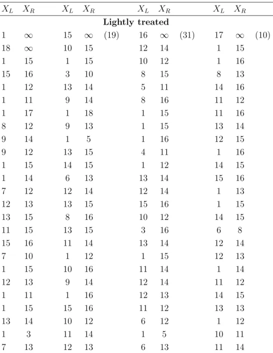
Table 1 presents the estimated size and power of the test procedure based on Qn for

testingH0 at the significance level of 5% based on 1000 replications,M = 500,n1 = 100, n2 = 150, w1(t) = 1 and w2(t) = 1/(1 +t). Here we considered the situations with α = 2, β1 = 1, 1.5, 2, or 3, β2 = 1, and the percentage of right-censored observations

being 10%, 20% or 30%. The top half of the table is for the case where B = 0.5 and

the bottom half is for the case whereB = 1. The results suggest that the test procedure seems to have right size and reasonable power. As expected, the power decreases when the length of censoring intervals increases.

(39)

sample size and weight function, we also performed simulations using different sample sizes and weight functions. For example, under the same set-up as in Table 1 but with

n1 = 200 andn2 = 300, we obtained powers of 0.610, 0.467 and 0.403 for the situations

with β1 = 1.5, B = 1, and 10%, 20% and 30% right-censorings, respectively. For the

exact same situation but with n1 = 100, n2 = 150, w1(t) = t and w2(t) = 1/(1 +t), the test gave powers of 0.398, 0.284 and 0.231, respectively. These results indicate that as expected, the power of the test procedure increases as the sample size increases and could depend on the selection of weight functions.

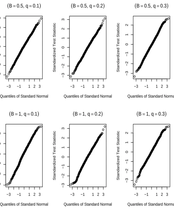
To evaluate the normal approximation given in Theorem, we studied the normal quan-tile plots of the standardized test statistics. Figure 1 displays such plots for B = 0.5

and 1 with α = 2, β1 = β2 = 1 under 10%, 20% and 30% right censoring percentages,

respectively. They suggested that the normal approximation works well.

2.6 An Application

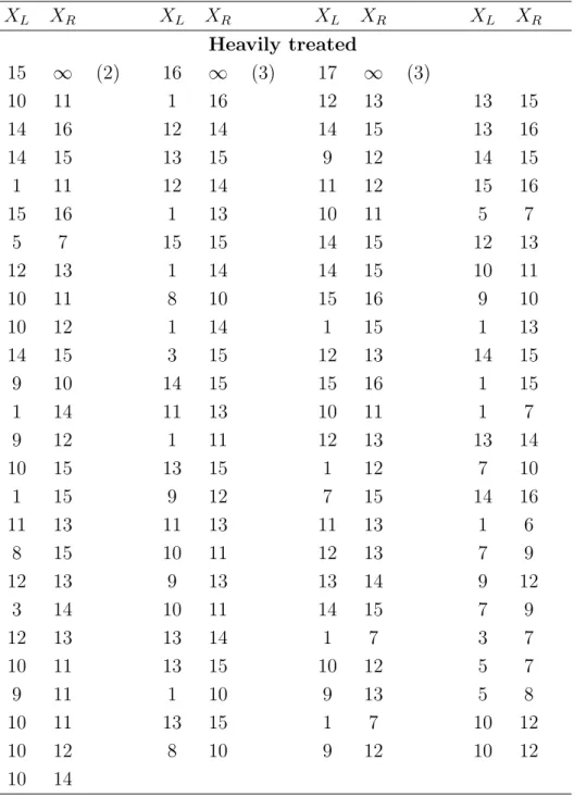
To illustrate the proposed methodology, consider the data presented in Tables 2 & 3, which are reproduced from DeGruttola and Lagakos (1989). The data arose from a cohort study on hemophiliacs that consists of 262 persons with hemophilia treated since 1978. All patients were at the risk of being infected by HIV due to contaminated blood that they received for their hemophilia. By the end of study, 197 subjects were confirmed to be infected with HIV and among these infected subjects, 25 were found infected at their first tests for the infection. Since the determination of HIV infection was based on periodic blood test results, only interval-censored data were obtained for the infection times. One objective of the study was to investigate the relationship between their HIV infection rate

(40)

and the amount of blood that they received.

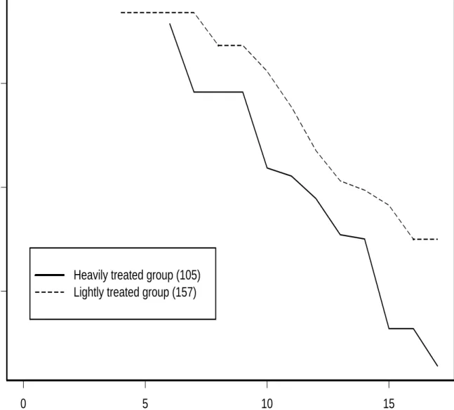
For this, in the original study, the patients were classified into two groups as the lightly and heavily treated groups. In the former group (157), the patients received less than 1000 µg/kgin each year and in the other group (105), the patients received at least 1000

µg/kg of blood for at least one year between 1982 and 1985. In the study, the observed time intervals for the HIV infection were measured in 6-month intervals.

Define T1 and T2 to be the times to HIV infection for the patients in the lightly and heavily treated groups, respectively. To examine the appropriateness of the PO model for the data set and the relationship of the distribution functions of T1 and T2, we applied the test procedure proposed in the previous sections and obtained Q(0)n = 9.5547 with

the estimated standard error being 9.3053. In the procedure, we used w1(t) = 1 and

w2(t) = 1/(1 +t). This yielded ap-value of 0.305 for testing H0 againstH1 and suggests

that the PO model seems to be appropriate for the data. By using w1(t) = t and

w2(t) = 1/(1 +t), we obtained a p-value of 0.384 and the same conclusion. For the results, we tookτ1 = 6 andτ2 = 17, the smallest and largest possible time points forT2. To further investigate the fit of the PO model to the problem, we obtained the estima-tors of the separate log odds ratio functions, log ˆφi(t), corresponding to the two groups

and they are presented in Figure 2. Note that if H0 is true, the two curves should be

roughly parallel to each other. Figure 2 again suggests that the PO model seems to fit the data well.

2.7 Concluding Remarks

(41)

interval-censored failure time data. The analysis of interval-interval-censored data has recently attracted a lot of attention and several models including the PO model have been investigated for their regression analysis. However, there seems to exist little research in the literature on the development of formal approaches that can be used for model checking. One reason is that the censoring mechanism involved in interval-censored data is much more difficult to deal with than that in right-censored data in addition to less information given by the interval-censored data. This can be seen from the problem considered here. The simulation results suggested that the procedure given here seems to perform reasonably well for practical situations.

Although the focus here is on K sample situations, the test procedure proposed in

the previous sections can be applied to situations with categorical covariates. However, it does not seem to be straightforward to generalize the idea used here to continuous covariate situations, for which some different test procedures need to be developed for testing the PO model. Another important question that was not fully discussed in the previous sections is the selection of optimal weight functions for a given situation. As usual, this is a very difficult question (Sengupta, Bhattacharjee and Rajeev, 1998) and the existence of interval-censoring makes it even more challenging. Of course, one may first need to ask the existence of such weight functions, for which we have no clear answer. One other direction for future research is the asymptotic validity of the simple bootstrap procedure described in Section 2.3. Note that as mentioned before, several authors used similar procedures (Fang, Sun and Lee, 2002; Monaco, Cai and Grizzle, 2005), but no theoretical justification was given. Although the simulation study indicates that it works well, it would be helpful and desirable to provide some justifications.

(42)

CHAPTER 3 A NONPARAMETRIC TEST FOR INTERVAL-CENSORED DATA

WITH UNEQUAL CENSORING

3.1 Introduction

As discussed in Chapter 1, one of the primary objectives in clinical trials and epidemi-ological studies is to compare survival functions. In this case, one usually prefers to apply nonparametric methods due to the lack of knowledge about the underlying distributions of the failure time of interest. In this chapter, we consider such nonparametric compar-ison problems when only interval-censored failure time data are available. For survival comparison based on interval-censored data, a few test procedures have been proposed (Finkelstein, 1986; Self and Grossman, 1986; Fay, 1996; Pan, 2000; Petroni and Wolfe, 1994; Zhang et al., 2001, 2003; Zhao and Sun, 2004). However, most of them assume that censoring intervals or observation times for all subjects have the same distribution function, which obviously may not be true in practice. A failure to take into account this difference in distributions could seriously overestimate or underestimate the treatment difference. One exception is given by Sun (1999), who considered survival comparison based on case I interval-censored data when the distributions of observation times differ among different treatment groups.

In the following, we discuss the same problem as that in Sun (1999) for case II interval-censored data. Specifically, we consider the two-sample survival comparison problem and a

(43)

class of test statistics is presented in Section 3.2 that allow the distributions of observation times to be different between two treatment groups. The statistics are constructed based on linear functionals of estimated survival functions and are generalizations of those used in Zhang et al. (2001). The asymptotic normality of the test statistic is established. Monte Carlo simulation studies are performed to evaluate the finite sample properties of the proposed approach in Section 3.3 and Section 3.4 applies it to an AIDS cohort study. Some concluding remarks are given in Section 3.5.

3.2 Statistical Methods

Consider a survival study that consists ofn independent subjects randomly assigned to one of two treatments. For subjecti, letTi denote the failure time of interest and assume

that only an interval-censored observation on it is available. Specifically, suppose that the observed information includes two random variables Ui and Vi with Ui ≤ Vi and the

indicator variables δ1i = I(Ti ≤ Ui), δ2i = I(Ui < Ti ≤ Vi) and δ3i = 1 − δ1i − δ2i,