Debiased Post Selection Inference
byJingshen Wang
A dissertation submitted in partial fulfillment of the requirements for the degree of
Doctor of Philosophy (Statistics)
in the University of Michigan 2019
Doctoral Committee:
Professor Xuming He, Chair Professor Matias D. Cattaneo Assistant Professor Gongjun Xu Professor Ji Zhu
ACKNOWLEDGMENTS
I would like to first thank my advisor Xuming He for his support, patience, and guidance during the past years. Xuming’s rigor and incisiveness on research have profoundly influenced my way of approaching statistical problems. I will greatly miss our conversations, meetings, and phone calls, which were not only fun but also influenced my perception on academia and personal life.
I would like to thank Gongjun Xu for the helpful discussions on my work. Gongjun’s seemingly unlimited availability to meet and to discuss any questions were in fact indispensable to me. I am immensely grateful to Matias Cattaneo for many helpful advice and discussions during my job search process. Matias is not only an exemplary researcher, a motivating teacher and a caring mentor, but also an inspirational person who always has abundance of positive energy around. I would like to thank Rocio Titiunik for sharing her experience in personal and academic lives with me. The power in Rocio’s words gives me the confidence to overcome unforeseen challenges in the future. I would like to express my deep gratitude to Ji Zhu for bringing me to Michigan and giving me this wonderful PhD journey in the department. I would also specially thank my dear friend Xinwei Ma for many interesting discussions on diverse research topics. Finally, I would like to acknowledge my beloved parents and Alexander Giessing for their unwavering support in my life.
TABLE OF CONTENTS
Dedication . . . ii
Acknowledgment . . . iii
List of Figures . . . vi
List of Tables . . . vii
Abstract. . . viii
Chapter 1 Introduction . . . 1
2 Bias after Model Selection and Repeated Data Splitting . . . 8
2.1 Notations . . . 8
2.2 Over-fitting and under-fitting bias. . . 9
2.3 Repeated data splitting . . . 13
2.3.1 R-Split . . . 14
2.3.2 B-Split . . . 15
2.3.3 Theoretical investigation of R-Split . . . 16
2.4 Finite-sample comparison between R-Split and B-Split . . . 21
2.5 Proofs . . . 23
2.5.1 Useful lemmas . . . 23
2.5.2 Proof of Theorem 1 in Section 2.3.3 . . . 25
2.5.3 Derivation of (2.7) in Section 2.3.3 . . . 29
2.5.4 Derivation of (2.9) in Section 2.3.3 . . . 31
2.5.5 Derivation of (3.12) in Section 3.2 . . . 32
2.5.6 Derivation of variance estimation in R-Split via the non-parametric delta method in Section 2.3.1 . . . 36
3 Debiased Inference . . . 39
3.1 A revisit to debiased inference . . . 39
3.1.1 Connection between the post-double-selection and the de-sparsified Lasso . . . 40
3.1.2 Projection onto double-selection (PODS) . . . 42
3.1.3 Data splitting in removing the over-fitting bias of the de-sparsified Lasso . . . 49
3.2 Comparison between the one-stage and the two-stage selection methods . 51
3.3 Simulation study . . . 55
3.3.1 Simulation designs . . . 55
3.3.2 Results . . . 57
3.4 Real data analysis . . . 59
3.5 Proofs . . . 63
3.5.1 Proof of Theorem 2. . . 63
3.5.2 Proof of Remark 3 in Section 3.1.2 . . . 65
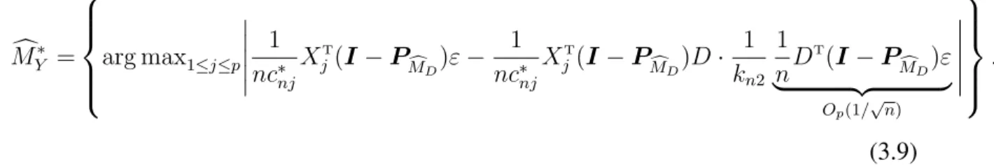
3.5.3 Illustration of (3.9) in Section 3.1.2 . . . 67
3.5.4 Derivation of (3.13) in Section 3.2 . . . 67
3.5.5 Sufficient conditions to control the under-fitting bias . . . 68
3.6 Implementation details . . . 71
4 Average Treatment Effects Estimation . . . 73
4.1 ATE estimation with regression adjustment . . . 73
4.1.1 Notation and setup . . . 73
4.1.2 Simulation study . . . 76
4.2 ATE estimation with doubly robust estimator . . . 77
4.2.1 Doubly robust estimator with repeated data splitting . . . 78
4.2.2 Comparison between R-Split estimator andαeDR . . . 81
4.3 Heterogeneous treatment effects . . . 82
4.4 Proofs . . . 84
4.4.1 Proof of Theorem 3. . . 84
5 Conclusion and Future Work. . . 87
LIST OF FIGURES
Figure
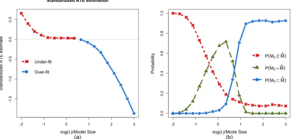
2.1 (a) The left panel shows standardized bias of Alasso+OLS estimator as the tuning parameter λ varies from exp(2) to exp(−3). The horizontal axis is
−log(λ)as a measure of model size. (b) The right panel shows the probabili-ties of under-fittingM0 6⊂Mc, perfect selectionM0 =Mc, and no under-fitting
M0 ⊂Mcin Example 1. . . 11 2.2 Based on 500 Monte Carlo samples. Panel (a)-(b) show the box-plots of|ρb1,n|
and|ρb2,n|for different dimensions. The data generating process is given in the example in Chapter 2.2. . . 13
2.3 Summary for the equal correlation design with Σjk = 0.3and |Mc| = 10as the fraction of the data for model building 1−rv changes from 0.2 to 0.9. The horizontal lines capture the performance of B-Split estimator, which do not change with rv. Panel (a) shows the standardized bias of the smoothed estimator. Panel (b) shows the relative efficiency of the smoothed estimators against the oracle estimator. . . 22
3.1 Based on 1000 Monte Carlo samples, the area of shading lines is the histogram ofρbdouble, and the area with solid blue filling is the histogram ofρbpods. The data generating process is given in Example 3. . . 46
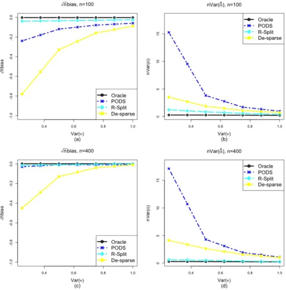
3.2 Finite sample comparison between R-Split and the two-stage selection meth-ods based on Model (3.8). The data generating process is the same as Example 3, except for σ2
ν is a sequence from 0 to 1, and Σjk = 0.9|j−k| is the(j, k)-th element ofΣ, forj, k = 1,· · · , p+ 1. Panels (a) and (c) show the√ntimes the bias of theαestimates. Panels (b) and (d) showntimes the variance of the
αestimates. . . 53
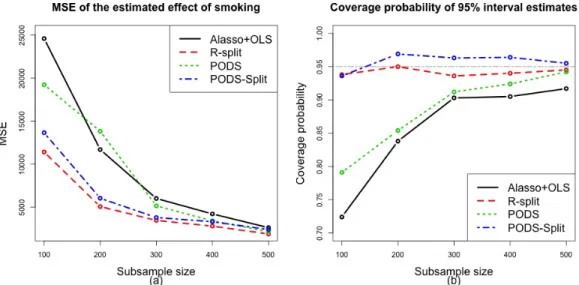
3.3 Finite sample performance for estimating effect of smoking on infants birth weights, aggregated over 1,000 replications. . . 61
3.4 Finite sample performance for estimating effect of smoking on infants birth weights, aggregated over 1,000 replications. The continuous variables are re-placed by their orthogonal polynomial expansions. . . 62
LIST OF TABLES
Table
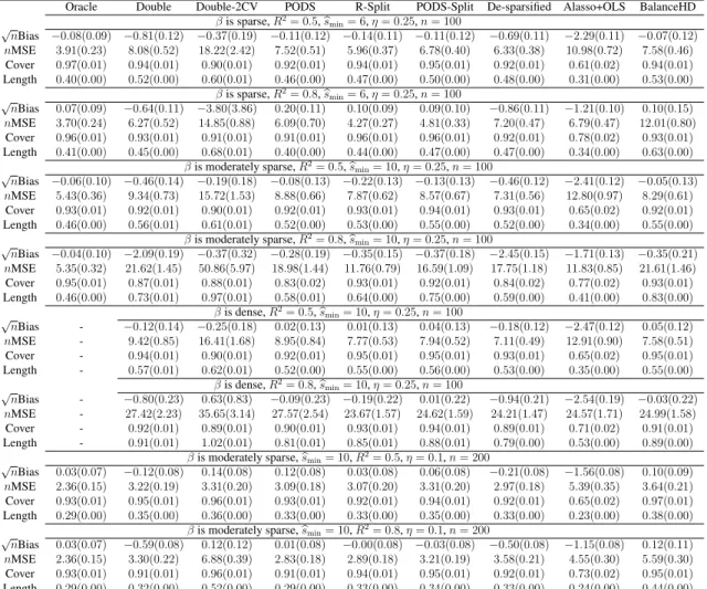
3.1 Performance summaries for various methods under Setting 1 with (n, p) = (100,500). . . 58
3.2 Notations are the same as in Table 3.1. The results are based on Setting 2 with (n, p) = (100,500). . . 59
ABSTRACT
This dissertation concerns the post-selection bias issue in statistical inference on treatment effects when a large number of covariates are present in a linear or par-tially linear model. While the estimation bias in an under-fitted model is well un-derstood, we address a lesser known bias that arises from an over-fitted model. We show that the over-fitting bias can be reduced or eliminated through data splitting, and more importantly, smoothing over random data splits or bootstrap-induced splits can be pursued to mitigate the efficiency loss. We also discuss some of the existing methods for debiased inference and provide insights into their intrinsic bias-variance trade-off, which leads to an improvement in bias controls. Based on these insights, we thoroughly study the connections between our current frame-work and the estimates of the average treatment effects under the Neyman-Rubin causal model. A careful analysis shows that the post-selection bias issue can ex-ist in a wider range of treatment effect estimation procedures. Under appropri-ate conditions we show that our proposed estimators for the treatment effects are asymptotically normal and their variances can be well estimated. We discuss the pros and cons of various methods both theoretically and empirically, and show that the proposed methods are valuable options in post-selection inference.
CHAPTER 1
Introduction
In the modern era, we are often challenged by high dimensional data with many different characteristics per subject. For example, biomedical scientists may study the genomes of patients to choose a precise treatment and to learn the underlying cause of a disease; social scientists study individual behavior from multiple perspectives to decide the effectiveness of a training program. Thus, there is a crucial need to sort through this mass of information in high dimensional data, and provide valid statistical inference. In recent years, two lines of research appear to dominate the literature for high dimensional data analysis.
The first line of research provides statistical inference frameworks for scientists who start their research by running exploratory data analysis on high dimensional data, and form their research questions after model/variable selection. For example, one may assume that the observed data{Yi, Xi}ni=1 are i.i.d and follow a high dimensional linear regression
model
Yi =Xi0β+εi, i= 1,· · · , n,
whereYiis the outcome variable,Xi is the high dimensional covariate,βis a high
dimen-sional sparse vector of coefficients, and ε is a noise variable. In this context, Lee et al.
(2016) and Taylor and Tibshirani (2015) proposed a framework, called “selective infer-ence”, which constructs exact confidence intervals for the selected regression coefficients conditional on the selected model. As long as the selective event can be rewritten as affine constraints on the response vectorY = (Y1,· · · , Yn)0, selective inference forms valid
con-fidence intervals for the selected coefficients. To be more specific, suppose thatM is the set of all variables andMcis the selected set of variables, forj ∈Mc,Lee et al.(2016) finds
the confidence intervalCM
j forβjM with desired coverage probability1−qthat satisfies
P
βjM ∈CjM|Mc=M
= 1−q.
Since the confidence interval is obtained after conditioning on the selection event, it fol-lows that selective inference may produce a conservative inference procedure. Other than selective inference, Berk et al. (2013) and Kuchibhotla et al. (2018) carry out valid post-selection inference (PoSI) by considering all possible model post-selection procedures that could have produced the selected model. As the authors point out, the inferences are also gener-ally conservative but have the advantage that they require neither perfect model selection nor affine constraint on the selection event.
The second line of research is developed for scientists who start with a pre-specified question (e.g., what is the treatment effect of a medical intervention, what is the effect of interest rates on housing price, etc.), and hope to construct confidence intervals to answer that question. In the presence of high dimensional covariates, standard point estimates in the classical theory of statistical inference are usually biased and methodological advances are required. In this thesis, we thoroughly study the bias issue after model selection when the parameter of interest is a fixed quantity, and our analysis is taken to be in the traditional sense of statistical inference.
As there is a growing literature on program evaluations, where estimation of the treat-ment effects is a valuable part of the statistical analysis in analyzing how treattreat-ments or social policies affect the outcome distributions of interest, we focus on the problem of statistical inference on treatment effects in the presence of high dimensional covariates. Suppose that we havenindependent and identically distributed observations from the units indexed by i = 1,· · ·, n. For each unit, let Yi be the outcome andDi be the treatment
variable. In addition, each unit has a vector of features, referred to as potential confounders denoted byWi. We consider the parameter of interestαis in a model of the form
Yi =αDi+g(Wi) +εi, E(εi|Di, Wi) = 0, i=,1· · · , n, (1.1)
where g(·) is an unknown real-valued function and the εi’s are independent random
er-rors. When the dimension of the potential confounders is small relative ton, model (1.1) has been discussed in the literature of treatment effect estimation; see Robinson (1988),
H¨ardle et al.(2012) and, or more recentlyCattaneo et al.(2016). In this thesis, we adopt a framework similar to that ofBelloni et al.(2014). Formally, we assume thatg(Wi)can be
well approximated by a sparse linear combination of the vectorXi =P(Wi) ∈Rp, where P(Wi)is a known transformation ofWi, and then Model (1.1) can be written as
Yi =αDi+XiTβ+Rni+εi, E(εi|Di, Wi) = 0, i= 1,· · · , n, (1.2)
where theRni’s are approximation errors, which will be assumed to be sufficiently small,
andXi is referred to as the covariates in the subsequent analysis.
When the dimension p is greater than n, inference about α cannot be made without regularization or model selection. A major assumption we make in this thesis is the sparsity in β. Formally, we require M0 = supp(β) = {j ∈ {1, . . . , p} : βj 6= 0} has s0 n elements. Without loss of generality, we assume in the theoretical treatment that the response variable and the covariates are all centered so that no intercept is included in the model. In the high dimensional regime, when the approximation errors are small, inference on the treatment effectαis frequently carried out in two ways. One is to perform inference after a sufficiently small model (that includes D) is selected, and the other is to perform debiased inference directly on a regularization method.
In the first chapter of this thesis, we focus on the method where inference is carried out on a selected model. Any reasonable model selection method can be used, for
exam-ple Lasso (Tibshirani,1996), the smoothly clipped absolute deviation penalized maximum likelihood (Fan and Li, 2001), the adaptive Lasso (Zou, 2006) and many others. When perfect model selection is attained, the resulting estimate of the treatment effect achieves the oracle property (Fan and Li,2001), and post selection inference is asymptotically valid, e.g. Minnier et al.(2011). However, perfect model selection often relies on some unrealis-tically strong assumptions, and inference procedures based on the belief of having an oracle estimator may result in substantial biases (Belloni et al., 2014), and see also Example 1 in Chapter 2.
Based on a selected model Mc, a common practice is to refit with the ordinary least
squares (OLS) estimator and then perform inference onα. Since the modelMcis randomly
chosen, there are two possible sources of bias in the OLS estimator. The first is the under-fitting bias when an active covariate is missing in the selected model. To a large extent, the under-fitting bias can be reduced by choosing a larger model that has a high probability of
M0 ⊂ Mc. However, even if the model selection procedure retains all relevant variables,
we demonstrate that the OLS estimator suffers from what we will call “over-fitting bias” when irrelevant variables are selected due to spurious correlation. The over-fitting bias is negligible in low dimensional problems, but becomes evident when p is large. This issue is not as much discussed in the literature but is recognized inHong et al.(2018) and
Chernozhukov et al.(2018) in a related context. An easy solution to avoid this over-fitting bias is the old idea of data splitting.
A main contribution of this thesis is to introduce and examine the method of repeated data splitting, which helps minimize the efficiency loss due to data splitting or cross-estimation. The repeated data splitting approach, which adopts random data splitting or bootstrap-induced data splitting, is similar in spirit to the bagging ofBreiman(1996). For each split, model selection and OLS estimation are performed on two independent parts of the data, and the proposed estimator of α is the average of the estimates over many data splits. Data splitting has been used by other researchers for debiased inference. Wager
and Athey (2017) used data splitting on random forests-based inference on the treatment effect and established the asymptotic normality for the estimator under the assumption that the subsample size with each split does not grow linearly withn, which is different from the splits that we consider for the regression approach. Additionally,Chernozhukov et al.
(2018), Robins et al. (2017) andWager et al. (2016) adopted the approach of data split-ting and aggregation to estimate the treatment effect. A key difference with our work is that these methods use non-overlapping sub-samples for parameter estimation so that the variance of the aggregated estimator is easier to handle, but the splitting-and-aggregation strategy is not pursued to its full potential for variance reduction. We refer this procedure as cross-estimation. As illustrated in our numerical studies, our proposed approach results in better efficiency by allowing repeated data splitting with overlapping sub-samples for estimation. We also note that under stronger parametric assumptions on the noiseε, one may followFithian et al. (2014) to apply the Rao-Blackwell theorem on the data splitting estimator to obtain an optimal estimator that utilizes the full data.
In the second chapter of this thesis, when the parameter of interest α is independent of the selected model, we discuss another line of work for inference that relies on “de-sparsifying” via a two-stage selection procedure, which has been studied in van de Geer
et al. (2014), and Zhang and Zhang (2014) for the high dimensional models. We show
that the de-sparsified Lasso and the post-double-selection method ofBelloni et al.(2014) are asymptotically similar, and they achieve bias reduction by essentially allowing all the covariates, including the inactive ones in Model (1.2), to be used to adjust for the treatment variable first; but these approaches can lead to substantially reduced variability in the post-adjusted treatment variable. Consequentially, there can be significant efficiency loss in the estimation of α as compared to a one-stage selection procedure without adjusting for the treatment variablesD. Our analysis confirms a delicate bias-variance trade-off in the cases where the treatment variable is correlated with some of the covariates that are not active in the model conditional on the treatment.
While the post-double-selection estimator reduces the under-fitting bias, it does not completely avoid the risk of over-fitting. Therefore, building upon the post-double-selection estimator ofBelloni et al.(2014), we discuss a projection-assisted approach to reduce the risks of the under- and over-fitting biases simultaneously. As each method has its own strength, we provide both theoretical and numerical comparisons for those debiased infer-ence methods. When the bias issue is not a main concern, we show that the two-stage selection procedure is not as efficient as the repeated data splitting approach in observa-tional studies.
In the third chapter of this thesis, we consider a special case when D ∈ {0,1} is a binary random variable. Under the Neyman-Ruin causal model and the unconfoundedness assumption, seeNeyman(1923) for detailed discussion, we provide an extension of the re-peated data splitting approach to incorporate propensity score as part of the model, where larger approximation errors can be accommodated as long as the propensity score is well es-timated. For the second part of Chapter 4, we provide a potentially interesting extension of the repeated data splitting approach for estimating heterogeneous treatment effect (HTE). This can be particularly useful to study in subgroup analysis, where the goal often includes reporting treatment effects within subgroups of subjects defined by a variable of interest. For instance, studies in biomedical science may evolve estimating treatment effects for a group of patients at a certain age; studies in marketing often try to estimate the treatment effect for the individuals for whom a job training program may be most beneficial.
The rest of this thesis is structured as follows. In Chapter 2, we use motivating examples to illustrate the bias issue for inference on α by refitting the OLS to a selected model, and we propose the repeated data splitting approach to eliminate the over-fitting bias. In Chapter 3, we discuss the relationship between the de-sparsified Lasso and the post-double-selection, and propose a new projection-assisted approach to further reduce the over-fitting bias in the post-double-selection estimator. We also identify the conditions under which the proposed estimators of the treatment effect are asymptotically normal. In the second part of
Chapter 3, we give theoretical and numerical comparisons for several methods of debiased inference. In the last part of Chapter 3, we illustrate how our proposed methods can be applied to the NCHS Vital Statistics Natality Birth Data to assess the effect of smoking on birth weight. In Chapter 4, we discuss an extension of our framework for estimating the average treatment effect and the heterogeneous treatment effect. Finally, we conclude our work in Chapter 5 with some future directions and discussions.
CHAPTER 2
Bias after Model Selection and Repeated Data
Splitting
In this chapter, we first formalize the notations used in the thesis. Then we discuss the bias issue of the OLS estimator in a selected model, followed by a repeated data splitting approach to remove this bias.
2.1
Notations
Fori = 1,· · · , n, define Zi = (Di, XiT) T ∈ Rp+1, Xi = (Yi, Di, Xi), andX = {Xi}ni=1. Also let Z = (ZT 1,· · · , Z T n), X = (X T 1,· · ·, X T n), D = (D1,· · ·, Dn)T, and Rn =(Rn1,· · · , Rnn)T. SupposeM is a subset of {1,· · · , p}, and for anyp-dimensional
vec-tor a, define aM to be the sub-vector of a indexed by M, and a−M to be the sub-vector
of a indexed by Mc = {1,· · · , p}\M. Let XM = {X·j, j ∈ M}, where X·j is the jth
column ofX, forj = 1,· · · , n, andZM = (D,XM). Let PM = XM(XMTXM)−1XMT,
PM∗ =ZM(ZMTZM)−1ZMT be the projection matrices sending vectors inRnonto the space
spanned byXM andZM, respectively. Also letQM =I−PM, whereI is an-dimensional
identity matrix. Let the index matrixIeM ∈ R(|M|+1)×(p+1) be such thatIeMZi =Zi,M. Let e1 = (1,0,· · ·,0)T, whose dimension is context-specific. Furthermore, letΣ =b ZTZ/n
be the sample covariance matrix, and Σ = E(ZT
i Zi) be the population covariance of the
sub-matrix of the population covariance sub-matrix indexed by setM, i.e.ΣM =E(Zi,MZi,MT ). We
use the notation x .P y to denote x = Op(y). We use to denote the convergence in
distribution. By1T we denote the indicator function of an eventT.
2.2
Over-fitting and under-fitting bias
Based on a properly chosen data-dependent modelMc, the OLS estimator is
(αbOLS,βbOLST )T = arg min{
1 n Xn i=1(Yi−αDi−X T i β)2 :α∈R, β ∈Rp, βMcc = 0}. (2.1) The performance of αbOLS is evaluated by Belloni et al. (2013), which showed that this
estimator has at least the same rate of convergence as Lasso, and has a smaller bias. To heuristically illustrate the impact of the random modelMcon the estimate ofα, we
decom-poseαbOLSas √ n(αbOLS−α) =eT 1 1 nZ T c MZMc −1 1 √ nZ T c Mε | {z } :=bn1(over-fitting) + 1 nD T (I −P c M)D/n −1 1 √ nD T (I−P c M)(Xβ+Rn) | {z } :=bn2(under-fitting) . (2.2)
The first term bn1 labeled “over-fitting” is really due to the correlation between ZMc andε. When Mcis not data-dependent,bn1 has mean zero. Otherwise, we have in general
E(ε|ZMc) 6= 0. In this case the bias of αbOLS as an estimator ofα is in the same order of
1/√n, which would result in biased inference.
If the approximation error Rn is small, the contributor to the“under-fitting” bias, bn2,
vanishes to zero if M0 ⊆ Mc. Wasserman and Roeder(2009), for example, provides
suf-ficient conditions under which P(M0 ⊆ Mc) → 1, as n → ∞, holds for Lasso. Those
in the sense of P(M0 = Mc) → 1 . Therefore, when the estimation efficiency is not a
major concern, selecting a larger model seems to be a simple remedy to avoid the under-fitting bias. Additional methods to reduce the under-under-fitting bias will be discussed in Section 4. Next, we illustrate the over- and under-fitting biases through two examples when β is sparse.
Example 1(A numerical study with the adaptive Lasso). We start with a simple simulation study where the adaptive Lasso is used for variable selection. Implementation details are provided in the Appendix. We refer to this estimator as Alasso+OLS estimator. The data are generated from model(1.2)withRn= 0,α = 3,β = (1,1,0.5,0.5,0· · · ,0)T ∈Rp×1,
and (n, p) = (100,500). We first generate a random matrix Ze ∈ Rn×(p+1) where each row is randomly drawn from N(0,Σ), with Σij = 0.9|i−j|, (1 ≤ i, j ≤ p+ 1). Then let Di = 1(Zei1 >0)andXi,j =Zei,j be the covariates, fori= 1, . . . , n,j = 2, . . . , p+ 1. If a model selection procedure is the oracle, then
P(Mc=M0)→1, σ−1oracle √ n(αbOLS−α) N(0,1), whereσ2 oracle = σε2(Σ −1 M0)11, σ 2
ε = Var(εi), and(Σ−1M0)11 denotes the first diagonal element
ofΣ−1M
0. As the tuning parameterλdecreases fromexp(−3)toexp(−2), we keep track of
the selected modelMcand report the standardized bias ofαOLSb from the selected modelMc. In this setting,αis often refereed to as the average treatment effect (ATE).
The numerical results presented in Figure 2.1 are evaluated though 1000 Monte Carlo samples. From Figure 2.1(a), we see that when λis greater thanexp(1) and some active covariates are often missed in the refitting step, leading to clear under-fitting bias. When the tuning parameter decreases fromexp(2)toexp(1), the under-fitting bias decreases quickly as more covariates are used in the ordinary least squares estimates. However, asλdecreases further to include more and more covariates in the selected model, the bias does not vanish but begins to increase in the opposite direction. By the nature of model selection, the
over-Figure 2.1: (a) The left panel shows standardized bias of Alasso+OLS estimator as the tuning parameter λ varies from exp(2) to exp(−3). The horizontal axis is−log(λ)as a measure of model size. (b) The right panel shows the probabilities of under-fitting M0 6⊂
c
M, perfect selectionM0 =Mc, and no under-fittingM0 ⊂Mcin Example 1.
selected variables are most likely highly correlated with Y in each sample. Since they account for the variability inY in the data, the estimated coefficient onDis attenuated. In this particular example, the over-fitting bias can be as significant as the under-fitting bias, and will lead to invalid statistical inference.
From Figure 2.1(b), we observe clearly that perfect model selection cannot be achieved with high probability, but as λ decreases towards exp(−3), the under-fitting probability decreases rapidly toward 0; and in most of the Monte Carlo samples, the selected model
c
M containsM0. If we use a smallλin the adaptive Lasso, the main issue to be concerned
with is indeed the over-fitting bias for the estimation ofα.
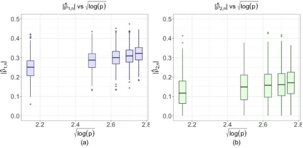
Example 2 (A simple model without covariates). To understand the over-fitting bias, we
consider a simple model to illustrate the point,Y = αD+ε, whereε is the white noise.
For easy notation, suppose our covariates and the response are centered and thus the in-tercept is not considered. The treatment effect is the coefficient ofD. WhenDis a binary random variable, in randomized experiments, this simple model suggests that the treatment assignment is not influenced by any potential confounding factors, both observed and
un-observed. Due to model selection, as we discussed before, we have E(ε|XMc) 6= 0if Mc
contains any covariates fromX.
In this example, the estimated coefficients from the working model with any endoge-nous variables is biased. To simplify the notation, consider the case where only one co-variate (beyond the treatment variable) is included in the working model. In this case, the over-fitting bias can be further simplified into
EαbOLS−α=E b ρ1,nρb2,n−corrdn(ε, D)kDk 2 2/n b ρ2 2,n−1 kεk2 kDk2 ,
where ρb1,n = corrdn(ε,XMc) and ρb2,n = corrdn(D,XMc) are the correlations between the over-selected variable X
c
M and D and ε, respectively. These correlations are similar to
spurious correlations, and may increase in magnitude with p, even when both X and D
are generated completely independent of ε. Fan et al.(2018) addressed a related problem and derived the distribution of the maximum spurious correlation for high dimensional variables.
Next, we provide a simulation study to support the heuristic given above. Letn = 100,
p ∈ {100,500,1000,1500,2000}, α = 1, εi ∼ N(0,1), and generate Zei ∼ N(0,Ip+1),
then letDi = 1(Zi1 >0)andXij =Zeij be the covariates, fori= 1,· · · , n,j = 2,· · · , p+
1. We proceed the model selection step with marginal screening. As the upper bound of over-fitting bias derived in (2.10) increases with √logp, we plot |ρb1,n| and |ρb2,n| against
√
logp. From the results shown in Figure 2.2, we observe that the sizes ofρb1,n, and to a
lesser extentρb2,n, increase with the dimension of the covariates.
Remark 1(Over-fitting bias for predictingY). The over-fitting bias issue we discussed in this section also applies when the goal is to predict the response Y. Consider the refitted
OLS predictionYb =
b
αOLSD+XβOLSb , then even ifM0 ⊆Mc, we have
E(Yb −αD−Xβ) =E Z c M(Z 0 c MZ) −1 Z0 c Mε 6 = 0,
Figure 2.2: Based on 500 Monte Carlo samples. Panel (a)-(b) show the box-plots of|ρb1,n|
and|ρb2,n|for different dimensions. The data generating process is given in the example in
Chapter 2.2.
due to the correlation betweenZ
c
M andε.
2.3
Repeated data splitting
Since the fitting bias is mainly caused by the spurious correlation between the over-selected variables and the noise, it can be easily avoided by the idea of data splitting. Data splitting divides a sample of sizen into two parts: the model building part of sizen1 and
the estimation part of sizen2 = n−n1. The first part of the data is then used for model
selection and the remaining part is used for estimation based on the selected model. Whenβ
is sparse and by selecting a larger model in the first part, we expect the OLS estimator from the second part of the data to be free of significant bias. Rinaldo et al.(2016) considered data splitting for debiased inference. However, it is also clear that data splitting enables debiased inference after model selection at a cost. As only part of the sample can be used in the estimation step, which means a loss of efficiency even if a perfect model has been selected. We consider using repeated splits and then averaging the estimates ofαover those splits. This strategy, similar to bagging or bootstrap aggregating proposed inBreiman
(1996), is a machine learning ensemble meta-algorithm and can help improve the stability and accuracy over a single split or a small number of splits. Similar ideas based on bagging are considered in Meinshausen and B¨uhlmann (2010) andMeinshausen et al. (2009) for the recovery of sparse representations. We consider two data splitting schemes, repeated random splitting (R-Split) and bootstrap-induced splitting (B-Split), in more detail.
2.3.1
R-Split
Based on repeated random data splitting, the estimation and inference procedure for the treatment effectαcan be described as follows (Algorithm 1). First, we setn2 as the upper
bound of the selected model size to ensure the existence of the OLS estimator in any given subsample. Next, the choice of model size is subjective but needs to be large enough for the under-fitting bias to be negligible. In our empirical work, we use Lasso for model selection, and choose the model size from cross-validation with an upper boundn2 minus
a small number to determine the level of penalization; we note that this can be done in standard softwares for regularized regression, such asglmnet.
Algorithm 1R-Split Forb ←1toB do
Step 1. Randomly split the data{(Yi, Di, Xi)}ni=1into groupT1 of sizen1 and
groupT2 of sizen2 =n−n1, and letvbi =1(i∈T2), fori= 1,· · · , n. Step 2. Select a modelMcb to predictY based onT1.
Step 3. Refit the model with the data inT2 to get
(αbb,βbbT) = arg min Pj∈T
2(Yj−αDj −X T
j,Mcb
β)2,
The final “smoothed” estimate isαe= B1 PBb=1αbb.
In Algorithm 1, any reasonable model selection procedures may be used in Step 2. Our empirical studies suggest that the variance of the aggregated estimator is a non-increasing function of B, and the decay slows down if B grows larger than 1,000. Therefore, we recommend usingB = 1,000as a good balance between computational load and statistical inference accuracy. In the theoretical investigations, we considerBto be infinitely large.
Let Vn2 = {V = (V1,· · · , Vn)∈R
n : V
i ∈ {0,1}, Pni=1Vi =n2}be the space of n
-tuples with the l1 norm equalsn2. The data splitting weight vb = (vb1,· · · , vbn) given in
Step 1 takes value in Vn2 with equal probabilityP(V = vb) = 1/
n n2
. For a single split, the selected model can be viewed as a function of the dataX = {Yi, Di, Xi}ni=1 and the
random weightV ∈ Vn2, i.e.Mc=M(X, V). The proposed R-Split estimator can then be defined as the expectation ofαbbgiven the data, that is,αe=E(αbb|X).
Following a strategy proposed inEfron(2014) and the bias corrected version ofWager et al.(2014), we can estimate the variance of the smoothed estimator through the nonpara-metric delta method. The estimated variance takes the following form with the derivation provided in Appendix2.5.6 b σn2 =nXn j=1 n−1 n−n2 b Sj 2 − n2n 2 B2(n−n 2) XB b=1(αbb−αe) 2, (2.3)
whereSbj = B1 PBb=1(vbj − B1 PBk=1vkj)αbb. In Section 3.3, we prove under certain
condi-tions, the smoothed estimatorαeconverges to a normal distribution. We can then construct an approximate(1−q)level confidence interval forαbyαe±Zq/2n−1/2bσn, whereZq/2 is
the1−q/2quantile of the standard normal distribution.
2.3.2
B-Split
In Efron (2014), the author discussed a bootstrap smoothing method to account for the variability of model selection. In that setting, model selection and parameter estimation are performed on the same bootstrap samples, so the over-fitting bias would remain in high dimensional problems. We find that a simple modification to Efron’s approach addresses the bias issue. The proposed method is to draw a bootstrap sample for model selection, and then estimate the treatment effect α using the observations that do not show up in the bootstrap sample. On average, a bootstrap sample takes 0.632n distinct observations from the original sample, even though the bootstrap sample size remains at n. In other
words, we now use the bootstrap-induced splitting, by using the bootstrap sample (of size
n) to perform model selection but choosing observations not used in the bootstrap sample, roughly 36.8% of the original sample, for parameter estimation.
Algorithm 2B-Split Forb ←1toB do
Step 1 Draw a bootstrap sampleX∗b := (X∗
b1,· · ·,X ∗
bn)fromX. Letw
∗
bibe the number of
times theith observationDi appears in the bootstrap sample, and letvbi∗ = 1(w∗
bi=0). Step 2. Select a modelMcb∗ to predictY based onX
∗
b.
Step 3. Refit the selected modelMcb∗ with the observations not in the bootstrap sample
to get(αb∗b,βbbT∗)T = arg minPni=1vbi∗(Yi−αDi−XT i,Mc∗
b
β)2.
The final smoothed estimate isαe= B1 PBb=1αb∗b.
We refer to this bootstrap-induced data splitting as B-Split. Clearly, there is similarity between B-Split and data carving as used in Fithian et al. (2014). Similar to R-Split, we can view the smoothed estimator obtained from Algorithm 2 as a conditional expectation,
e
α = E(αb∗b|X). The weightV∗ = (V1∗,· · ·, Vn∗)is from the setV∗ = {V∗ ∈ Rn : V∗
i =
1(Wi∗=0), i = 1,· · · , n, (W1∗,· · · , Wn∗) ∼Mult(n,1/n)}, where Mult(n,1/n)denotes the
multinomial distribution with n trails and each event has the success probability of 1/n. FollowingEfron(2014) andWager et al.(2014), we can construct a variance estimate for B-Split estimator as b σ2n=nXn j=1Sb ∗2 j − n2 B2 XB b=1(αb ∗ b −αe) 2 , (2.4) whereSbj∗ = 1 B PB b=1(w ∗ bi− 1 B PB k=1w ∗ ki)(αb ∗ b −αe).
2.3.3
Theoretical investigation of R-Split
In this section, we study the theoretical properties of the smoothed estimators. Except for the space of weights V and V∗, B-Split and R-Split are intrinsically the same. To avoid redundancy, we focus on R-Split.
For a fixed modelM and a weightV ∈ Vn2, define the covariance matrix in the given subsample asΣbV,M = n−12
Pn
i=1ViZi,MZ
T
i,M, with the notations thatZi,M = (Di, Xi,MT )
T . Let ZV = (DV,XV)be the design matrix with rows {Zi : Vi = 1, i = 1,· · · , n} and gV(W) = {g(Wi) : Vi = 1, i = 1,· · · , n}. Define the projection matrix in the given
subsample asPV,M =XV,M(XV,MT XV,M)−1XV,MT . Furthermore, letV˘ = ( ˘V1,· · · ,V˘n)∈
Vn2 be from another split independent ofV = (V1,· · · , Vn). SupposeM˘ = M(X,V˘)is the selected model fromV˘, andMc = M(X, V)denotes the selected model fromV, and
let bhi,n= E VieT1Σb−1 V,Mc e I c M X −E VieT1Σb−1˘ V ,M˘IeM˘ X Ziεi, hi,n= E VieT1Σ −1 V,Mc e I c M X −E VieT1Σ −1 ˘ V ,M˘IeM˘ X Ziεi,
where the expectations are taken with respect to V and V˘ conditional on the data. It is helpful to explain the difference between the two expectations in the above definitions. For instance, inbhi,n, note thatV˘ andV have the same distributions, and the first expectation
E VieT1Σb−1 V,Mc e I c M|X =EeT 1Σb−1 V,Mc e I c M|X, Vi = 1 P(Vi = 1),
so the difference of the two expectations in the definition of bhi,n is the difference in the
means due to leaving thei-th observation out for the model selection step in obtainingMc
but not always so in obtaining M˘. With a change of possibly one out ofn observations, the distributions of the quantities involved and their means typically change in the order of
1/nfor most model selection methods. Assumption 3below formalizes this for technical convenience.
Assumption 1. Data generating process. (a). Suppose {(Yi, , Di, Xi)T}ni=1 is a random
sample, and the covariates (Di, Xi) have zero mean and have bounded support with an
error variableεi is sub-Gaussian withE(εi|Zi) = 0andE(ε2i|Zi) =σε2, fori= 1,· · · , n.
Assumption 2. The split ratiorv = n2/nis a constant in(0,1). The selected model sizes
in all split are bounded byswiths=o(n).
Assumption 3. The quantitiesbhi,n’s satisfy Pn
i=1bhi,n/
√
n =op(1).
Assumption 4. There exists a random vector ηn ∈ Rp+1 which is independent of ε, and
||ηn||∞is bounded in probability, and satisfies
rvE eT 1Σb−1 V,Mc e I c M X −ηn 1 =op 1/plogp
Assumption 5. There is negligible amount of under-fitting bias after averaging over all splits in the sense that
E (DT V(I−PV,Mc)DV/n) −1· DT V(I−PV,Mc)gV(W)/ √ n|X=op(1).
Theorem 1 (Asymptotic normality of R-Split estimator). Under Assumptions 1-5, the smoothed estimator from R-Split has the following representation
√ n(αe−α) = ηT n 1 √ n n X i=1 εiZi+op(1). (2.5) Therefore, by lettingeσn=σε ηT nΣbnηn 1/2 , we have e σ−1n √n(αe−α) N(0,1). (2.6) Assumption1requires bounded covariates to simplify our theoretical proofs but it can be relaxed to include sub-Gaussian covariates. Assumption2plays a limit on the sparsity level of the model. This assumption for data splitting is weaker than the ultra-sparsity assumption needed for the post-double-selection or the de-sparsified Lasso. Assumption3
has been discussed following the definitions ofbhi,n and hi,n. Assumption 4says that the
conditional expectation of matrixΣb
−1
c
M for the randomly selected modelMcis asymptotically
independent of the noise, regardless of which point in the sample space is conditioned on. The error rate of1/√logpis a weak requirement for the assumed data generating process. Assumption5is to ensure that the under-fitting bias to be small. Since the selected model size allowed in Assumption 2 can be relatively large, we can choose a larger model than usual to control the under-fitting risk. The proof of the theorem is given in Appendix2.5.2. Sinceηnplays a key role in the asymptotic expression of R-Split estimator, we consider
a special case that Mc = M, where M is a fixed model. In this case, Assumption 3 is
immediately satisfied sincebhi,n = 0, fori= 1,· · · , n. Then,ηnreduces toeT1Σb−1MIeM, and
thus the linear representation in (2.5) simplifies into
√ n(αe−α) =eT 1Σb−1M 1 √ n n X i=1 εiZi,M +op(1).
Therefore, the smoothed estimatorαeshares the same asymptotic expression as theα esti-mate obtained from refitting modelM with the full sample.
To consistently estimate the variance of the smoothed estimator, we adopt the nonpara-metric delta method proposed inEfron(2014). A cleaner version of the linear representa-tion can be provided to build the foundarepresenta-tion of the nonparametric delta method, however, stronger conditions are then required. We make the following assumptions.
Assumption 6. In addition to Assumption2, we haveslogp=o(n).
Assumption 7. The quantitieshi,nsatisfyPni=1hi,n/
√
n =op(1).
Assumption 8. There exists a constant vectorξn ∈ Rp+1 that satisfies||ξn||∞ ≤ C1 for a
constantC1and rvE eT 1Σb −1 V,Mc e I c M X −ξn 1 =op 1/plogp
Assumption 9. The minimums-sparse eigenvalues of the population covariance matrix is positive and bounded away from zero with λmin,s(Σ) ≥ κ0 > 0. There exists a positive
constantK <∞such that,∀V ∈ Vn2,P
lim supn→∞||Σb−1 V,Mc e1||2 ≤K = 1.
Assumption9requires that uniformly over all possible models, thel2-norm of the first
column of inverse of the sample covariance matrix in a subsample of sizen2 is bounded
above from infinity. Under Assumption1and Assumptions6-9, we have
e α=α+ 1 n n X i=1 U(Xi) +op(1/ √ n), (2.7)
whereU(Xi) = εiξTnZi. SinceEU(Xi) = 0andEU(Xi)2 <∞,αeis asymptotically linear
with the influence functionU(Xi). The proof is provided in Appendix2.5.3. Asn → ∞, e
αis asymptotically normally distributed,
σ−1√n(αe−α) N(0,1), (2.8) where σ2 = EU(Xi)2, and σ2 can be consistently estimated by the nonparametric delta
method so thatbσn−σ = op(1), whereσbn is provided in (2.3) for R-Split. Similarly, we
have (2.8) holds for B-Split withbσnprovided in (2.4).
Remark 2(Relationship between the oracle and the smoothed estimators). In R-Split, if perfect model selection is achieved in all splits, the influence functionU(Xi)and the asymp-totic variance reduces toU(Xi) = εieT1Σ
−1 M0Zi,M0 andσ 2 = E{U(Xi)2} = σε2(Σ −1 M0)11.In
this case σ2 equals the asymptotic variance of the oracle estimator, which implies that
under model selection consistency, the smoothed estimator αe achieves oracle efficiency.
However, ifMcb has a positive probability to be a larger model thanM0, e
αis not expected to be oracle.
Remark 3(Comparison between R-Split and cross-estimation). As we mentioned in
cross-estimation for simplicity, supposeV ∈ Vn2 withn2 =n/2, thenαcan be estimated by e αcv = 1 2 ( eT 1 1 n n X i=1 ViZi,Mc1Zi,Mc1 !−1 1 n n X i=1 ViZi,Mc1Yi +eT 1 1 n n X i=1 (1−Vi)Zi,Mc2Zi,Mc2 !−1 1 n n X i=1 (1−Vi)Zi,Mc2Yi ) ,
whereMc1 is the selected model from the subsample indexed by{i:Vi = 0, i= 1,· · · , n}, and Mc2 is selected from subsample indexed by {i : Vi = 1, i = 1,· · · , n}. We show in
Appendix2.5.4that the variance of
e
αcvsatisfies
Var(√n(αcve −α)) =E
Var(√n(αcve −α)|X) +Var(√n(αe−α))≥Var(√n(αe−α)).
(2.9)
Thus, R-Split is more efficient than cross-estimation.
2.4
Finite-sample comparison between R-Split and B-Split
We have the flexibility to choose rv = n2/n in R-Split, where n2 is the number of the
observations used in the estimation. Letω be the variance of the estimated effectαbb from
a single split, andρdenotes the correlation between the estimates of two different random splits. Then the variance of R-Split estimator is of the same order ofρωasB → ∞,
Var(αe) = 1 B2 XB b=1Var(αbb) + 1 B2 X b16=b2 Cov(αbb1,αbb2), = 1 BVar(αb1) + (1− 1 B)Var(αb1)corr(αb1,αb2), →Var(αb1)ρ:=ωρ, asB → ∞.
From this point of view we see the choice of the ratio rv can play a role in Var(αe): by
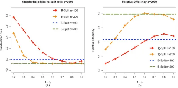
Figure 2.3: Summary for the equal correlation design withΣjk = 0.3and|Mc|= 10as the
fraction of the data for model building1−rvchanges from 0.2 to 0.9. The horizontal lines
capture the performance of B-Split estimator, which do not change withrv. Panel (a) shows
the standardized bias of the smoothed estimator. Panel (b) shows the relative efficiency of the smoothed estimators against the oracle estimator.
which leads to decreased correlation ρ. However, the smaller sample size reduces the accuracy of estimation in each split, which results in larger ω. The optimal choice of rv
at a given sample size is difficult to pin down and it depends on the underlying model. To illustrate this point, we choose B = 2000 in this subsection so that ωρ provides a more accurate approximation of Var(αe).
Consider the same data generating process in Example 1 except for we set Σjk =
0.31(j6=k), (n, p) = (100,2000) or (200,2000), and β = (1,1,1,1,0,· · · ,0)T
. We use Lasso for model selection, is implemented with R packageglmnet. Furthermore, in each split, we select a model from the Lasso path whose model size is the closest to s = 10, a model size that keeps the under-fitting risk at a negligible level with strong signals. We report two quantities through simulation: (a) the ratio of the bias of R/B-Split estimator rel-ative to the standard deviation of the oracle estimator, (b) the asymptotic relrel-ative efficiency of R/B-Split estimator to the oracle estimator.
summa-rize the results in two points. From Figure 2.3(a), B-Split tends to have small bias and so does R-Split withrv below 0.4. From Figure 2.3(b), the smoothed estimators from B-Split
and R-Split withrv ≈ 0.4are nearly as efficient as the oracle atn = 200 but the relative
efficiency is never above 0.7 at n = 100. In this model, B-Split does well, and R-Split with at least 60% of the data in the model selection stage does almost as well in terms of both bias and variance. For smaller n (say n = 100), the under-fitting bias would be an issue ifn1, the subsample size for model selection is small. Then, R-Split benefits from
the flexibility of choosingrv to be small, that is, R-Split can outperform B-Split in such
cases. For largern, B-split is usually a solid choice in this case and many other cases that we have considered. The impact of the choice ofrv in R-Split is expected to diminish as nincreases. Since R-Split and B-Split have similar performances wheneverrv ∈[0.6,0.7],
in the following subsections, we focus on the performance of R-Split withrv = 0.7.
2.5
Proofs
2.5.1
Useful lemmas
In this section, we prove two useful lemmas that shall be used in the later proofs.
Lemma 1. Under Assumption 1,kZTε/√nk
∞=Op(
√
logp).
Proof: Letδj = (Pni=1Zij2)1/2andUij =εiZij/δj. ForK >0, we have
P max j n X i=1 Zijεi/ √ n > p logpK ! ≤E ( P max j δj ·maxj n X i=1 Uij/ √ n > p logpK Z !) ≤pE ( P n X i=1 Uij/ √ n > p logpK/max j δj Z !) ≤2 exp logp− logpK 2 2σ2 εC2 ,
and the right hand side converges to zero whenK is sufficiently large.
As an application of this Lemma, we can provide an upper bound of the over-fitting bias. Following the derivation of the bias decomposition in (2.2), and under the assumption that there exists a positive constantλ0 such that
P lim n→∞λ −1 s,min 1 nZ T Z≥λ0 = 1, we have bn1 =eT1 1 nZ T c MZMc −1 1 √ nZ T c Mε ≤ke1k2λ−1min 1 nZ T c MZMc k√1 nZ T c Mεk2 ≤λ−1min 1 nZ T c MZMc |Mc|1/2· kZTε/ √ nk∞ =Op |Mc|1/2 p logp. (2.10)
Lemma 2. Under Assumptions 1 and 13 , we have
max |M|≤s DT(I−PM)D/n−(Σ11−ΣTD,MΣ−1MΣD,M) =op(1), wherePM =XM(XMTXM)−1XMT. Proof: DenotekAk={tr(AAT)}1/2
for an arbitrary matrixA. To obtain the result, we prove the following two uniform convergence results hold:
max |M|≤skn −1 DT XM −ΣD,Mk=op(1), (2.11) max |M|≤s kn−1XT MXM −ΣMk=op(1). (2.12)
In (2.11), letPni=1DiXij/n =σbD,j andΣD,M = (σD,j, j ∈M)∈R |M| , we have kn−1DT XM −ΣD,Mk= X j∈M (bσD,j−σD,j)2 1/2 ≤s1/2max j∈M |bσD,j −σD,j|,
when|M| ≤s. Therefore,∀ >0by adopting similar arguments used in Lemma1
P max |M|≤skn −1 DT XM −ΣD,Mk> ≤ X |M|≤s X j∈M P |bσD,j −σD,j|> s −1/2 ≤sps2 exp − n 2 2C2s = exp slogp+ logs− n 2 2C2s . (2.13)
By Assumption 13, the right hand of (2.13) converges toward 0 as n → ∞. Applying similar techniques to those used in (2.11), we can also demonstrate (2.12). As a minor generalization of this lemma, we have
P max j |maxM|≤s kZT jZM/n−Σj,Mk2 > ≤exp
logp+slogp+ logs− n 2
2C2s
=o(1).
Similarly, since the covariates are bounded by same constantC andn2/n=rv is bounded
away from 0 and 1, we have for a random subsampleV,
P max j |maxM|≤skZ T j,VZV,M/n2−Σj,Mk2 > ≤E P max j |maxM|≤skZ T j,VZV,M/n2 −Σj,Mk2 > |V ≤exp
logp+slogp+ logs− rvn 2
2C2s
=o(1).
2.5.2
Proof of Theorem 1 in Section
2.3.3
In this part, we provide the proof of Theorem 1.
Step 1. The estimated treatment effect based on model M through ordinary least squares by using full sample can be written as
b αM =eT1(Z T MZM)−1ZMTY =α+eT 1(Z T MZM)−1ZMTε+e T 1(Z T MZM)−1ZMT(Xβ+Rn) =α+eT 1(Z T MZM)−1IeMZTε+ (DT(I −PM)D)−1DT(I−PM)(Xβ+Rn), (2.14)
wheree1 = (1,0,· · ·,0)T ∈Rp+1, andPM = XM(XMTXM)−1XMT. Since the
decompo-sition given above is very important to understand the bias issue after model selection, we provide a detailed derivation for the last equality. By block matrix inversion, the first row of matrix(ZT MZM)−1 equals (DT (I−PM)D)−1,−(DT(I −PM)D)−1DTXM(XMTXM)−1 ,
and then multiply this quantity byZT
M = (D T,XT M), we get eT 1(Z T MZM)−1ZMT = (D T (I−PM)D)−1,−(DT(I −PM)D)−1DTXM(XMTXM)−1 (DT ,XT M) = (DT (I −PM)D)−1DT−(DT(I−PM)D)−1DTXM(XMTXM)−1XMT = (DT (I −PM)D)−1DT−(DT(I−PM)D)−1DTPM = (DT (I −PM)D)−1DT(I −PM). (2.15) Therefore, we obtain eT 1(Z T MZM)−1ZMT(Xβ+Rn) = (DT(I−PM)D)−1DT(I −PM)(Xβ+Rn).
(2.2) in Section 2.2: √ n(αbOLS−α) =eT1 1 nZ T c MZMc −1 1 √ nZ T c Mε + 1 nD T (I−PM)D −1 1 √ nD T (I−P c M)(Xβ+Rn).
Step 2.Now suppose we take a subsample of sizen2indexed by weightV = (V1,· · · , Vn),
let ZV = (DV, XV) be the design matrix with rows {Zi : Vi = 1, i = 1,· · · , n} and gV(W) = {g(Wi) : Vi = 1, i = 1,· · · , n}. Denote the covariance matrix and the
projec-tion matrix in this subsample asΣbV,M =ZV,MT ZV,M/n, andPV,M =XV,M(XV,MT XV,M)−1XV,MT
respectively. LetX ={(Yi, Zi)}ni=1. Consider the smoothed estimatorαe:
√ n(αe−α) =E √n(αbMc−α0)|X =√1 n n X i=1 E eT 1Σb−1 V,Mc e IMcVi X Ziεi +E√n(DT V(I−PV,Mc)DV) −1 DT V(I −PV,Mc)gV(W)|X =√1 n n X i=1 ηT nZiεi+rn1+rn2, where rn1 = 1 √ n n X i=1 E eT 1Σb −1 V,Mc e I c MVi X −ηn Ziεi, rn2 =E √ n(DT V(I−PV,Mc)DV) −1 DT V(I−PV,Mc)XVβ|X .
Step 3. (Behavior ofrn1.) Inrn1, by conditioning onVi = 1 E eT 1Σb−1 V,Mc e I c MVi X =E eT 1Σb−1 V,Mc e I c MVi X, Vi = 1 P(Vi = 1|X) =rvE eT 1Σb−1 V,Mc e I c M X, Vi = 1 . The termE eT 1Σb−1 V,Mc e I c M X, Vi = 1 is the average ofeT 1Σb−1 V,Mc e I c
M over all possible models
but excluding theith point. Let Ve = (Ve1,· · · ,Ven)be another set of splitting weight that
is independent withV, and denoteMfas the selected model indexed byVe. Following the
definition in Assumption 3, the remainder termrn1 can be decomposed into two parts
rn1 = rvE eT 1Σb −1 e V ,Mf e I f M X −ηn T 1 √ n n X i=1 Ziεi | {z } ra n1 +√1 n n X i=1 E eT 1Σb−1 V,Mc e I c MVi X −E eT 1Σb−1 f M ,Ve e I f MVi X T Ziεi | {z } rb n1 . By Assumption 3,rbn1 =Pni=1hi,n/ √
n =op(1). Next, by H¨older’s inequality, Assumption
4 and Lemma1, we have
rna1 ≤rvE eT1Σb−1 e V ,Mf e I f M X −ηn 1· kZ T ε/√nk∞=op(1). Therefore,rn1 =op(1).
Step 4. (Behavior ofrn2.) rn2 captures the under-fitting bias, and is small by
Assump-tion 5: rn2 =E (DT V(I−PV,Mc)DV/n) −1· DT V(I −PV,Mc)gV(W)/ √ n|X=op(1).
Finally, the results in Steps 3 and 4 imply √ n(αe−α) = ηT n 1 √ n n X i=1 εiZi+op(1).
2.5.3
Derivation of
(
2.7
)
in Section
2.3.3
In this part, we provide the derivation of expression that includes the influence functions in (2.7) is provided in2.5.3. Following similar idea to the proof of Theorem 1, by direct calculation √ n(αe−α) =E √n(αb c M −α0)|X =√1 nξ T n n X i=1 Ziεi+tn1+tn2+rn2, where tn1 = 1 √ n E eT 1Σ −1 c MIeMcVi X −ξn T n X i=1 Ziεi, tn2 = 1 √ n n X i=1 E eT 1Σb−1 V,Mc e IMc−eT 1Σ −1 c MIeMc T ViZiεi X .
In this expression, tn1 can be bounded following similar steps in Section B.1 under
As-sumptions7and8. Intn2, letB =
n n2 −1 and we have tn2 = B X b=1 P(V =vb) eT 1Σb−1 vb,Mcb −eT 1Σ −1 c Mb T 1 n n X i=1 vibεiZi,Mcb =1 B B X b=1 eT 1Σb−1 vb,Mcb −eT 1Σ −1 c Mb T 1 n n X i=1 vibεiZi,Mcb =: 1 B B X b=1 tn,vb.
Denote by T1,b the subsample for model building, and T2,b the subsample for parameter
estimation. Defineµi,b =eT1(Σb−1 vb,Mcb −Σ−1 c Mb )Zi, c
thentn,vb satisfies tn,vb = eT 1Σb−1 vb,Mcb −eT 1Σ −1 c Mb T 1 √ n n X i=1 vibεiZi,Mcb = √ n n2 X i∈T2,b εiµi,b := √ nubσε 1 n2 X i∈T2,b µ2i,b 1/2 , where ub = X i∈T2,b µ2i,b −1/2 X i∈T2,b εiµi,b.
We note that{u1,· · · , uB}are dependent but identically distributed random variables. The
variance oftn,vb then equals
Var(tn,vb) =E(Var(tn,vb)|µi,b) +Var(E(tn,vb)|µi,b) =
nσ2 ε n2 E 1 n2 X i∈T2,b µ2i,b.
Next, we provide an upper bound forP i∈T2,bµ
2
i,b/n2. Note that
1 n2 X i∈T2,b µ2i,b =eT 1 b Σ−1 vb,Mcb −Σ−1 c Mb 1 n2 X i∈T2,b Zi, c MbZ T i,Mcb b Σ−1 vb,Mcb −Σ−1 c Mb e1 =eT 1Σb−1 vb,Mcb b Σv b,Mcb−ΣMcb Σ−1 c Mb b Σv b,Mcb −ΣMcb b Σ−1 vb,Mcb e1 ≤λmax Σ−1 c Mb e T 1Σb−1 vb,Mcb b Σv b,Mcb −ΣMcb 2 2 ≤ λ−1minΣ c Mb e T 1Σb−1 vb,Mcb 2 2 λ2maxΣbv b,Mcb−ΣMcb ≤K2/κ0λ2max b Σv b,Mcb−ΣMcb ,
where the last step is obtained by Assumption 9. Since the covariates are bounded by
C, by applying Corollary 5.50 in Vershynin (2016), we obtain that under Assumption 6
and the fact that Mcb is selected independent with Σbvb, P{λmax(Σbv
2 exp(−nε2/C).Therefore for all possible models, P h λmax b Σv b,Mcb−ΣMcb ≥for anyMcb i ≤2 exp slogp− n 2 C , (2.16)
by Assumption6, and the above upper bound converges to 0 as n → ∞. Therefore with probability tending to 1, for all >0and for allvb ∈ Vn2,n
−1 2 P i∈T2,bµ 2 i,bis bounded by. By lettingH n ={for allvb ∈ Vn2, n −1 2 P i∈T2,bµ 2 i,b ≤}, we haveP(Hn)→1asn → ∞. For any0 >0, P(tn2 > 0) =Pn1 B XB b=1ubσεn −1 2 X i∈T2,b µ2i,b 1/2 > n−1/20 o ≤Pnσε 1 B XB b=1u 2 b 1/21 B XB b=1 1 n2 X i∈T2,b µ2i,b 1/2 > n−1/2n12/20 o ≤Pnσε 1 B XB b=1u 2 b 1/21 B XB b=1 1 n2 X i∈T2,b µ2i,b 1/2 > n−1/2n12/20 H n o P(Hn) +P(H ,c n ) ≤Pnσε 1 B XB b=1u 2 b 1/2 > n−1/2n12/20 o P(Hn) +P(H ,c n ) ≤ 2σ2 εvar n 1 B PB b=1u2b 1/2o n−1n 220 P(Hn) +P(H ,c n ) =O(2−20 )P(Hn) +P(Hn,c).
Therefore, by lettinggo to zero, we havetn2 =op(1). This completes the proof.
2.5.4
Derivation of
(
2.9
)
in Section
2.3.3
In this subsection, we provide the derivation of the comparison between cross-estimation and R-Split is provided in2.5.4. SinceV andVc = {1−V
1,· · · ,1−Vn}are identically
distributed random vectors, then
E( √ n(αecv−α)|X) = √ nE eT 1 1 n n X i=1 ViZi,Mc1Zi,Mc1 !−1 1 n n X i=1 ViZi,Mc1εi X =√n(αe−α).
Thus Var{E(√n(αecv−α)|X)}=Var(√n(αe−α)), and Var(√n(αecv−α)) = E Var(√n(αecv−α)|X) +Var E( √ n(αecv−α)|X) =E Var(√n(αecv−α)|X) +Var( √ n(αe−α))+≥Var(√n(αe−α)).
2.5.5
Derivation of
(
3.12
)
in Section
3.2
In this part, we provide the proof of the alternative expression for the variance of R-Split that has been shown in Section2.5.5. Recall the additional assumptions we made in Section 5.
Assumption 10. On average, the maximum “correlation” between D and X after con-trolling for the effects inX
c
M is bounded above by
√
logpin probability, or more formally, E ( DT V(I −PM ,Vc )XV/n DT V(I −PM ,Vc )DV/n X ) ∞ =Op( p logp). (2.17)
Assumption 11. The maximals−sparse eigenvalue satisfiesP(lim supn→∞λmax,s(XTX/n)≤ K0) = 1. The maximum eigenvalue ofΣb is bounded bylogpin probability.
We start with generalizing the result stated in (2.16). For all possible models,
P n λmax b ΣV, c MV −Σbn,McV ≥o (2.18) ≤Pnλmax b ΣV, c MV −ΣMcV ≥/2o+Pnλmax b Σn, c MV −ΣMcV ≥/2o ≤E Pnλmax b ΣV,Mc V −ΣMcV ≥/2|Vo+E Pnλmax b Σn,Mc V −ΣMcV ≥/2|Vo ≤4 exp slogp− n2 2 C = 4 exp slogp− rvn 2 C =o(1). Letηbn = rvE eT 1Σb−1 V,Mc I c M|X T , by Assumption4, we have||ηn−ηbn||1 = op(1/ √ logp).
We next prove the followings ηT nΣbnηn= b ηT nΣbn b ηn+op(1), (2.19) b ηT nΣbnηbn≤r 2 vE eT 1Σb −1 V,Mc b Σ c MΣb −1 V,Mc e1|X =ErveT1Σb −1 V,Mc e1|X +op(1). (2.20)
With (2.19) and (2.20), if we further assume the selected model size satisfies ultra-sparsity in the sense that|Mc|logp/
√ n=o(1), we obtain E rveT1Σb −1 V,Mc e1|X =E (Σ−1 c M)11 X +op(1)
by Lemma 2 under Assumptions1,4and13. Therefore, we haveσen2 ≤σ2εE (Σ−1 c M)11 X +
op(1). We next prove (2.19) in step 1 and prove (2.20) in step 2.
Step 1. In (2.19), by Assumptions11and4,
ηT nΣbnηn−ηbnTΣbnbηn = (ηn−ηbn)TΣbn(ηn−bηn) + 2(ηn−bηn)TΣbnbηn ≤λmax(Σbn)||ηn− b ηn||21+||ηn−bηn||1||Σbnηbn||∞ =op(1) +||ηn−bηn||1||Σbnηbn||∞,
In the second part,
b Σnηbn =rvE b ΣnIT c MΣb −1 V,Mc e1|X =E 1 n n X i=1 ZiZi,TMc− 1 n2 n X i=1 ViZiZi,TMc ! 1 n2 n X i=1 ViZi,McZ T i,Mc !−1 e1 X +E 1 n2 n X i=1 ViZiZi,T c M ! 1 n2 n X i=1 ViZi,McZ T i,Mc !−1 X :=qna1+qnb1,
whereqb
n1can be further simplified
qnb1 =E ( DT V(I −PM ,Vc )XV DT V(I −PM ,Vc )DV X ) , and satisfies qnb1 ∞=Op( √ logp)by Assumption3.11. Inqa n1, ||qan1||∞ =E 1 n n X i=1 ZiZi,TMc− 1 n2 n X i=1 ViZiZi,TMc ! 1 n2 n X i=1 ViZi,McZ T i,Mc !−1 e1 X ≤rvE ||Σb−1 V,Mc e1||2max j ||Z T jZMc/n−Σj,Mc||2 X +rvE ||Σb−1 V,Mc e1||2max j ||Z T j,VZV,Mc/n2−Σj,Mc||2 X .P rvK·max j |maxM|≤s||Z T jZM/n−Σj,M||2 +rvKE max j |maxM|≤s ||ZT j,VZV,M/n2−Σj,M||2 X .P op(1) +rvKE max j |maxM|≤s ||ZT j,VZV,M/n2−Σj,M||2 X ,
where the last inequality is obtained by Lemma 2. Define an event
E max j |maxM|≤s||Z T j,VZV,M/n2−Σj,M||2 =E max j |maxM|≤s||Z T j,VZV,M/n2−Σj,M||2 Ln P(Ln) +E max j |maxM|≤s||Z T j,VZV,M/n2−Σj,M||2 L,cn P(L,cn ) ≤s1/2(C+||Σ||∞) exp
logp+slogp+ logs− rvn 2
2C2s
+=o(1);
by letting go to zero, then we get ||qa
n1||∞ = op(1). This completes the proof of
Step 2. For the first part of (2.20), we have b ηT nΣbn b ηn =rv2E eT 1Σb−1 V,Mc e I c M|X 1 nZ T ZEIeT c MΣb −1 V,Mc e1|X =rv2EeT 1Σb −1 V,Mc ZT c M/ √ n|XEZ c MΣb −1 V,Mc e1/ √ n|X ≤rv2EeT 1Σb−1 V,Mc b Σ c MΣb −1 V,Mc e1|X .
Next we prove the difference betweenr2vEeT
1Σb−1 V,Mc b Σ−1 c MΣb −1 V,Mc e1|X andErveT1Σb−1 V,Mc e1|X is negligible. Consider r2vEeT 1Σb−1 V,Mc b Σ c MΣb −1 V,Mc e1|X −ErveT1Σb−1 V,Mc e1|X =r2vEeT 1Σb−1 V,Mc b Σ c MΣb −1 V,Mc e1|X −ErveT1Σb−1 V,Mc b ΣV, c MΣb −1 V,Mc e1|X =r2vE eT 1Σb−1 V,Mc b Σ c M − 1 rv b ΣV, c M b Σ−1 V,Mc e1|X =r2vE ( eT 1Σb−1 V,Mc 1 n n X i=1 Zi, c MZ T i,Mc− 1 n2 n X i=1 ViZi,McZ T i,Mc ! b Σ−1 V,Mc e1|X ) ≤r2vE ( λmax 1 n n X i=1 Zi,McZT i,Mc− 1 n2 n X i=1 ViZi,McZ T i,Mc ! ||Σb−1 V,Mc e1||22|X ) ≤r2vE ( λmax 1 n n X i=1 Zi,McZT i,Mc− 1 n2 n X i=1 ViZi,McZ T i,Mc ! K2|X ) By letting G n = n λmax 1 n Pn i=1Zi,McVZ T i,McV − 1 n2 Pn i=1ViZi,McVZ T i,McV K2 ≤o, by (2.18), we haveP(G
n)→1asn → ∞. Therefore, since the maximum
eigenval-ues are bounded above, we obtainr2vEeT
1Σb−1 V,Mc b ΣMcΣb−1 V,Mc e1|X −ErveT1Σb−1 V,Mc e1|X = op(1), which is (2.20).
2.5.6
Derivation of variance estimation in R-Split via the non-parametric
delta method in Section
2.3.1
Recallvb = (vb1,· · · , vbn)is the data splitting weights in thebth split: ifvbi= 1, data point
Xiis used in the refitting step.vbtakes value from sample spaceVn2, wheren2 =
Pn i=1vbi
denotes the total number of samples used for refitting, and
Vn2 = n V = (V1,· · ·, Vn)∈Rn : Vi ∈ {0,1}, Xn i=1Vi =n2 o . LetB = nn 2
and there areB components inVn2. Since all the weights are independently generated, we have pr(V =vb) = 1/B,forb= 1, . . . , B.Following the definition inEfron
(2014), the ideal smoothed estimation isαe=PBb=1P(V = vb)αbb,and it can be viewed as
a functional of the empirical distributionFbn, denotes asT(Fbn). When adding a point mass δXjat directionj,j ∈ {1, . . . , n}, the empirical distributionFbnchanges to(1−)Fbn+δXj, and the influence function can be written as
U(Xj,Fbn) = lim →0
T((1−)Fbn+δXj)−T(Fbn)
. (2.21)
Data splitting takesn2subsamples without replacement and without regard to the order.
The subsamples can be viewed as taken all at once from the entire population ofnobjects, while each sample shares the same probability being chosen. Thus, the average number of a given sampleXj in the subsampleE(#ofXj in the subsamples of sizen2) = n2/n.
If a point massδXj is added inFbn, this means the probability ofXj increases from1/n to(1−)/n+, and the probability of the other objects decreases from1/nto(1−)/n. We denote the perturbed empirical distribution function asFbnj. After the perturbation,
E(#ofXj in the subsamples of sizen2) (2.22)
=n2 1− n + =P
Xj being selected in the subsamples of sizen2underFbnj
Define a subset Bj = {vb : vb ∈ Vn2andvbj = 1} ⊂ Vn2, which indexes the entire possible combinations that includeXj. The cardinality of the subsetBj equals to
n−1 n2−1 = Bn2 n . (2.23)
After the perturbation on thejth direction, inVn2, only the elements withVj = 1share the same probability of being chosen. This givesP(V =vb1,Xj being chosen underFb
j n) =
P(V =vb2,Xj being chosen underFb
j
n),for allb1, b2 ∈ Bj,and X
b∈BjP
(V =vb,Xj being chosen underFbnj) =P(Xj being chosen underFbnj). (2.24)
From (2.22)–(2.24), we have
P(V =vb,Xj being chosen underFbnj) = n2{(1−)/n+}/{Bn2/n},
and similarlyP(V =vb,Xj not being chosen underFbnj) ={1−n2{(1−)/n+}}/{B− Bn2/n}.Hence, after adding a small perturbation onjth direction,
P(V =vbunderFbnj) =vbjP(V =vb,Xj being chosen underFbnj)
+ (1−vbj)P(V =vb,Xj not being chosen underFbnj)
=vbj n2 1−n+ Bn2/n + (1−vbj) 1−n2 1−n + B−Bn2/n =B−1 1 +n(n−1) n−n2 (vbj− n2 n ) .
Using (2.21), U(Xj,Fbn) = lim →0 −1{ T((1−)Fbn+δXj)−T(Fbn)} = lim →0 −1XB b=1 n P(V =vb underFbnj)−P(V =vbunderFbn) o b αb =n(n−1) n−n2 1 B B X b=1 vbj− n2 n b αb =n(n−1) n−n2 cov(α, Vb j).
The nonparametric delta method suggests the standard deviation of the smoothed estimator to be estimated by n−1Xn j=1U 2(X j,Fbn) =n Xn j=1 n n−1 n−n2 b Sj(V,X) o2 (2.25)
where the covariance can be estimated by the data splitting samples
b Sj(V,X) =B−1 XB b=1(vbj−B −1XB k=1vkj)αbb. (2.26)
In practice, the smoothed estimator are computed using a finite numberB of the data split-ting, and working with a large B can be computationally expensive. Without sufficient number of splitting, the formula in (2.26) is biased upward argued inWager et al.(2014). Following similar method as in Wager et al.(2014), the Monte Carlo bias in M-Split can be corrected and the variance can be estimated through equation (2.3).