Performance, Power Modeling and Optimization for
High-Performance Computing Systems
A DISSERTATION
SUBMITTED TO THE FACULTY OF THE GRADUATE SCHOOL OF THE UNIVERSITY OF MINNESOTA
BY
Chi Xu
IN PARTIAL FULFILLMENT OF THE REQUIREMENTS FOR THE DEGREE OF
Doctor of Philosophy
John Sartori
© Chi Xu 2016 ALL RIGHTS RESERVED
Acknowledgements
There are many people that have earned my gratitude for their contribution to my time in graduate school.
I wish to thank my committee members who were more than generous with their expertise and precious time. A special thanks to Dr. John Sartori, my advisor for his countless hours of reflecting, reading, encouraging, and most of all patience throughout the entire process.
I would like to acknowledge and thank my school division for allowing me to conduct my research and providing any assistance requested. Special thanks goes to the members of staff development and human resources department for their continued support.
Finally I would like to thank the beginning teachers, mentor-teachers and admin-istrators in our school division that assisted me with this project. Their excitement and willingness to provide feedback made the completion of this research an enjoyable experience.
Dedication
I dedicate my dissertation work to my family and many friends. A special feeling of gratitude to my loving parents, Xinzhi Xu and Yingjie Zhao whose words of encourage-ment and push for tenacity ring in my ears. My cousin Fan Xu, who has never left my side and is very special.
I also dedicate this dissertation to my many friends who have supported me through-out the process. I will always appreciate all they have done, especially during those hard times in my school life.
Abstract
Heterogeneity abounds in modern high-performance computing systems. Applications are heterogeneous, containing time-varying unbalanced utilization for different resources, and system architectures have become heterogeneous in order to achieve higher levels of performance and energy efficiency. The most powerful, and also the most energy-efficient high-performance computing systems today consist of many-core CPUs and GPGPUs with a variety of specialize on-chip and off-chip memories. These heterogeneous sys-tems provide a huge amount of computing resources, but it is becoming increasingly challenging to use them effectively and efficiently to maximize their potential. This becomes an even more pressing challenge as energy efficiency becomes the primary bar-rier to achieving higher levels of performance. This thesis addresses the challenges of performance modeling and optimization in heterogeneous high-performance computing systems. Effective system optimization requires understanding of how performance and power change in response to optimizations. Therefore, we begin by summarizing the impact of modern architectural advances on performance and power modeling for chip multiprocessors (CMPs). We present two models that estimate the performance and power in such systems. The first model, CAMP, is a fast and accurate cache-aware per-formance model that estimates the perper-formance degradation due to cache contention of processes running on cache-sharing cores. We then propose a system-level power model for a multi-programmed CMP environment that accounts for cache contention. We explain how to integrate the two models to enable power-aware process assignment. Then, we propose an off-chip memory access-aware runtime DVFS control technique that minimizes energy consumption subject to a constraint on application execution time.
The second part of the dissertation focuses on improving performance for GPGPUs. After a thorough analysis on CPI breakdown, we lay out all the key factors that govern GPU throughput. In order to improve overall performance for GPGPUs, we propose two approaches that address the key factors, without introducing extra congestion and degradation to the system. We first propose a new two-level priority scheduling policy to improve overall performance by optimizing effective degree of parallelism. Then,
including architectural support and a contention-aware workload scheduling algorithm that improves all the key factors in a balanced fashion. Furthermore, we propose a new contention-aware analytical performance model that provides fine-grained workload scheduling decisions for intra-core multitasking, including detailed resource allocation from co-scheduled workloads.
Contents
Acknowledgements i Dedication ii Abstract iii List of Tables x List of Figures xi 1 Introduction 11.1 Modeling High-Performance Computing Systems . . . 2
1.2 Optimizing High-Performance Computing Systems . . . 4
1.3 Scheduling High-Performance Computing Systems . . . 5
1.4 Dissertation Overview . . . 5
2 Multi-core CPU Overview 7 2.1 Introduction . . . 7 2.2 Background . . . 8 2.3 Motivation . . . 8 3 Performance modeling on CMPs 10 3.1 Introduction . . . 11 3.2 Related Work . . . 12 3.3 Analytical Model . . . 13 3.3.1 Background . . . 14 v
3.3.3 Performance Model . . . 16
3.3.4 Estimating Effective Cache Size AfternAccesses . . . 17
3.3.5 Steady-State Conditions . . . 18
3.4 Automated Profiling . . . 19
3.4.1 Reuse Distance Profiling . . . 20
3.4.2 Automated Parameter Estimation . . . 22
3.4.3 Potential Sources of Error . . . 23
3.5 Evaluation Methodology and Results . . . 24
3.5.1 Experimental Setup . . . 24
3.5.2 Pre-Characterization . . . 25
3.5.3 Model Validation . . . 27
3.5.4 Generality of Predictor For Different Machines . . . 31
3.6 Conclusion . . . 32
4 Power Modeling for CMPs 33 4.1 Introduction and Motivation . . . 34
4.2 Related Work . . . 35
4.3 Power Modeling . . . 35
4.3.1 Problem Formulation . . . 36
4.3.2 Handling Context Switching and Cache Contention . . . 37
4.4 Combining Performance and Power Models . . . 38
4.5 Experimental Results . . . 40
4.5.1 Experimental Setup . . . 41
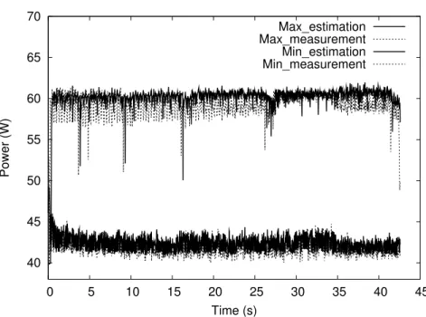
4.5.2 Power Model Validation . . . 41
4.5.3 Combined Model Validation . . . 43
4.6 Conclusions . . . 44
5 Memory access aware on-line voltage control for performance and en-ergy optimization 45 5.1 Introduction and Related Work . . . 46
5.2 Motivation and Problem Formulation . . . 49
5.2.1 Trade-offs Between Performance and Energy . . . 49
5.3 System Modeling . . . 51
5.3.1 Performance Modeling . . . 52
5.3.2 Power Modeling . . . 53
5.3.3 Cost Minimization . . . 54
5.3.4 System Architecture for P-DVFS . . . 61
5.4 Experimental Results . . . 62
5.4.1 Experimental Setup . . . 62
5.4.2 Comparison with Prior Work . . . 63
5.4.3 Experimental Results . . . 64
5.5 Conclusions . . . 69
6 Overview for GPGPUs 71 6.1 Introduction . . . 71
6.2 Background . . . 73
6.2.1 Baseline CUDA and Fermi Architecture . . . 73
6.2.2 Workload and Metrics . . . 74
6.3 Characterizing CPI Breakdown . . . 76
6.3.1 Analyzing CPI Breakdown . . . 77
6.4 GPU optimization overview . . . 81
7 Priority Scheduling for GPGPUs 82 7.1 Introduction . . . 82
7.2 Exploration of Scheduling Policies . . . 83
7.3 Implementation of Priority Scheduling Policies . . . 84
7.3.1 Ranking Algorithm . . . 85 7.4 Result Analysis . . . 85 7.4.1 Overall Performance . . . 85 7.4.2 GTLS, LRR vs. GTO . . . 87 7.4.3 TAWS effects . . . 90 7.4.4 SPM . . . 91 7.5 Conclusion . . . 92 vii
8.1 Introduction . . . 94
8.2 Related Work . . . 98
8.3 Background . . . 99
8.3.1 High-Level View of Intra-Core Multitasking Framework . . . 99
8.3.2 Evaluation Metric . . . 99
8.4 Detailed Analysis of TLP and PLP Stalls . . . 100
8.4.1 Primary Performance Constraints . . . 100
8.4.2 Investigating Memory Stalls . . . 103
8.4.3 Mitigating the Tail Effect . . . 104
8.4.4 Potential Benefits of Intra-core Multitasking . . . 104
8.5 Architectural Design Space Exploration . . . 105
8.5.1 Instruction Dispatch and Scheduling Bandwidth . . . 105
8.5.2 Prioritized Memory Issue Queue . . . 105
8.5.3 Hardware Overhead . . . 106
8.6 Methodology . . . 107
8.6.1 Scheduling Mechanisms . . . 108
8.7 Experimental Results . . . 109
8.7.1 Performance of ICMT . . . 109
8.7.2 Optimizing Instruction Dispatch and Scheduling Throughput . . 111
8.8 Conclusions . . . 114
9 Performance modeling for intra-core multitasking on GPUs 116 9.1 Background and Motivation . . . 117
9.1.1 Terminology . . . 117
9.1.2 Key Performance Bottlenecks in SMs . . . 118
9.1.3 Motivational Example . . . 119
9.2 System Framework . . . 120
9.2.1 Fine-grained Multi-tasking within SMs . . . 120
9.3 Analytical Performance Model . . . 121
9.3.1 Problem Formulation and Assumptions . . . 121
9.3.2 Mean Value Based Performance Model . . . 122
9.3.4 Active Warps Model . . . 125
9.4 ExpressingE[Pinactive data(IP C)],E[W(IP C)] . . . 128
9.4.1 Profiling Data Dependency . . . 128
9.4.2 Numerical Solution of the Complete Model . . . 134
9.4.3 Limitations of the Analytical Model . . . 134
9.5 Static Program Analysis . . . 134
9.6 Warp Scheduling against Pipeline Starvation . . . 135
9.7 Experimental Methodology . . . 135
9.7.1 Performance and Throughput Metrics . . . 136
9.7.2 Simulation Framework . . . 136
9.8 Results . . . 138
9.8.1 Benchmark Characteristics . . . 138
9.8.2 Throughput Prediction in Mixed Kernel Scenario . . . 138
9.8.3 Execution Lane Starvation and Inter-warp Scheduling Results . . 139
9.8.4 Average Throughput Improvement . . . 140
9.9 Related Work . . . 141
9.9.1 Simultaneous Multitasking for GPGPUs . . . 141
9.9.2 Performance Modeling of GPU . . . 142
9.10 Conclusion . . . 142
10 Conclusions 143
References 146
List of Tables
3.1 Intel P8600 Specification . . . 24
3.2 API,α, and β for Different Benchmarks . . . 25
3.3 Prediction Accuracy for Cache Misses and Performance Degradation . . 28
3.4 MPA and SPI Prediction when Processes Run with Art . . . 29
4.1 Power Model Validation on a 2-Core Workstation . . . 41
4.2 Power Model Validation on a 4-Core Server . . . 41
4.3 Validating the Combined Model on a 4-Core Server . . . 43
5.1 Performance Degradations of F-DVFS and P-DVFS . . . 65
5.2 Deviation of Energy Consumptions from the Optimal Solution when using using N-DVFS, F-DVFS, and P-DVFS . . . 66
6.1 List of GPGPU kernels. . . 75
6.2 GPGPU-Sim Configuration for Baseline Architecture (Fermi GTX 480). 75 8.1 Die area breakdown for Fermi GTX 480, 40nm. . . 107
List of Figures
2.1 Impact of stressmark on performance of processes sharing case with it. 9
3.1 Cache line reuse distance histogram formcf application. . . 15
3.2 Profiled cache miss rate corresponding to effective cache size. . . 26
3.3 Performance degradation for (a) <art, mcf> pair, (b) <art, vpr> pair, and (c)<vpr, mcf>pair. . . 30
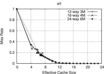
3.4 Profiled cache miss rate corresponding to effective cache size for different cache configurations. . . 31
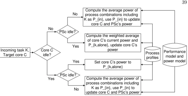
4.1 Algorithm for power estimation for process assignment. . . 39
4.2 Power model validation on 4-core server. . . 42
5.1 System architecture for P-DVFS. . . 61
5.2 Processor frequency as a function of the number of instructions retired for (a) the optimal solution, (b) P-DVFS, and (c) F-DVFS during “mcf” execution with a performance degradation ratio of 20%. . . 64
5.3 Processor frequency as a function of the number of instructions retired for (a) the optimal solution, (b) P-DVFS, and (c) F-DVFS during “art” execution with a performance degradation ratio of 20%. . . 67
6.1 Microarchitecture of a GPU core in Fermi GTX 480. . . 74
6.2 The CPI per warp breakdown for Parboil benchmarks with GTO schedul-ing. . . 78
6.3 This figure shows the relationship between number of warps, CPI, and IPC 80 7.1 The average CPI breakdown of Parboil benchmarks with different schedul-ing policies: 1. GTO; 2. GTO-TAWS; 3. LRR; 4. GTLS; 5. GTLS-TAWS. 86 7.2 The IPC speedup of Parboil benchmarks of different scheduling policies compared with GTO. . . 87
7.4 The instruction issue percentage of LBM according to warp ID . . . 88
7.5 The CPI breakdown of TPA for 24 warps, 8 warps per CTA. . . 89
7.6 The instruction issue percentage of TPA according to warp ID. . . 89
7.7 The CPI breakdown of MRI for 40 warps, 5 warps per CTA. . . 90
7.8 The instruction issue percentage of MRI according to warp ID. . . 90
7.9 The CPI breakdown of SPM for 48 warps, 6 warps per CTA . . . 91
7.10 The instruction issue percentage of SPM according to warp ID. . . 91
8.1 Kernels from different Parboil benchmarks exhibit significantly different utilization of hardware resources and function units on a GPU core, pos-sibly indicating that co-scheduling multiple kernels (with complementary resource utilization) on the same GPU core might improve PLP. Occu. and A.Occu. are short for Occupancy and Achieved Occupancy. . . 94
8.2 Average throughput speedup (G-Mean) and average memory stall rate for existing inter-core and intra-core multitasking. Note MS and NMS are short for MEM-S and Non-MEM-S. . . 97
8.3 High-level view of proposed intra-core multitasking technique. . . 100
8.4 Breakdown of average GPU stall rate for kernels executing on the baseline architecture. TLP stalls occur when no active warp is available. PLP stallsoccur when active warps are available but the scheduler cannot issue an instruction to a particular pipeline due to a structural hazard (e.g., the pipeline is stalled due to excessive unresolved off-chip memory accesses or a full pipeline is still busy executing previously-issued instructions). . 101
8.5 Average utilization of SP, SFU, and MEM in the baseline architecture. . 102
8.6 The tail effect results in reduced achieved occupancy and IPC for single kernel execution and inter-core multitasking. . . 103
8.7 ICMT Architecture with increased frontend bandwidth and PMIQ. . . . 107
8.8 Average throughput speedup (G-Mean) of co-scheduled kernels with dif-ferent scheduling mechanisms. . . 108
8.9 Average issue stall due to memory contention with different scheduling mechanisms. . . 110
nisms. . . 112 8.11 ICMT can mitigate the tail effect, resulting in sustained occupancy and
higher throughput. . . 112 8.12 IPC speedup by increasing front-end throughput with different scheduling
mechanisms. . . 113 8.13 Breakdown of IPC and utilization under intra-core multitasking of<STE,
SPM> with various CTA partitions. “S-” indicates memory stalls and “U-” indicates effective utilization. . . 114 9.1 An example of multitasking within SMs w/ (HIS, BL) pair. (a)SIMT
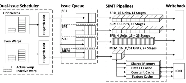
pipeline utilization of two kernels running alone and within SMs multi-tasking w/ 3 different kernel partitions. (b) Avg. pipeline utilization w/ different kernel partitions (c) Occupancy breakdown w/ different kernel partitions (d) Avg. system performance improvement w/ different kernel partitions . . . 119 9.2 (a) Overall System Framework of Fine-grained Kernel Mixing and Grid
Partitioning Technique, (b) Hardware Modification on Dual-Issue Scheduler121 9.3 Detailed Mean Value Based Performance Model . . . 122 9.4 Determining throughput for mixed kernels: (a) Pipeline constrained
sce-nario; (b)Parallelism constrained scenario. . . 123 9.5 Flow of inactive warp through a queuing system . . . 127 9.6 DAG Data Dependency Example: (a) Original DAG Graph; (b) DAG
Graph After Forward Trace; (c) Critical Data Dependency DAG Graph 128 9.7 (a) CD3 histogram of AES; (b)Pinactive data(x) of AES . . . 131
9.8 CalculateingTinactive data . . . 132
9.9 Pinactive data(x) of the Benchmarks . . . 137
9.10 Throughput Improvement of BL Mixing with Other Benchmarks . . . . 139 9.11 Throughput Improvement Different Kernel Partitions in (AES,BL) Pair 140 9.12 Average Throughput Improvement of Benchmarks . . . 140 9.13 Effects of Inter-Warp Scheduling of MUM with Other Benchmarks . . . 141
Chapter 1
Introduction
High-performance computing systems are commonly seen. Typical high performance computing systems include stationary desktop computers, workstations, and servers. Often coupled with multi-core CPUs and GPUs with abundant on-chip and off-chip memory, these modern computing systems have become immensely powerful platform to handle an variety of heterogeneous applications and tasks simultaneously. However, it is no easy task to formalize and solve the problem of optimizing performance and en-ergy consumption for such heterogeneous, potentially data-intensive, workloads running on modern high performance computing systems composed of heterogeneous complex multi-core resources (CPUs and GPUs). To properly tackle this problem, we need a set of optimizing techniques that can address the following challenges:
1. Shared resource allocation, wisely distribute resource shared among different work-loads to avoid significant performance degradation relative to what they could achieve running in a contention-free environment.
2. Workload scheduling, assign workload to different resource sharing clusters to improve shared resource allocation within the resource sharing cluster.
3. Power delivery and voltage control, employ dynamic voltage and frequency scal-ing to match workload behavior to required performance level for best energy efficiency.
The advent of heterogeneous CPUs and GPUs system greatly complicates the three 1
challenges above, and they still remain unsolved despite significant research efforts ded-icated to the problems. Our goal is to consider them together and provide a compre-hensive analysis and technique that allows dynamic performance-aware, energy-efficient management for heterogeneous workloads running in modern high-performance com-puting system.
We take a holistic view of performance, power and resource management in modern computing systems by considering managements at different levels: workload scheduling among resource sharing clusters (Note that we refer to these resource-sharing clusters as memory domains because the shared resources mostly have to do with the memory hierarchy [1]), resource allocation within resource sharing clusters and DVFS-related control within the same voltage/frequency domain.
Existing work in this area addressed the three levels and tried to solve them individ-ually. To simplify the analysis, they usually ignore the impacts between different levels. For instance, pre-core DVFS control without considering the impact of cache contention that caused by the frequency scaling of the processes running concurrently [2] [3], man-age cache partition for throughput optimization without considering local frequency/ voltage scaling [4] To the best of our knowledge, there is very no previous work handles three levels together and very limited work considers the interdependency among each other [1][5].
We believe the following technical contributions are necessary to accomplish the goal of near optimal management of heterogeneous workloads (1) accurate modeling to illustrate the impact of resource contention and indicate the cost of local control policy; (2) efficient local control management and shared resource allocation for opti-mization in energy consumption and performance; (3) performance- and power-aware workload scheduling, jointly considering multiple metrics such as performance, energy consumption, and fairness etc..
1.1
Modeling High-Performance Computing Systems
Modeling high-performance computer systems is a difficult task. Typically, there are four major challenges when designing such models: (1) models need to be accurate. Although model estimation errors are tolerable or addressable through proper guard
banding in many applications, inaccurate estimation results will reduce the usability of such models. (2) Models need to be fast. Significant performance overhead prevents them from being used during runtime, making them inapplicable to many scenarios. In addition, when integrated with optimization techniques, slow models can lead to diminishing returns, or in extreme cases, render the entire optimization technique unus-able. (3) The model construction process should be easy and automatic. Ideally, such modeling techniques should require no changes to the underlying hardware or operating system (OS) so that they can be applied to a variety of systems with different architec-tures. (4) The models should be scalable. The first requirement implies that the model designers must carefully test the models to ensure that the model estimation errors are small in all cases. A designer can improve model accuracy by incorporating more details into the model and simulating the interactions among different model compo-nents. However, this leads to higher computational complexity and therefore conflicts with the second requirement. In addition, the amount of inter-component interactions grows exponentially as more and more cores are integrated into the system. Hence, this approach cannot scale and thus conflicts with the last requirement. Similarly, the model performance can be improved by implementing it on hardware. However, this conflicts with the third requirement. Therefore, designers need to think carefully about the tradeoffs among the aforementioned attributes of the models to develop one that satisfies all the requirements.
Although there are many challenges when designing the models, it is usually worth the effort. Roughly speaking, models can be categorized into design-time models, assign-time models, and run-assign-time models. Design-assign-time models such as power grid models and IC thermal models can help designers to validate the correctness of their decisions during chip design. For example, understanding the thermal implications is essential because early-stage architectural decisions can significantly affect the design of cooling solutions. Assign-time models can predict the impact of process assignment on system metrics such as performance and power, helpful for designing intelligent assignment algorithms. Run-time models such as performance and power models enable system administrators and optimizers to dynamically monitor and predict changes in these runtime parameters, usually with little or no changes to the underlying hardware or applications. Furthermore, all these models have the potential to reveal the bottlenecks
in the system, thus motivating new software and hardware optimization techniques. Finally, modeling techniques is usually the first step toward optimization. In fact, all the optimization techniques proposed in this dissertation are motivated by the modeling techniques, most of which also heavily rely on these models. The ongoing move from single-core to heterogeneous architecture with CMPs and GPUs leads to more complex system architecture and applications, further emphasizing the need for fast and accurate models. In the future, processors are likely to integrate several tens or hundreds of cores on a single chip and probably requires a network on chip. Intel’s recently unveiled 48-core chip is one such example. Without modeling and techniques similar to those described in this dissertation, it is very difficult, if possible at all, to develop optimization algorithms for such systems.
1.2
Optimizing High-Performance Computing Systems
Optimization techniques for high-performance computers are equally, if not more, im-portant than modeling techniques. There are numerous attributes in high-performance computers designers attempt to optimize, e.g., performance, power consumption, tem-perature, and energy. Therefore, optimization techniques have a direct impact on user experience or system monetary cost by optimizing these attributes. It is usually possible to optimize one metric at the cost of another. However, this requires that the designers understand the trade-offs among various system metrics when developing such opti-mization techniques. There has been extensive studies on system-level optiopti-mization techniques for high-performance computing systems (see Chapter 5, Chapter 7, and Chapter 8). However, a large number of existing techniques only optimizes one metric and completely ignores other system metrics. Few algorithms that attempt to opti-mize a metric while constraining others either make unsubstantiated claims without resorting to accurate models, or rely on over-simplified models that produce inaccurate predictions and degrade the quality of optimization results. In our research, we care-fully evaluate the trade-offs among various system metrics and design the optimization techniques based on accurate models when applicable.
1.3
Scheduling High-Performance Computing Systems
The emerging trend of multi-core CPUs and GPU systems allow more tasks running simultaneously, it’s also getting more important to have some performance- and power-aware workload scheduling techniques, jointly considering multiple metrics such as per-formance, energy consumption, and fairness etc.. Such workload scheduling techniques need an accurate performance model to effectively predict the congestion suffered by running multiple tasks concurrently, and performance degradation from each individual tasks. Moreover, moving to the GPU side, workload scheduling technique not only need to determine which workload to scheduling together, but also need to figure out how much resource to be allocated on each workload. Overall, combining a high level work-load scheduling algorithm with a set of local optimization techniques, is the ultimate solution to achieve a near optimal result given metrics such as throughput, energy etc..
1.4
Dissertation Overview
The rest of the dissertation is organized as follows.
Chapter 2–Chapter 5 focus on performance, power modeling and optimization tech-niques for CMPs. Chapter 2 gives an overview of the parameters that influence per-formance and power. We then describe the perper-formance and power implications in modern CMP system. Chapter 3 describes a shared cache aware performance model for CMPs. We also provide an automated technique to collect process-dependent in-formation needed by CAMP without resorting to simulation. Chapter 4 describes a system-level shared cache aware power model and an integrated model for fast and ac-curate power estimations during assignment in a multi-programmed CMP environment. Chapter 5 describes a predictive on-line dynamic voltage and frequency control (DVFS) algorithm that achieves close-to-optimal energy savings with a bounded performance degradation ratio.
Chapter 6–Chapter 9 focus on performance modeling and optimization and schedul-ing techniques for GPUs. Chapter 6 provides a thorough analysis on per-warp CPI breakdown, and identifies out all the key factors that govern GPU throughput from a single warp perspective. Chapter 7 proposes a new two-level priority scheduling policy
to improve performance in single kernel scenario. Chapter 8 proposes ICMT, a full, de-tailed solution for intra-core multitasking for GPGPUs, including architectural support and a contention-aware workload scheduling algorithm that improves TLP and PLP in a balanced fashion. Chapter 9 proposes a new contention-aware analytical perfor-mance model that can provides a fine-grain workload scheduling decision for intra-core multitasking, including detailed resource allocation from co-scheduled workloads.
In the end, we summarize the contributions of the work presented in this dissertation in Chapter 10.
Chapter 2
Multi-core CPU Overview
Performance and power issues are important challenges for the development of high-performance processors. As the industry has shifted their focus from single-core proces-sors to CMPs, new performance and power model are desired. This chapter examines the impact of the current architecture paradigm shift on various modeling techniques and provides insights and motivations for the techniques proposed in Chapter 3–5.
The rest of this chapter is organized as follows. Section 2.1 gives an overview of the fundamental parameters that influences performance and power, many of which must be accounted for in the models to generate accurate estimations. Section 2.2 briefly summarizes CMP architecture background. Section 2.3 provides a motivation example.
2.1
Introduction
The performance of a computer can be defined as the amount of time required to accom-plish one unit of work with one unit of resource. Not surprisingly, the performance of a chip is closely related to its clock frequency, which largely depends on the propagation delay of the transistors on the critical path, affected by supply voltage, temperature, and technology [6]. However a computer’s performance cannot be solely determined by its chip’s clock frequency; other factors such as instruction-level parallelism, thread-level parallelism, off-chip memory access latency, resource contention all contribute to the system performance.
The power consumption can be decomposed into dynamic power and static power.
Dynamic power consumption is caused by the charging and discharging events during voltage transitions in transistors. It scales quadratically with the supply voltage and linearly with the frequency of energy-consuming transitions. Static power, on the other hand, is independent of the frequency of such transitions. However, it has an expo-nential dependence on the supply voltage and temperature. Researchers have proposed numerous techniques to reduce the soaring power of computer systems, among which are dynamic voltage and frequency scaling and clock modulation [7, 8].
2.2
Background
CMP processor is composed of two or more independent CPU cores, thereby allowing more parallelism than single-core architecture. Each CPU core has its own private L1 caches, with the last-level cache being shared among all the cores to improve perfor-mance by supporting on-chip inter-process communication and allowing heterogeneous allocation of cache to processes running on different cores. However, a process may evict the data belonging to other processes with which it shares cache space, known as the cache contention problem. Intuitively, simultaneously running processes may influence each other’s performance through sharing the cache. Furthermore, the performance (and indirectly power) impact is non-uniform, as the cache-sharing processes may have distinct memory access patterns. This requires that the performance model and power model for CMP systems explicitly account for the cache contention problem in addition to the time sharing problem in single-core systems.
2.3
Motivation
Cache sharing among processes running on different cores of a CMP can hide inter-process communication latency and improve cache utilization. This improvement is un-dermined by cache contention among concurrently running processes. To illustrate this effect, we wrote a syntheticstressmark that accesses the last-level cache very frequently. The stressmark is intentionally designed to exhibit extreme memory access behavior, for use in characterization. The stressmark is run concurrently with the process under
0.8 1 1.2 1.4 1.6 1.8 2 2.2 2.4 0 0.1 0.2 0.3 0.4 0.5 0.6 0.7 0.8 0.9 1
Normalized Execution Time
Cache Misses per L2 Access art mcf bzip2 swim equake mesa vpr ammp mgrid applu
Figure 2.1: Impact of stressmark on performance of processes sharing case with it.
evaluation, on another core sharing the same cache. By varying the memory access be-havior of the stressmark, we can change the number of last-level cache misses per cache access (MPA) for the stressmark, thereby controlling and measuring the performance impact on the other concurrently running process.
Figure 2.1 illustrates the relationship between the execution time, normalized to that when running the process alone, and MPA of the stressmark when it is run con-currently with each of 10 SPEC CPU2000 benchmarks. The relationship between MPA and execution time depends on the application. For example, with an MPA value of 0.35, the normalized execution time of art increased by 120% while that of mesa only increased by 1.5%. This demonstrates that the impact of cache contention on per-formance is application-dependent. Accurately predicting the perper-formance and power consumption implications of assigning a particular set of processes to a CMP therefore requires a model that captures the variation in cache access and contention behavior among processes.
Chapter 3
Performance modeling on CMPs
The ongoing move to chip multiprocessors (CMPs) permits greater sharing of last-level cache by processor cores, but this sharing aggravates the cache contention problem, potentially undermining performance improvements. Accurately modeling the impact of inter-process cache contention on performance and power consumption is required for optimized process assignment. However, techniques based on exhaustive consider-ation of process-to-processor mappings and cycle-accurate simulconsider-ation are inefficient or intractable for CMPs, which often permit a large number of potential assignments.
In this chapter, we propose CAMP, a fast and accurate shared cache-aware perfor-mance model for multi-core processors. CAMP estimates the perforperfor-mance degradation due to cache contention of processes running on CMPs. It uses reuse distance his-tograms, cache access frequencies, and the relationship between the throughput and cache miss rate of each process to predict its effective cache size when running concur-rently and sharing cache with other processes, allowing instruction throughput estima-tion. We also provide an automated way to obtain process-dependent characteristics, such as reuse distance histograms, without offline simulation, operating system (OS) modification, or additional hardware. We tested the accuracy of CAMP using 55 dif-ferent combinations of 10 SPEC CPU2000 benchmarks on a dual-core CMP machine. The average throughput prediction error was 1.57%.
The rest of this chapter is organized as follows. Sections 3.1 and 3.2 motivate the problem, summarize our contributions and present related work. section 2.3 describes
CAMP. section 3.4 introduces an automated way to characterize process memory ac-cess behavior to permit later prediction of cache contention. section 3.5 presents and discusses the experimental validation process and results. Finally, section 3.6 concludes this chapter.
3.1
Introduction
In recent chip multiprocessor (CMP) architectures, last-level caches are often shared among cores. This can improve performance by supporting on-chip inter-process com-munication and allowing heterogeneous allocation of cache to processes running on dif-ferent cores. However, a process may cause the eviction of data belonging to other pro-cesses with which it shares cache space. This contention for shared cache space can cause simultaneously running processes to influence each other’s performance. Moreover, the performance impact is non-uniform: it depends on the memory access behaviors of all processes with which it shares cache space.
The importance of inter-process cache contention for CMPs has been recognized in prior work [9, 10, 11]. However, the problem of predicting the impact of cache sharing on application performance during process assignment has been considered by only a few researchers [12, 13]. Knowing the performance implications of alternative assignment decisions can improve their quality. We therefore seek to build a cache contention model that permits fast and accurate performance prediction of processes on CMPs.
The construction of such a model should be easy and automatic; it should not require modifications to existing operating systems (OS) or hardware. Exhaustive offline simulation of process combinations is computationally intractable and should therefore be avoided. Moreover, prior work does not permit accurate prediction of the steady-state cache partition among arbitrary combinations of processes, which is a prerequisite for accurate performance prediction during assignment.
The chapter describes a fast and accurate shared cache aware performance model for multi-core processors (called CAMP). This model uses non-linear equilibrium equa-tions in a least-recently-used (LRU) or pseudo-LRU last-level cache, taking into account process reuse distance histograms, cache access frequencies, and miss rate-aware perfor-mance degradation. CAMP models both cache miss rate and perforperfor-mance degradation
as functions of process effective cache size, which in turn is a function of the memory access behavior of other processes sharing the cache. CAMP can be used to accurately predict the effective cache sizes of processes running simultaneously on CMPs, allow-ing performance prediction with an average error of only 1.57%. We also propose an easy-to-implement method of obtaining the reuse distance histogram of a process with-out offline simulation or modification to commodity hardware or OS. In contrast with existing techniques, the proposed technique uses only commonly available hardware per-formance counters. Finally, we evaluate the generality of CAMP by profiling processes on one CMP and using the resulting models to accurately predict process performance when run on two other CMPs having different cache sizes. All the measurements are performed on real processors.
3.2
Related Work
Past work [14, 15, 16, 17] has considered the problem of adjusting cache partitioning during runtime after process assignment decisions have already been made. In contrast, the goal of our work is to predict the performance implications of process assignment decisions before execution. Other researchers have developed performance prediction models to guide process assignment. However, most [18, 19] addressed cache contention only for uniprocessors on which only a single process may run at a time. The move to CMPs will aggravate the cache contention problem since multiple processes can run on different cores simultaneously.
Resource contention models for simultaneous multithreading (SMT) uniprocessors should be applicable to CMP systems due to the similarity in inter-process resource con-tention. However, existing work on resource contention modeling for SMT processors either suffers from large performance prediction error (20% of instruction throughput predictions deviate by more than 20% from the actual instruction throughput) [20] or requires modifications to the underlying hardware [21]. To the best of our knowl-edge, existing performance models for SMT processors do not support accurate runtime performance prediction. Although the similarity of cache effects for CMPs and SMT processors suggests that the modeling technique described in this chapter might also be accurate for SMT processors, we have not yet experimentally tested this hypothesis.
Researchers have also considered addressing the performance prediction problem using offline simulation [22] or modifications to the existing hardware or operating sys-tem [23]. For example, Suhet al.[16] proposed to add a hardware counter to each cache way and use them to determine the reuse distance histogram. Our goal is runtime pre-diction of the performance of a process concurrently running on a shared-cache CMP, without requiring prior characterization.
Tam et al. [24] previously developed a technique to predict miss rate as a function of cache size by using built-in hardware performance counters, with a primary goal of supporting on-line optimization of cache partitioning among processes. They do not explain how to use miss rate curves to predict instruction throughputs for processes sharing cache space. Also, their approach relies on performance counters peculiar to the POWER5 architecture.
Chandra et al. [13] proposed three analytical models to predict miss rates for pro-cesses sharing the same cache. Their models use the reuse distances and/or circular sequence profiles for each thread to predict inter-thread cache contention. These mod-els require knowledge of the steady-state L2 cache access frequency of a process when concurrently running with other processes. In reality, obtaining this information without running or simulating all potential combinations of concurrent cache-sharing processes is impractical.
Chen et al. [12] proposed a two-phase approach for performance prediction. In the first phase, the access frequency of a process running alone is used to estimate performance. In the second phase, the performance estimates from the first phase are refined to consider the implications of cache contention. The models proposed in each paper require processing circular memory access sequences, which must be obtained by tracing execution with an instruction-set simulator or non-standard detailed access tracing hardware.
3.3
Analytical Model
This section describes the main components in CAMP, namely its performance model, effective cache size estimation technique, and steady-state condition estimator.
3.3.1 Background
In this section, we define some basic terms that will be used throughout this chapter. Our study will consider an N-core processor with an L2 last-level on-chip cache. In the rest of the chapter, we refer to “L2 cache” as “cache”. A set-associate cache is broken intosets, each of which has space for multiplelines, i.e., the minimal unit of data fetched by or evicted from a cache. The number of lines per set is the cache’s associativity, i.e., its number of ways. A line at a particular location in memory is associated with a set and may be fetched into any line in the set.
Effective Cache Size
When multiple processes share a cache, they compete for limited space. The division of cache space among processes is influenced by characteristics of the concurrently running processes, such as cache access frequency and sequential data access patterns. We define effective cache sizeof processito be the average number of ways occupied by the process in a set, denoted as Si. Therefore,
N
X
i=1
Si =A, (3.1)
where N is the total number of processes sharing the cache and A is the number of ways in the cache. Note that Si is a real value in our model because it represents the
average number of ways process i occupies in a set during prolonged execution. If the cache access behavior of all processes is static, then Si will be stable. We define this as
the steady-state condition.
Reuse Distance
We define the reuse distance, Rj, of cache line j to be the number of distinct cache
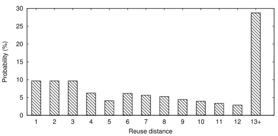
lines within the same set accessed between two consecutive accesses to line j. A reuse distance histogram represents the distribution of cache line reuse distances for an entire shared cache. Given an A-way set-associative cache, Figure 9.7 shows a reuse distance histogram for themcf application (see section 3.5). Thex-axis shows the reuse distance and they-axis shows the normalized frequencies of the associated reuse distances. The first bar in the histogram, i.e., hist1, gives the probability that a most-recently-used
0 5 10 15 20 25 30 1 2 3 4 5 6 7 8 9 10 11 12 13+ Probability (%) Reuse distance
Figure 3.1: Cache line reuse distance histogram for mcf application.
line will be accessed again, while the last bar, i.e., hist13+, gives the probability that
the data for the next cache access does not exist in the most-recently-used 12 lines, which can be denoted as P∞
k=13histk. Hist∞ is the probability that the data in the
line is never accessed again. Note that hist∞ can be very large for some streaming
applications. For process iwith an effective cache size ofSi, all accesses to the cache
lines with a reuse distance larger thanSi result in cache misses. Hence, the probability
of a cache access resulting in a miss for process i with an effective cache size ofSi can
be expressed as follows.
MPAi(Si) =
Z ∞
Si
histi(x)dx. (3.2)
Note that histi(x) is a continuous function derived using linear interpolation of the
discrete histogram to support estimation for non-integer average reuse distances.
3.3.2 Problem Formulation and Assumptions
The cache contention prediction problem can be formulated as follows: given N pro-cesses assigned to cores sharing the sameA-way set-associative last-level cache, predict the steady-state cache size occupied by each process during concurrent execution. Note that the steady-state cache size can be directly translated to performance, as illustrated by Equation 3.2. Solving this problem is helpful for process assignment and migration in a CMP environment because it allows one to predict the consequences of tentative process assignment and migration decisions. However, accurate prediction of process
performance is challenging because there are many combinations of processes that may share the same cache.
We make the following assumptions.
1. For each process, we assume that data accesses are uniformly distributed across all cache sets. The temporal cache access behaviors such as number of cache accesses per second (APS) and the reuse distance histogram (see section 6.2) are assumed to be stationary. In the case of multiple non-repeating phases with distinct memory access patterns [25], non-repeating phases should be modeled separately.
2. We assume no hardware prefetching. Hardware prefetching predictively fetches cache lines based on access patterns, potentially complicating the model. As such, the model might be inaccurate for systems using prefetching. However, we argue that prefetching is of limited value on CMPs with constrained processor-memory bandwidth. For the 10 benchmarks used in this work, the average improvement was 3.25%, and only equake benefitted significantly.
3. We do not explicitly model the effect of kernel thread and instruction accesses on cache contention but note that the resulting technique remains accurate in the presence of these accesses.
4. The cache uses an LRU replacement policy. Although most modern caches use pseudo-LRU policies, assuming LRU still permits high prediction accuracy. Although these assumptions simplify the explanation of our analysis, we do not rely on them but instead “close the loop” by evaluating the resulting prediction technique on real systems for which the assumptions may not hold. Finally, we consider a multi-programmed environment and therefore neglect communication among processes. Our analysis will hold for applications in which there is little communication among processes assigned to separate cores.
3.3.3 Performance Model
The average number of cache accesses per second (APS) reflects how aggressively a process competes for cache space. All other things being equal, a process with high
APS will generally take up more space in a shared cache than a process with low APS.
APS = API
SPI, (3.3)
where API is the number of cache accesses per instruction and SPI is the number of seconds per instruction. API is a process property: given the same input data, the API of a process is fixed. On the other hand, SPI is largely affected by the number of cache misses per second (MPS). The latency per instruction, i.e., seconds per instruction, can be decomposed into two parts: on-chip latency due to computation and off-chip latency caused by main memory and disk accesses. When the CPU frequency remains constant, the on-chip latencies per instruction are approximately constant for a process. As shown in Figure 2.1 we experimentally determined that SPI can be expressed as a linear function of MPA.
SPI =α·MPA +β, (3.4)
where α and β are parameters that can be obtained during offline characterization.
3.3.4 Estimating Effective Cache Size After n Accesses
In this section, we use the reuse distance histogram of a process to derive its effective cache size. Consider the number of distinct cache lines, s, (i.e., the effective cache size of the process) aftern accesses in one set. Note thatsis essentially the effective cache size,Si, as defined in section 3.3.1. Given thatPs,nis the probability of havingsdistinct
cache lines afternconsecutive cache accesses,Phit,sis the probability that a cache access
will result in a cache hit when the process already has s cache lines, and Pmiss,s is the
probability that a cache access will result in a miss when the process has scache lines, noting scan never be greater than n, the following recursive equation can be derived:
Ps,n=Ps,n−1·Phit,s+Ps−1,n−1·Pmiss,s−1,1< s≤n. (3.5)
This can be explained as follows. The fact that n cache accesses result in an effective cache size of scan only be the result of one of the following scenarios.
1. In scenario A, the first n−1 cache accesses led to an effective cache size ofsand the nth access resulted in a cache hit. Since the nth access did not lead to an
increase in the effective cache size, it remainss. The probability of this scenario,
P(A), is Ps,n−1·Phit,s.
2. In scenario B, the first n−1 cache accesses lead to an effective cache size of s−1 and the nth access causes a cache miss. In this case, the effective cache size is increased by one, relative to thes−1 lines resulting from the firstn−1 accesses. Thus, the effective cache size will be safter n cache accesses. The probability of this scenario, P(B), is Ps−1,n−1·Pmiss,s−1.
Noting that Ps,n =P(A) +P(B), we can derive Equation 3.5.
Given that MPA(s) is the probability of a cache access missing, given an effective cache size of s, Equation 3.5 can be written as
Ps,n=Ps,n−1·(1−MPA(s)) +Ps−1,n−1·MPA(s−1). (3.6)
Note that P1,1 = 1 because the first cache access always causes a cache miss and
re-placement and 1 < s≤n. Assuming the process reaches steady state after naccesses, and given that Gi(n) is the effective cache size for process iafter naccesses, we have
Gi(n) = n
X
s=1
(Ps,n·s). (3.7)
Note that Gi(n) is a monotonically increasing function ofn. Therefore, given the
effec-tive cache size of processi,Si, we can deduce the number of cache accessesnneeded for
the process to reach steady state using the inverse function of Gi(n), i.e.,n= G−i 1(Si).
3.3.5 Steady-State Conditions
Given a cache with an LRU-like replacement policy, it is reasonable to assume that at timet, we can always find a duration T such that data accessed before timet−T have been evicted and data accessed during [t−T,t] are presently in the cache. To determine the effective cache size, we are only interested in data accessed during [t−T,t]. Since none of these accesses will evict any data lines accessed during [t−T,t], it is as if the data were written to an empty cache with no cache misses during [t−T, t]. Thus, Equations 3.6 and 3.7 hold. Note that these accesses may still evict cache lines accessed before t−T. We assume the partition among processes resulting from data accesses
from all co-running processes within [t−T,t] is the same as that when all the processes reach steady state. By computing the cache size of each process resulting from data accesses within [t−T, t], we can determine process effective cache sizes. Hence, the effective cache size of process i, denoted as Si, corresponds to the expected cache size
determined by the most recent APS·T cache accesses for processi. Thus, the effective cache Si is written as Gi(APSi·T). Conversely, APSi can be expressed as G−i 1(Si)/T.
From Equation 3.3 and 3.4, we can derive the following equation: APSi = G−i 1(Si) T = APIi αi·MPAi(Si) +βi . (3.8) Therefore, T = G −1 i (Si)·(αi·MPAi(Si) +βi) APIi . (3.9)
Note that Equation 3.9 holds for any process i, wherei∈ {1,2,· · · , N}, given that
N is the total number of processes. Combined with Equation 3.1, we have G−11(S1) G−j1(Sj) − API1·(αjMPAj(Sj) +βj) APIj·(α1MPA1(S1) +β1) = 0,∀Nj=1, (3.10) and N X i=1 Si−A= 0, (3.11)
where G−i 1(Si) and MPAi(Si) are application-dependent non-linear functions ofSi. We
solve Equation 3.10 using Newton–Raphson iteration, a standard numerical method for finding the roots of non-linear equations. Note that the number of ways in a cache (A) and number of cores (N) are each fewer than 10. G−i 1(Si) and MPAi(Si) are monotonic
functions of Si, so we can solve Si for process i accurately within several iterations,
where i ranges from 1 to N. The initial guess also affects the computational cost. In our experiments, we find that initially guessing that the effective cache size of a process
iis proportional to its APS allows quick convergence to an accurate solution.
3.4
Automated Profiling
In this section, we first explain how to obtain the reuse distance histogram of a process. We then describe how to derive other parameters such as API and MPA. After that, we
give details about the automated profiling process. Finally, we indicate possible sources of prediction error.
3.4.1 Reuse Distance Profiling
Process reuse distance histograms play a central role in the proposed performance mod-eling technique. It would be possible to extract the reuse distance histograms of pro-cesses via simulation, and CAMP would dramatically improve estimation speed even if simulation were used for initial characterization; however, there is a faster alternative.
Most modern processors have built-in hardware performance counters (HPCs) that record information about architectural events such as the number of instructions retired, number of last-level cache accesses, and number of last-level cache misses [26]. Therefore, we can gather information about parameters such as SPI and MPA accurately. However, existing hardware or software resources do not directly provide reuse histogram data. We now explain the process of deriving reuse histogram data from directly monitored parameters.
Consider two processes running on separate cores sharing anA-way last-level cache. We assume if one process occupies l ways in a cache set, the concurrently running process will occupy A−l ways. Based on Equation 3.2, we can compute the effective cache size of astressmark with a controlled MPA and a known reuse distance histogram. We obtain the reuse distance histogram of a process (denoted as B) as follows. Run the stressmark along with B multiple times. In the lth run, we tune the parameters in the stressmark to change the effective cache size, denoted as Sstress,l. Record B’s MPA in
each run, denoted as M P AB,l, where l ∈ {1,2,· · ·, A}. Given that SB,l is process B’s
effective cache size in thelth run, and considering thelth and thel+ 1st runs, we have
M P AB,l+1 = Z ∞ SB,l+1 histB(x)dxand M P AB,l = Z ∞ SB,l histB(x)dx. (3.12)
See the discussion after Equation 3.2 for the definition of hist(x). Hence, we can estimate the probability of process B having an effective cache size ofSB,l as
Algorithm 1 Stressmark with k-Way Occupation
1: Set is the number of cache sets.
2: Step is the number of integers per cache line.
3: S[Set·Step·k] is an array of integers.
4: Index ← {s1, s2,· · ·, sn}
5: The following loop loads a predefined random sequence into Index.
6: for j= 0 : n−1 do
7: flag←Index[j]
8: T ←&S[flag·Set·Step]
9: fori= 0 : Set−1do
10: readT[i·Step]
11: end for
12: end for
By varyingSB,l from 1 toA, we can estimate the probability at each effective cache size,
thus allowing us to construct the reuse distance histogram. Since we can not control
SB,l directly, in practice we adaptively tune the effective cache size of the stressmark
from run to run. SB,l+Sstress,l=A. Therefore, varying Sstress,l changes SB,l.
As indicated above, the stressmark should have the following properties.
1. High cache access frequency, i.e., high API. API is related to the degree to which a process competes for cache space. In order to estimate the probability of a process having a small effective cache size, the concurrently running stressmark should occupy a large portion of the cache with few cache misses.
2. A uniform reuse distance histogram, i.e., the probability is the same across all possible reuse distances. This makes it easy to compute the effective cache size given an MPA value. In addition, given a pseudo-LRU cache replacement policy, cache lines other than the least recently used will sometimes be evicted. Having a uniform reuse distance histogram minimizes the impact of this potential prob-lem because the replacement noise will affect cache lines with all reuse distances equally.
The pseudo-code of the stressmark is shown in 1, where Set is the number of sets in the cache, Step is the number of integers per cache line. Index[n] is an integer array whose elements are uniformly distributed from [1, k], which contains a random access location sequence. In order to maintain high cache access frequency for the stressmark,
we pre-generate these arrays. Note that in Line 10 in 1, two consecutive reads are Step elements apart to ensure a 100% L1 cache miss rate. Since the stressmark randomly accesseskcache lines within a cache set, the effective cache size of the stressmark is ex-pected to be k. However, this may not be very accurate due to conflict misses between the stressmark and the process of interest. In reality, we use Equation 3.2 to esti-mate the effective cache size of the stressmark, i.e.,Sstress = MPA−1(MPAstress), where MPAstress is the MPA of the stressmark and MPA−1() is the inverse function for MPA in Equation 3.2 that converts MPA to an effective cache size, i.e., MPA−1(MPA(x)) =x.
3.4.2 Automated Parameter Estimation
In this section, we describe how we calculate parameters such as API and SPI for a process. Given anA-way associative cache, in order to get the reuse distance histogram for a process, we run the stressmark concurrently with the process A times. In the lth run, we setktolfor the stressmark in 1. Since API is fixed for a process with the same input data, given thatAPIl is the process’s API in the lth run, the average API of the
process can be estimated as
API = PA
l=1APIl
A . (3.14)
Similarly, we can getA pairs of a process’ MPA and SPI values from theAruns. Given that M P Al and SP Il are the average MPA and SPI of the process in thelth run, the
α and β in Equation 3.4 can be determined using linear regression, i.e.,
α= A·( PA l=1MPAl·SPIl)−( PA l=1MPAl)( PA l=1SPIl) A·(PA l=1MPAl2)−( PA l=1MPAl)2 (3.15) andβ = ( PA l=1SPIl)−α·( PA l=1MPAl) A . (3.16)
Note that most programs have repeating phases with periods ranging from 200 ms to 2,000 ms [25]. Numerous works exist on phase detection, i.e., finding the time at which the process switches from one phase to another. Since the process behavior is by defi-nition similar within a phase, one set of parameters per phase is sufficient. In the rest of the chapter, we will treat processes as having a single phase each to simplify expla-nation. Note that the proposed technique is also suitable for multi-phase processes, for which each phase may have a different set of extracted parameters.
Process characterization can be automated as follows. First, run the stressmark along with the process A times, varying the effective cache size. AfterA runs, API,α,
β, and the reuse distance histogram can be estimated using Equations 3.13–3.16. These four parameters form the feature vector of a process. Given the feature vectors of two processes, we can predict their effective cache sizes when sharing a cache, which in turn can be translated to SPI values using Equations 3.2 and 3.4. Note that the SPIs for the two processes are predicted without actually running them concurrently. Hence, given N processes for assignment toN cores, onlyN feature vectors are needed (O(N) complexity). These vectors can be used to predict the performance of any subset of the
N processes during assignment (2N −1 combinations). Thus, the proposed technique is dramatically more efficient than one requiring simulation or execution of 2N −1 combinations of processes.
3.4.3 Potential Sources of Error
There are two primary sources of error in the proposed technique: error in histogram estimation and error in linear regression analysis. We will explain these error sources now, but note that even with these error sources, the proposed technique is highly accurate (see section 3.5).
When estimating the reuse distance histogram for a process, it is very difficult to capture the probability corresponding to a reuse distance close to 0 because the con-currently running stressmark cannot consume all of the cache space. Similarly, the estimation for a reuse distance close to A may also have some error. In practice, we assume a uniform distribution for reuse distances close to 0 or A. Linear interpolation, given an assumed miss rate of 1 at an effective cache size of zero, is used for very small effective cache sizes. In addition, the probability of reuse distances larger than A can-not be captured by our technique. Hence, we extrapolate this probability based on the derivative of the probability density function at a sample point close to A.
Error may also be introduced due to noise in sample parameters. When the<MPA, SPI>pairs gathered during profiling are clustered within a small region, linear regres-sion may lead to inaccurate estimation of coefficients due to noise. We addressed this problem by bounding the step size during Newton–Raphson iteration when solving for the effective cache size (see Equation 3.10), permitting convergence.
Table 3.1: Intel P8600 Specification
Item Specification Number of chips 1
Number of cores per chip 2 Frequency 2.40 GHz
L1 ICache (Private) 32 KB, 64 B line, 8-way associative L1 DCache (Private) 32 KB, 64 B line, 8-way associative L2 Cache (Shared) 3 MB, 64 B line, 12-way associative
3.5
Evaluation Methodology and Results
In this section, we first describe our experimental setup. We then present the exper-imental results for model validation. We contrast the proposed technique with other potential methods of predicting CMP cache contention among processes and indicate which features of the proposed approach permit high prediction accuracy.
3.5.1 Experimental Setup
We evaluated our technique on a computer equipped with an Intel Core 2 Duo P8600 processor and the Mac OS X 10.5 operating system. The system parameters are listed in Table 3.1. We used Shark, a built-in profiling tool, to sample performance counters at a period of 2 ms. The samples are used for calculating parameters (e.g., API, MPA, and SPI) on each core. We used the SPEC CPU2000 benchmark suite, which contains 26 benchmarks. Since validating all 351 pairwise combinations would be costly, we instead selected a subset containing five CPU-intensive and five memory-intensive benchmarks, and considered all pairwise combinations of these ten. We recorded the program phase information for each benchmark during pre-characterization. Experimental results in-dicate that all but two benchmarks have only one significant phase, as defined by our parameters of interest. The longest phases in art and mcf were used. We can thus address the prediction problem one phase at a time using phase detection algorithms, as described in subsection 3.4.2.
Table 3.2: API,α, and β for Different Benchmarks
Benchmark art mcf bzip2 swim equake mesa vpr ammp mgrid applu API 0.0225 0.0733 0.0044 0.0116 0.0074 0.0013 0.0102 0.0092 0.0018 0.0018
α(×10−9) 446 134 99.9 -99.6 60.5 30.7 306 243 0.609 3.12
β(×10−7) 1.34 5.86 1.50 1.97 2.28 1.55 1.65 1.83 1.28 1.15
3.5.2 Pre-Characterization
As indicated in subsection 3.4.2, we first run the stressmark concurrently with each benchmark on two different cores 12 times to derive various parameters such as API, MPA, and SPI. Each run lasts 10 s, which has proven sufficient for characterizing these parameters. Note that the working data set size of the stressmark is incremented by 1 way after each run to construct the reuse distance histogram for each benchmark, as described in subsection 3.4.1.
Analyzing API, α, and β
Hardware performance counter readings are analyzed to determine API, α, and β in Equations 3.3 and 3.4. Table 3.2 shows the value for each benchmark. API indicates an application’s capability to compete for cache space. It also indicates whether an application is memory-intensive because higher API is usually associated with more misses per instruction, resulting in more off-chip memory transactions. As indicated in Table 3.2, benchmarks such as art, mcf, vpr, swim, and ammp are memory-intensive. Their APIs are significantly higher than those of the other benchmarks. α indicates sensitivity to cache misses in terms of performance. Equation 3.4 implies that for the same amount of change in MPA, a largerαindicates a larger change in SPI. As shown in Table 3.2, the performance of memory-intensive applications tends to be more sensitive to cache misses than that of CPU-intensive applications, withart being the most cache-miss sensitive benchmark and mgrid being the least cache-miss sensitive benchmark. Note that α is negative forswim. This is because cache contention has little impact on this benchmark’s MPA value, resulting in inaccurate estimation during linear regression when building the SPI model. However, this introduces little error in performance estimation because, as we show later in Figure 3.2, both MPA and SPI are insensitive to effective cache size for this benchmark.
0 0.2 0.4 0.6 0.8 1 0 2 4 6 8 10 12 Miss Rate
Effective Cache Size art 0 0.2 0.4 0.6 0.8 1 0 2 4 6 8 10 12 Miss Rate
Effective Cache Size mcf 0 0.2 0.4 0.6 0.8 1 0 2 4 6 8 10 12 Miss Rate
Effective Cache Size vpr 0 0.2 0.4 0.6 0.8 1 0 2 4 6 8 10 12 Miss Rate
Effective Cache Size mesa 0 0.2 0.4 0.6 0.8 1 0 2 4 6 8 10 12 Miss Rate
Effective Cache Size mgrid 0 0.2 0.4 0.6 0.8 1 0 2 4 6 8 10 12 Miss Rate
Effective Cache Size swim 0 0.2 0.4 0.6 0.8 1 0 2 4 6 8 10 12 Miss Rate
Effective Cache Size ammp 0 0.2 0.4 0.6 0.8 1 0 2 4 6 8 10 12 Miss Rate
Effective Cache Size applu
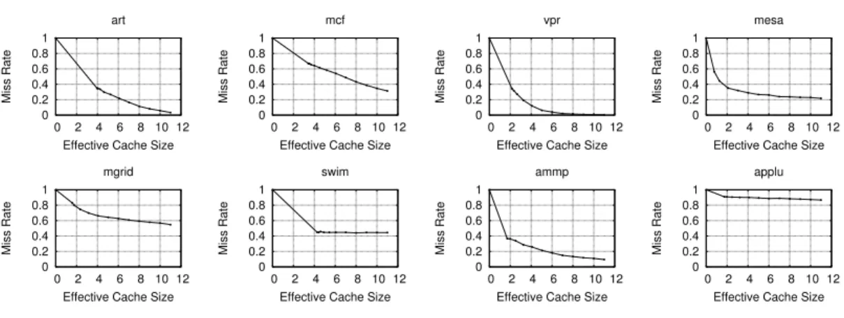
Figure 3.2: Profiled cache miss rate corresponding to effective cache size.
Analyzing Cache Miss Rate
We use the approach explained in subsection 3.4.1 to build the reuse distance histogram for each benchmark, which is then used to predict its cache miss rate as a function of effective cache size. Figure 3.2 illustrates the relationship between cache miss rate and effective cache size for each benchmark. The cache miss rate curves for benchmarks bzip2 andequake are not shown because they are similar to that ofmgrid. The results, from execution on hardware, are consistent with those obtained from simulation [27]. Note that linear approximation is used for leftmost segment of each miss rate curve, for the reasons given in subsection 3.4.3. However, for the benchmarks with high APIs such as swim and applu, the solutions of Equation 3.10 always lie outside this linear region. Therefore, we do not consider this region when analyzing the sensitivities of the cache miss rate curves for any benchmarks. As indicated in Figure 3.2, the cache miss rates of benchmarks such as swim and applu are insensitive to their effective cache sizes in the effective range. Therefore, their performance is only slightly affected when run together with other benchmarks. However, cache miss rates of benchmarks such as art and vpr are very sensitive to their effective cache sizes. Therefore, their performances will be significantly affected by cache contention, although the impact on their performances highly depends on the memory access patterns of the processes running concurrently with them. This indicates the importance of considering application behavior and cache contention during performance prediction on CMPs.
3.5.3 Model Validation
In this section, we validate our technique by using the feature vector, i.e.,<API, α, β>, and reuse distance histogram of a benchmark to predict the performance when run concurrently with another benchmark. Note that feature vectors are determined during pre-characterization. We compare the performances of the two benchmarks during the evaluation period to the predicted performances using the feature vectors of the benchmarks. Note that the approach proposed by Chandra et al. [13] requires the steady-state cache access frequency of a process to be known a priori. We see no practical way to accurately predetermine this value for concurrently running processes. In contrast, our technique determines the steady-state cache access frequency using analysis of performance counter readings, i.e., the proposed technique works correctly using only inputs that are readily available in real systems.
In addition to the proposed technique, we considered and evaluated two alternatives. The first, called Accesses Based (AB), assumes the effective cache size of a process is proportional to APS. Given two processes running on two cores with effective cache sizes ofS1 and S2, the formula to determine effective cache sizes can be written as
APS1 APS2 = S1 S2 = API1·(α2MPA2(S2) +β2) API2·(α1MPA1(S1) +β1) . (3.17)
Note that this model only considers APS. It may be inaccurate if the concurrently running processes have different MPAs or reuse frequencies. The second model, known as Misses Based (MB), assumes thatSiis proportional to MPS. Therefore, the equation
used to determine S1 and S2 is
MPS1
MPS2
= MPA1(S1)·API1·(α2MPA2(S2) +β2) MPA2(S2)·API2·(α1MPA1(S1) +β1)
. (3.18)
The model only considers MPS. Thus it may be also inaccurate if the concurrently running processes have different reuse distance profiles.
Analysis of Results
We examined all 55 possible pairwise combinations of 10 benchmarks: each benchmark is paired with every other benchmark (including another instance of itself) and assigned to the two cache-sharing cores. The measured performance data are then compared to
Table 3.3: Prediction Accuracy for Cache Misses and Performance Degradation
CAMP AB MB
MPA SPI MPA SPI MPA SPI
Benchmark Error >5% Error >5% Error >5% Error >5% Error >5% Error >5% (%) (%) (%) (%) (%) (%) (%) (%) (%) (%) (%) (%) art 1.61 0 3.68 40 4.60 50 10.26 80 5.88 70 18.09 90 vpr 0.88 0 1.48 0 4.70 40 7.67 60 5.89 30 9.24 50 mcf 2.10 10 3.70 20 2.82 10 3.97 40 6.79 40 7.72 70 ammp 2.82 20 3.04 20 4.03 30 4.16 30 5.89 60 6.78 90 bzip2 1.86 10 1.17 0 3.17 20 1.89 0 6.09 60 3.63 30 mesa 4.23 50 0.83 0 4.90 30 0.94 0 7.77 50 1.55 0 swim 0.28 0 0.86 0 0.23 0 0.81 0 0.27 0 0.78 0 equake 0.70 0 0.38 0 0.92 0 0.41 0 1.43 0 0.45 0 applu 1.13 0 0.32 0 0.86 0 0.31 0 1.79 10 0.33 0 mgrid 2.79 10 0.28 0 3.35 20 0.28 0 6.00 40 0.30 0 top 5 average 1.86 8 2.61 16 3.86 30 5.59 42 6.11 52 9.09 66 average 1.86 4 1.57 8 2.94 20 3.07 21 4.78 36 4.89 33
those predicted by AB, MB, and CAMP. AB and MB are not past work. They are in fact alternative prediction models we considered.
Table 3.3 presents the average prediction error in cache miss rate and performance for each benchmark when run simultaneously with each of the 10 benchmarks. The first column lists the benchmarks. Columns 2, 6, and 10 show the average magnitudes of cache miss estimation error for CAMP, AB, and MB. Columns 3, 7, and 11 show the percentage of test cases with a cache miss estimation error larger than 5% among all 10 test cases. Similarly, Columns 4, 8, and 12 indicate the average relative estimation error in performance for the three techniques, while columns 5, 9, and 13 indicate the percentage of test cases with a relative performance estimation error larger than 5% among all 10 test cases for the three techniques. The last two rows correspond to the results for the 5 most memory-intensive benchmarks and all 10 benchmarks, respectively. As indicated in Table 3.3, CAMP has an average of 1.57% performance estimation error over all 10 benchmarks, compared to 3.07% for AB and 4.89% for MB. In addition, only 8% of the cases for CAMP have estimation errors greater than 5%, compared to 21% for AB and 33% for MB. Note that all three models have average performance estimation errors below 5%. This is mainly because all the three models are based on predicting the effective cache size of each benchmark when subject to cache sharing. If one of the two co-running benchmarks are CPU-intensive, e.g., mesa,applu, ormgrid, at least one