Research on Image Generation and Style Transfer Algorithm Based on Deep Learning

ISSN Online: 2165-3925 ISSN Print: 2165-3917

DOI: 10.4236/ojapps.2019.98053 Aug. 28, 2019 661 Open Journal of Applied Sciences

Research on Image Generation and Style

Transfer Algorithm Based on Deep Learning

Ruikun Wang

School of Computer Science and Technology, Tianjin Polytechnic University, Tianjin, China

Abstract

Aiming at the current process of artistic creation and animation creation, there are a lot of repeated manual operations in the process of conversion from sketch to the stylized image. This paper presented a solution based on a deep learning framework to realize image generation and style transfer. The method first used the conditional generation to resist the network, optimizes the loss function of the training mapping relationship, and generated the ac-tual image from the input sketch. Then, by defining and optimizing the per-ceptual loss function of the style transfer model, the style features are ex-tracted from the image, thereby forming the actual The conversion between images and stylized art images. Experiments show that this method can greatly reduce the work of coloring and converting with different artistic ef-fects, and achieve the purpose of transforming simple stick figures into actual object images.

Keywords

Deep Learning, Image Generation, Style Transfer

1. Introduction

At present, the art creation and animation creation process mainly uses sketch-ing first, and then through a series of processes such as colorsketch-ing to form an ac-tual picture. When the style needs to be converted, most of them need to be re-colored, which leads to a large number of repeated manual operations in the process. This paper uses the advantages of deep neural networks, combined with conditional confrontation networks and convolutional neural networks, to au-tomatically implement the process of sketching to physical and style conversion. CNNs are the main methods to solve various image recognition and detection. CNNs minimize the loss function by learning features [1]. Although the feature

How to cite this paper: Wang, R.K. (2019) Research on Image Generation and Style Transfer Algorithm Based on Deep Learn-ing. Open Journal of Applied Sciences, 9, 661-672.

https://doi.org/10.4236/ojapps.2019.98053

Received: July 30, 2019 Accepted: August 25, 2019 Published: August 28, 2019

Copyright © 2019 by author(s) and Scientific Research Publishing Inc. This work is licensed under the Creative Commons Attribution International License (CC BY 4.0).

DOI: 10.4236/ojapps.2019.98053 662 Open Journal of Applied Sciences learning process is automated, it still requires a lot of manpower to design its tags. In contrast, generating anti-network GANs, using the generation model and the discriminant model, while minimizing loss, can then use the loss func-tion to generate a new picture.

Style transfer is the process of migrating from one reference style to another to generate another image. The feedforward image conversion task has been widely used. Many conversion tasks use the pixel-by-pixel differential method to train the deep convolutional neural network, which spans the pixel-by-pixel difference

[2], by putting the CRF as an RNN, train with other parts of the network. The structure of our conversion network was inspired by [3] and [4], using down-sampling in the network to reduce the spatial extent of the feature map, followed by up-sampling in a network to produce the final output image. Some methods change the pixel-by-pixel difference to a penalty image gradient or use the CRF loss layer to force the output image to be consistent. A feedforward model in [5] is trained with a loss function of pixel-by-pixel difference for co-loring grayscale images. There are a number of papers that use optimized me-thods to produce images, their objects are perceptual, and perceptuality depends on the high-level features extracted from CNN. Mahendran and Vedaldi re-versed features from convolutional networks, reconstructing loss functions by minimizing features, in order to understand image information stored in differ-ent network layers; similar methods were also used to invert local binary de-scriptors [6] and HOG features [7]. The work of Dosovitskiy and Brox is most relevant to us. They train a feedforward neural network to invert the convolu-tion feature and quickly approximate the outcome of the proposed optimizaconvolu-tion problem. However, their feedforward network uses pixel by pixel. Reconstruct the loss function to train, and our network directly uses the feature reconstruc-tion loss funcreconstruc-tion used in [8]. Gatys et al. show artistic style conversion [9] [10], combining a content map and another style map. By minimizing the cost func-tion reconstructed according to features, the cost funcfunc-tion for style reconstruc-tion is also based on the advanced from the pre-training model. Features; a sim-ilar method was previously used for texture synthesis. Their approach yields a high-quality record, but the computational cost is very expensive because each iteration of the optimization requires a feedforward, feedback-pre-trained net-work. In order to overcome the burden of such a computational load, this paper trains a feedforward neural network to quickly obtain a feasible solution.

Our network consists of two parts: a picture conversion network fw and a loss

network φ, where the picture conversion network is a deep residual network

[11], the parameter is the weight W, which converts the input picture x by map-ping y = fw(x). To output the picture y, each loss function calculates a scalar

val-ue li(y, yi), which measures the difference between the output y and the target

image yi. The picture conversion network is trained with SGD so that the

DOI: 10.4236/ojapps.2019.98053 663 Open Journal of Applied Sciences training mapping relationship to generate the actual image from the input sketch. This paper trains a feedforward network for image conversion tasks, and does not use pixel-by-pixel difference to construct the loss function, and instead uses the perceptual loss function to extract advanced features from the pre-trained network. In the process of training, the perceptual loss function is more suitable than the pixel-by-pixel loss function to measure the degree of si-milarity between images. After training, the effect of sub-network image transla-tion achieves the expected effect, and because of the characteristics of the an-ti-network, we no longer need to manually design the mapping function like the ordinary CNN network. Experiments have shown that reasonable results can be achieved even without manually setting the loss function.

2. Related Model Analysis

2.1. Structure-Generated Image Modeling Structure Loss

The structure loss image conversion problem of image generation image model-ing is usually expressed as the classification or regression problem of each pixel

[13], and the output space is regarded as “unstructured”, and each pixel of the output is regarded as independent of all other pixels of the input image as ap-propriate. Instead, conditional GANs learn the structured loss. Structured loss penalizes the node construction of the output. Most types of literature consider this type of loss, such as conditional random fields [14], SSIM metrics [15], fea-ture matching [16], nonparametric loss [17], convolutional pseudo-prior [18], and loss based on matching covariance statistics [19]. Our conditional GAN dif-fers from these learned losses and can theoretically penalize any possible struc-ture different from the output and target.

2.2. Condition GANs

This paper is not the first to apply GANs to conditional settings. There have been previous works to constrain GANs with discrete tags [20], text, and the like. Image-based GANs have solved image restoration [21], predicting images from normal maps [22], editing images based on user constraints, video predic-tions, state predicpredic-tions, and generating merchandise and style transitions from photos [23] [24]. These methods have all changed based on specific applications, and our methods are simpler than most of them.

Our approach to the choice of several structures in the generator and discri-minator is also different from the previous work. Unlike the previous one, our generator used the “U-Net” structure [25], and the discriminator used the con-volution “PatchGAN” classifier. Previously, a similar PatchGAN structure was proposed to capture local style statistics.

3. The Method of This Paper

3.1. Image Generation

DOI: 10.4236/ojapps.2019.98053 664 Open Journal of Applied Sciences to output image yy: G: z → yG: z → y. Conversely, the conditional GANs learn the mapping of the observed image xx and the random noise vector zz to yy. The formula is:

{ }

{ }

: , : ,

G x z →yG x z →y (1)

The training generator GG generates an image in which the discriminator D

cannot discriminate, and the training discriminator DD detects the “falsified” image of the generator as much as possible.

3.1.1. Image Generated Objective Function

The objective function of the condition GAN is calculated as:

(

)

( )

(

)

cGAN x y p x y x y p x z p z

L G D =E _ D x y _+E _ −D x G x z _(2)

GG wants to minimize the value of this function, DD wants to maximize the value of this function, that is, in order to test the importance of the condition to the discriminator, we compare the variant form without the discriminator without xx input, condition GAN previous method found Using the traditional loss is beneficial to the hybrid GAN target equation: the work of the discrimina-tor remains the same, but the generadiscrimina-tor not only deceives the discriminadiscrimina-tor, but also generates real images as much as possible. Based on this consideration, the

L1 distance is used instead of the L2 distance. Because L1 encourages less blur, the

formula is:

( )

( )

1 , ~ _data , , ~ _z , ₁

l x y p x y Z P Z

L G =E _ y G x z− _ (3)

The final target formula is:

(

)

( )

*

1 arg min max_{G D cGAN} , _l

G = L G D +γL G (4)

3.1.2. Network Structure

This paper uses the structure of the generator and discriminator in [9], both of which use the convolution unit form of “conv-BatchNorm-ReLu”. The appendix provides details of the network structure. Below we only discuss the main features.

Construct a generator with jumpers

One feature of the image conversion problem is the mapping of high resolu-tion input meshes to a high resoluresolu-tion output mesh. In addiresolu-tion, for the problem we are considering, the input and output are different in appearance, but they are consistent with the underlying structure. Therefore, the structure of the in-put can be roughly aligned with the structure of the outin-put. We design the gene-rator structure based on these considerations. We mimicked “U-Net” to add jumper connections. In particular, we add jumpers between each of the ii and n-in-i layers, where nn is the total number of layers in the network. Each jumper simply connects the feature channels of the ii layer and the n-in-i layer.

The discriminator for constructing the Markov process (PatchGAN) It is well known that L1 and L2 loss have ambiguities in image generation

DOI: 10.4236/ojapps.2019.98053 665 Open Journal of Applied Sciences We run this discriminator (sliding window) on the entire image and finally take the average as the final output of DD. Such a discriminator models the image as a Markov random field, assuming that the pixels segmented by the patch diame-ter are directly independent of each other. This finding has been studied and is a commonly used hypothesis in texture and style models. Our PatchGAN can therefore be understood as a form of texture/style loss.

Optimization and reasoning

To optimize the network, we use the standard method: alternate training DD

and GG. We use minibatch SGD and apply the Adam optimizer. In the reason-ing, we run the generator in the same way as the training phase.

3.2. Style Transfer

The system consists of two parts: a picture conversion network fw and a loss

network φ (used to define a series of loss functions [l1, l2, l3]). The picture

con-version network is a deep residual network, and the parameters are weights W. It converts the input image x into the output image y by mapping y = fw(x), and

each loss function calculates a scalar value li(y, yi), which measures the difference

between the output y and the target image yi. The picture conversion network is

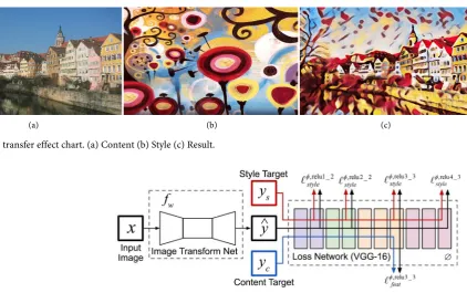
trained by SGD, and the effect diagram is shown in Figure 1.

The purpose is to calculate the weighted sum of a series of loss functions by operation, and the formula is:

{ }

(

( )

)

*

, 1

arg min ,

i i i W i

x y i

W = E _

∑

γ

We used a pre-trained network φ for image classification to define our loss function. We then train our deep convolutional transformation network using a

(a) (b) (c) Figure 1. Style transfer effect chart. (a) Content (b) Style (c) Result.

DOI: 10.4236/ojapps.2019.98053 666 Open Journal of Applied Sciences loss function that is also a deep convolutional network, as shown in Figure 2. The loss network φ is able to define a feature (content) loss lfeat and a style loss

lstyle, respectively measuring the difference in content and style. For each input

image x we have a content target yc a style target ys, for style conversion, the

content target yc is the input image x, the output image y, the style Ys should be

combined to the content x = yc. We train a network for each target style.

3.2.1. Construction of Image Conversion Network

Instead of any pooling layer, we use a convolution or micro-step convolution in-stead. Our neural network consists of five residual blocks. All non-residual con-volutional layers follow a spatial batch-normalization, and the nonlinear layer of the RELU, with the exception of the last output layer. The last layer uses a scaled Tanh to ensure that the pixels of the output image are between [0, 255]. Except for the first and last layers with a 9 × 9 kernel, all other convolutional layers use 3 × 3 kernels.

Input and Output: For style conversion, both input and output are color im-ages, size 3 × 256 × 256. For super-resolution reconstruction, there is an upsam-pling factor f, the output is a high resolution image 3 × 288 × 288, the input is a low resolution image 3 × 288/f × 288/f, because the image conversion network is com-pletely convolved, so during the test, it can be applied to images of any resolution.

Downsampling and Upsampling: For super-resolution reconstruction, there is an upsampling factor f, and we use several residual blocks followed by the Log2f volume and the network (stride = 1/2). This process is different from [1]. Double-cubic interpolation is used to upsample this low-resolution input before putting the input into the network. Without relying on any fixed upsampling interpolation function, the microstep convolution allows the upsampling func-tion to be trained along with the rest of the network. For image conversion, our network uses two contension = 2 convolutions to downsample the input, fol-lowed by several residual blocks, folfol-lowed by two convolution layers (stride = 1/2) upsampling.

3.2.2. Perceptual Loss Function

We define two perceptual loss functions to measure the high level of perceptual and semantic differences between two images. Use a pre-trained network model for image classification. In our experiments this model was VGG-16 [25], using Imagenet’s dataset for pre-training.

Feature (content) loss: We do not recommend pixel-by-pixel comparison, but use VGG to calculate the advanced feature (content) representation. This method is the same as the original style using VGG-19 [26] to extract style fea-tures. The formula is:

(

)

( )

( )

,

2 1

ˆ, ˆ

j

feat j j

j j j

l y y y y

C H W

∅ _{= ∅ − ∅}

(6)

DOI: 10.4236/ojapps.2019.98053 667 Open Journal of Applied Sciences from the target y), so we also want to punish style deviations: color, texture, common patterns, and so on. In order to achieve such an effect, Gatys et al.

proposed a loss function for the following style reconstruction. Let φj(x)

represent the jth layer of the network φ, and the input is x. The shape of the fea-ture map is Cj × Hj × Wj, and the definition matrix Gj(x) is Cj × Cj matrix

(cha-racteristic matrix). The elements are derived from the following formula:

( )

( )

( )

1 Hj Wj

j c c h w j h w c j h w c

j j j

G x x x

C H W

∅

′ =

∑ ∑

If we understand φj(x) as a feature of the Cj dimension, and the size of each

feature is Hj × Wj, then the left Gj(x) is proportional to the non-central

cova-riance of the Cjdimension. Each grid location can be used as a separate sample.

This can therefore capture which feature can drive other information. The gra-dient matrix can be calculated in a very funny time by adjusting the shape of φj(x) to a matrix ψ, the shape is Cj × HjWj, and then Gj(x) is ψψT/CjHjWj. The

loss of style reconstruction is well defined, even when the output and target have different sizes, because with the gradient matrix, the two will be adjusted to the same shape.

4. Main Results

4.1. Conditional Confrontation Network Model

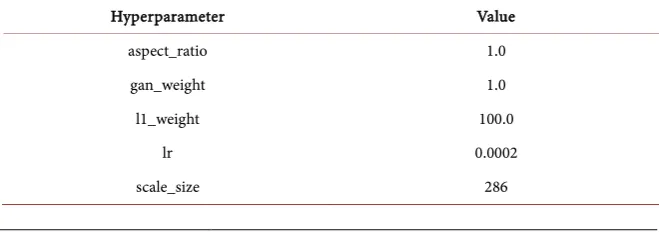
To optimize the versatility of GANs, we tested the method on a variety of tasks and data sets, including graphics tasks (such as photo generation) and visual tasks (such as semantic segmentation). We have found that very good results are often obtained on small data sets. The training data set we used contains only 400 images, and training can be made very fast with this size of training set. Some of the super parameters are shown in Table 1.

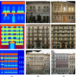
Qualitative results: the completed model is displayed, and the actual generated effect is displayed. Below we list three sets of pictures, as shown in Figure 3, the input of the figure, the second column is the output (model generation result), and the third column is the actual result. Equation (8) is the calculation formula used. A lot of experiments show that our average is around 0.4.

time rate

max_steps

= ₍₈₎

Table 1. Training hyperparameter selection and result numerical mapping ratio.

Hyperparameter Value

aspect_ratio 1.0

gan_weight 1.0

l1_weight 100.0

lr 0.0002

DOI: 10.4236/ojapps.2019.98053 668 Open Journal of Applied Sciences Figure 3. Conditional confrontation network model implementation rendering. (a) input (b) Model generation result (c) result.

4.2. Style Migration

The goal of style conversion is to produce a picture with both the content infor-mation of the content map and the style inforinfor-mation of the style map. As a base-line, we reproduce the method of Gatys et al., giving the style and content goals

ys and yc, layer i and J represent feature and style reconstruction. The

imple-mentation formula is:

(

)

(

)

( )

, ,

ˆ arg min , ,

TV

j j

c feat c s fstyle s TVl

y=

µ

µ

µ

In the formula, u starts with parameters, y is initialized to white noise, and is optimized with LBFGS. We found that unconstrained optimization equations usually cause the pixel values of the output image to go beyond [0, 255] to make a more fair comparison. For the baseline, we use L-BFGS projection, and adjust the image y to each iteration. [0, 255], in most cases, the computational optimi-zation converges to satisfactory results within 500 iterations, which is slower be-cause each LBFGS iteration requires feedforward feedback and feedback through the VGG16 network.

Training details: Our style conversion network is trained with COCO data-sets. We adjust each image to 256 × 256, a total of 80,000 training charts, batch-size = 4, iterations 40,000 times, and about two rounds. Optimized with

DOI: 10.4236/ojapps.2019.98053 669 Open Journal of Applied Sciences Adam, the initial learning rate is 0.001. The output graph is normalized by the whole variable (strength between 1e-6 and 1e-4), selected by cross-validation set. There is no weight attenuation or dropout because the model has no overfitting in these two rounds. For all style conversion experiments we take the relu2_2 layer for content, relu1_2, relu2_2, relu3_3 and relu4_3 as styles. For the VGG-16 network, our experiments used Torch and cuDNN, and the training took about 4 hours on a GTX Titan X GPU.

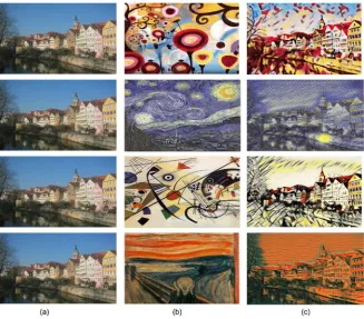
Qualitative results: For the model after training, we performed the actual ef-fect test. We screened out four sets of images, as shown in Figure 4. In the fig-ure, column a provides content features for content images, and column b pro-vides style textures for style images. We train different models to migrate effects for different styles. In column 4 of column 4, compared with the optimized me-thod, our network produces comparable quality results, but can achieve three orders of magnitude speed increase. This optimization is of great significance for practical applications. After a lot of experiments, the average time we took the picture was around 10 seconds.

4.3. Model Combination

We combine the conditional confrontation network model and the style transfer model to achieve a good combination effect. The specific results are shown in

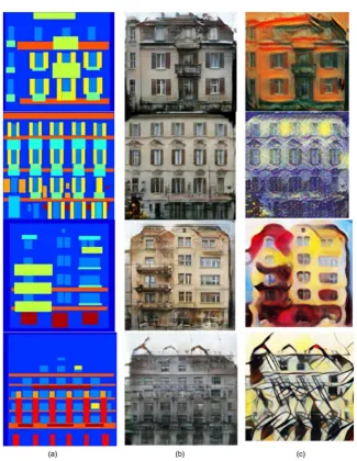
Figure 5. The a column is the sketch, the b column is the generated result, and the c column is the effect after the style transfer.

DOI: 10.4236/ojapps.2019.98053 670 Open Journal of Applied Sciences Figure 5. Schematic diagram of the results of the model. (a) input (b) output1 (c) out-put2.

5. Conclusion

DOI: 10.4236/ojapps.2019.98053 671 Open Journal of Applied Sciences of the image, achieve more realistic comic style migration effects, and imitate different painter strokes and for buildings and characters adapt to different pa-rameters.

Conflicts of Interest

The authors declare no conflicts of interest regarding the publication of this pa-per.

References

[1] Krizhevsky, A., Sutskever, I., Hinton, G.E., et al. (2012) ImageNet Classification with Deep Convolutional Neural Networks. Neural Information Processing Sys-tems, 141, 1097-1105.

[2] Zheng, S., Jayasumana, S., Romeraparedes, B., et al. (2015) Conditional Random Fields as Recurrent Neural Networks. International Conference on Computer Vi-sion, Santiago, 7-13 December 2015, 1529-1537.

https://doi.org/10.1109/ICCV.2015.179

[3] Long, J., Shelhamer, E., Darrell, T., et al. (2015) Fully Convolutional Networks for Semantic Segmentation. Computer Vision and Pattern Recognition, Boston, 7-12 June 2015, 3431-3440.https://doi.org/10.1109/CVPR.2015.7298965

[4] Noh, H., Hong, S., Han, B., et al. (2015) Learning Deconvolution Network for Se-mantic Segmentation. International Conference on Computer Vision, Santiago, 7-13 December 2015, 1520-1528.https://doi.org/10.1109/ICCV.2015.178

[5] Cheng, Z., Yang, Q., Sheng, B., et al. (2015) Deep Colorization. International Con-ference on Computer Vision, Santiago, 7-13 December 2015, 415-423.

https://doi.org/10.1109/ICCV.2015.55

[6] Dangelo, E., Alahi, A., Vandergheynst, P., et al. (2012) Beyond Bits: Reconstructing Images from Local Binary Descriptors. International Conference on Pattern Recog-nition, Tsukuba, Japan, 11-15 November 2012, 935-938.

[7] Vondrick, C., Khosla, A., Malisiewicz, T., et al. (2013) HOGgles: Visualizing Object Detection Features[C]. International Conference on Computer Vision, Sydney, 1-8 December 2013, 1-8.https://doi.org/10.1109/ICCV.2013.8

[8] Mahendran, A. and Vedaldi, A. (2015) Understanding Deep Image Representations by Inverting Them. Computer Vision and Pattern Recognition, Boston, 7-12 June 2015, 5188-5196.https://doi.org/10.1109/CVPR.2015.7299155

[9] Gatys, L.A., Ecker, A.S. and Bethge, M. (2015) Texture Synthesis Using Convolu-tional Neural Networks. In: Advances in Neural Information Processing Systems, Neural Information Processing Systems Foundation, Quebec, 262-270.

https://doi.org/10.1109/CVPR.2016.265

[10] Gatys, L.A., Ecker, A.S. and Bethge, M. (2015) A Neural Algorithm of Artistic Style. Computer Science, 11, 510-519.

[11] He, K., Zhang, X., Ren, S., et al. (2016) Deep Residual Learning for Image Recogni-tion. Computer Vision and Pattern Recognition, Las Vegas, 27-30 June 2016, 770-778.https://doi.org/10.1109/CVPR.2016.90

[12] Isola, P., Zhu, J., Zhou, T., et al. (2017) Image-to-Image Translation with Condi-tional Adversarial Networks. Computer Vision and Pattern Recognition, Honolulu, 21-26 July 2017, 5967-5976.https://doi.org/10.1109/CVPR.2017.632

Confe-DOI: 10.4236/ojapps.2019.98053 672 Open Journal of Applied Sciences rence on Computer Vision, Santiago, 7-13 December 2015, 1395-1403.

https://doi.org/10.1109/ICCV.2015.164

[14] Chen, L., Papandreou, G., Kokkinos, I., et al. (2015) Semantic Image Segmentation with Deep Convolutional Nets and Fully Connected CRFs. International Confe-rence on Learning Representations, San Diego, CA, 9 April 2015.

[15] Wang, Z., Bovik, A.C., Sheikh, H.R., et al. (2004) Image Quality Assessment: From Error Visibility to Structural Similarity. IEEE Transactions on Image Processing, 13, 600-612.https://doi.org/10.1109/TIP.2003.819861

[16] Dosovitskiy, A. and Brox, T. (2016) Generating Images with Perceptual Similarity Metrics Based on Deep Networks. Neural Information Processing Systems, Barce-lona, Spain, 5-10 December 2016, 658-666.

[17] Li, C. and Wand, M. (2016) Combining Markov Random Fields and Convolutional Neural Networks for Image Synthesis. Computer Vision and Pattern Recognition, Las Vegas, 27-30 June 2016, 2479-2486.https://doi.org/10.1109/CVPR.2016.272 [18] Xie, S., Huang, X., Tu, Z., et al. (2016) Top-Down Learning for Structured Labeling

with Convolutional Pseudoprior. European Conference on Computer Vision, Ams-terdam, 8-16 October 2016, 302-317.https://doi.org/10.1007/978-3-319-46493-0_19 [19] Johnson, J., Alahi, A., Feifei, L., et al. (2016) Perceptual Losses for Real-Time Style

Transfer and Super-Resolution. European Conference on Computer Vision, Ams-terdam, 8-16 October 2016, 694-711.https://doi.org/10.1007/978-3-319-46475-6_43 [20] Mirza, M. and Osindero, S. (2014) Conditional Generative Adversarial Nets. [21] Pathak, D., Krahenbuhl, P., Donahue, J., et al. (2016) Context Encoders: Feature

Learning by Inpainting. Computer Vision and Pattern Recognition, Las Vegas, 27-30 June 2016, 2536-2544.https://doi.org/10.1109/CVPR.2016.278

[22] Wang, X. and Gupta, A. (2016) Generative Image Modeling Using Style and Struc-ture Adversarial Networks. European Conference on Computer Vision, Amster-dam, 8-16 October 2016, 318-335.https://doi.org/10.1007/978-3-319-46493-0_20 [23] Yoo, D., Kim, N., Park, S., et al. (2016) Pixel-Level Domain Transfer. European

Conference on Computer Vision, Amsterdam, 8-16 October 2016, 517-532. https://doi.org/10.1007/978-3-319-46484-8_31

[24] Li, C. and Wand, M. (2016) Precomputed Real-Time Texture Synthesis with Mar-kovian Generative Adversarial Networks. European Conference on Computer Vi-sion, Amsterdam, 8-16 October 2016, 702-716.

https://doi.org/10.1007/978-3-319-46487-9_43

[25] Ronneberger, O., Fischer, P., Brox, T., et al. (2015) U-Net: Convolutional Networks for Biomedical Image Segmentation. Medical Image Computing and Computer As-sisted Intervention, Munich, 5-9 October 2015, 234-241.

https://doi.org/10.1007/978-3-319-24574-4_28