Bayesian Multi-Model
Frameworks
Properly Addressing Conceptual Uncertainty
in Applied Modelling
Dissertation
der Mathematisch-Naturwissenschaftlichen Fakult¨at der Eberhard Karls Universit¨at T¨ubingen
zur Erlangung des Grades eines Doktors der Naturwissenschaften
(Dr. rer. nat.) vorgelegt von
Marvin H¨
oge
aus M¨uhlacker T¨ubingen 2019Gedruckt mit Genehmigung der Mathematisch-Naturwissenschaftlichen Fakult¨at der Eberhard Karls Universit¨at T¨ubingen.
Tag der m¨undlichen Qualifikation: 25.2.2019
Dekan: Prof. Dr. Wolfgang Rosenstiel
1. Berichterstatter: Prof. Dr.-Ing. Olaf Cirpka 2. Berichterstatter: Prof. Dr.-Ing. Wolfgang Nowak 3. Berichterstatter: Dr. Thomas W¨ohling
Abstract
We use models to understand or predict a system. Often, there are multiple plausi-ble but competing model concepts. Hence, modelling is associated with conceptual uncertainty, i.e., the question about proper handling of such model alternatives. For mathematical models, it is possible to quantify their plausibility based on data and rate them accordingly. Bayesian probability calculus offers several for-mal multi-model frameworks to rate models in a finite set and to quantify their conceptual uncertainty as model weights. These frameworks are Bayesian model selection and averaging (BMS/BMA), Pseudo-BMS/BMA and Bayesian Stacking. The goal of this dissertation is to facilitate proper utilization of these Bayesian multi-model frameworks. They follow different principles in model rating, which is why derived model weights have to be interpreted differently, too. These prin-ciples always concern the model setting, i.e., how the models in the set relate to one another and the true model of the system that generated observed data. This relation is formalized in model scores that are used for model weighting within each framework. The scores resemble framework-specific compromises between the ability of a model to fit the data and the therefore required model complexity. Hence, first, the scores are investigated systematically regarding their respective take on model complexity and are allocated in a developed classification scheme. This shows that BMS/BMA always pursues to identify the true model in the set, that Pseudo-BMS/BMA searches the model with largest predictive power despite none of the models being the true one, and that, on that condition, Bayesian Stacking seeks reliability in prediction by combining predictive distributions of multiple models.
An application example with numerical models illustrates these behaviours and demonstrates which misinterpretations of model weights impend, if a certain fra-mework is applied despite being unsuitable for the underlying model setting. Re-garding applied modelling, first, a new setting is proposed that allows to identify a “quasi-true” model in a set. Second, Bayesian Bootstrapping is employed to take into account that rating of predictive capability is based on only limited data. To ensure that the Bayesian multi-model frameworks are employed properly and goal-oriented, a guideline is set up. With respect to a clearly defined modelling goal and the allocation of available models to the respective setting, it leads to the suitable multi-model framework. Aside of the three investigated frameworks, this guideline further contains an additional one that allows to identify a (quasi-)true model if it is composed of a linear combination of the model alternatives in the set.
The gained insights enable a broad range of users in science practice to properly employ Bayesian multi-model frameworks in order to quantify and handle con-ceptual uncertainty. Thus, maximum reliability in system understanding and pre-diction with multiple models can be achieved. Further, the insights pave the way for systematic model development and improvement.
Kurzfassung
Wir benutzen Modelle, um ein System zu verstehen oder vorherzusagen. Oft gibt es dabei mehrere plausible aber konkurrierende Modellkonzepte. Daher geht Model-lierung einher mit konzeptioneller Unsicherheit, also der Frage nach dem angemes-senen Umgang mit solchen Modellalternativen. Bei mathematischen Modellen ist es m¨oglich, die Plausibilit¨at jedes Modells anhand von Daten des Systems zu quan-tifizieren und Modelle entsprechend zu bewerten. Bayes’sche Wahrscheinlichkeits-rechnung bietet dazu verschiedene formale Multi-Modellrahmen, um Modellalter-nativen in einem endlichen Set zu bewerten und ihre konzeptionelle Unsicherheit als Modellgewichte zu beziffern. Diese Rahmen sind Bayes’sche Modellwahl und -mittelung (BMS/BMA), Pseudo-BMS/BMA und Bayes’sche Modellstapelung. Das Ziel dieser Dissertation ist es, den ad¨aquaten Umgang mit diesen Bayes’schen Multi-Modellrahmen zu erm¨oglichen. Sie folgen unterschiedlichen Prinzipien in der Modellbewertung weshalb die abgeleiteten Modellgewichte auch unterschiedlich zu interpretieren sind. Diese Prinzipien beziehen sich immer auf das Modellsetting, also darauf, wie sich die Modelle im Set zueinander und auf das wahre Modell des Systems beziehen, welches bereits gemessene Daten erzeugt hat. Dieser Bezug ist in Kenngr¨oßen formalisiert, die innerhalb jedes Rahmens der Modellgewichtung dienen. Die Kenngr¨oßen stellen rahmenspezifische Kompromisse dar, zwischen der F¨ahigkeit eines Modells die Daten zu treffen und der dazu ben¨otigten Modellkom-plexit¨at.
Daher werden die Kenngr¨oßen zun¨achst systematisch auf ihre jeweilige Bewertung von Modellkomplexit¨at untersucht und in einem entsprechend entwickelten Klas-sifikationschema zugeordnet. Dabei zeigt sich, dass BMS/BMA stets verfolgt das wahre Modell im Set zu identifizieren, dass Pseudo-BMS/BMA das Modell mit der h¨ochsten Vorsagekraft sucht, obwohl kein wahres Modell verf¨ugbar ist, und dass Bayes’sche Modellstapelung unter dieser Bedingung Verl¨asslichkeit von Vor-hersagen anstrebt, indem die Vorhersageverteilungen mehrerer Modelle kombiniert werden.
Ein Anwendungsbeispiel mit numerischen Modellen verdeutlicht diese Verhaltenwei-sen und zeigt auf, welche Fehlinterpretationen der Modellgewichte drohen, wenn ein bestimmter Rahmen angewandt wird, obwohl er nicht zum zugrundeliegen-den Modellsetting passt. Mit Bezug auf anwendungsorientierte Modellierung wird dabei erstens ein neues Setting vorgestellt, das es erm¨oglicht, ein “quasi-wahres” Modell in einem Set zu identifizieren. Zweitens wird Bayes’sches Bootstrapping eingesetzt um bei der Bewertung der Vorhersageg¨ute zu ber¨ucksichtigen, dass diese auf Basis weniger Daten erfolgt.
Um zu gew¨ahrleisten, dass die Bayes’schen Multi-Modellrahmen angemessen und zielf¨uhrend eingesetzt werden, wird schließlich ein Leitfaden erstellt. Anhand eines klar definierten Modellierungszieles und der Einordnung der gegebenen Modelle in das entspechende Setting leitet dieser zum geeigneten Multi-Modellrahmen. Ne-ben den drei untersuchten Rahmen enth¨alt dieser Leitfaden zudem einen weiteren, der es erm¨oglicht ein (quasi-)wahres Modell zu identifizieren, wenn dieses aus einer Linearkombination der Modellalternativen im Set besteht.
Die gewonnenen Erkenntnisse erm¨oglichen es einer breiten Anwenderschaft in Wis-senschaft und Praxis, Bayes’sche Multi-Modellrahmen zur Quantifizierung und Handhabung konzeptioneller Unsicherheit ad¨aquat einzusetzen. Dadurch l¨asst sich maximale Verl¨asslichkeit in Systemverst¨andis und -vorhersage durch mehrere Mo-delle erreichen. Die Erkenntnisse ebnen dar¨uber hinaus den Weg f¨ur systematische Modellentwicklung und -verbesserung.
Contents
List of Figures VIII
List of Tables IX List of Symbols X List of Acronyms XI 1 Introduction 1 1.1 Motivation . . . 1 1.2 This Thesis . . . 8
1.2.1 Goals and Objectives . . . 8
1.2.2 Research Questions and Contributions . . . 8
1.2.3 Thesis Structure . . . 10
2 Theory & Methods 11 2.1 Model Theory . . . 11
2.1.1 A Refined Model Definition . . . 11
2.1.2 Model Conceptuality: Model Types and Model Fidelity . . . 13
2.1.3 Mathematical Spaces covered by Modelling . . . 15
2.1.4 Model Space Settings . . . 16
2.2 Bayesian Inference and Uncertainty Quantification . . . 20
2.2.1 Uncertainty, Knowledge and Bayesian Priors . . . 20
2.2.2 Bayesian Model Inference . . . 22
2.2.3 Likelihood Function and Prediction Errors . . . 24
2.2.4 Scores and Divergences . . . 26
2.3 Bayesian Multi-Model Frameworks . . . 28
2.3.1 Bayesian Model Selection and Averaging . . . 29
2.3.2 Predictive (Bayesian) Model Selection and Averaging . . . . 32
2.3.3 Bayesian Stacking . . . 35
2.4 Implementation of Bayesian Inference . . . 37
2.4.1 Inferring Distributions and Normalizing Constants . . . 37
2.4.2 Bayesian Bootstrap . . . 39
2.5 Approximative Model Rating Methods . . . 41
2.5.1 B1: Posterior Model Probability . . . 42
2.5.2 B0: Code Length . . . 43
2.5.3 A1: Predictive Density . . . 45
3 Investigating the Role of Model Complexity in Model Rating and
Selection 52
3.1 Model Fit and Model Complexity . . . 52
3.1.1 Overfitting and Underfitting . . . 52
3.1.2 Model Complexity Control . . . 54
3.2 The Role of Model Complexity within Model Selection Criteria . . . 56
3.2.1 Consistency in Model Selection . . . 57
3.2.2 Bounds of Consistent Model Selection . . . 59
3.2.3 Bayesianism in Model Selection . . . 60
3.2.4 The Role of Priors in Model Selection . . . 62
3.3 Classification of Model Selection Criteria . . . 63
3.3.1 Classification Scheme . . . 63
3.3.2 Contrasting the Views on Models and their Complexity . . . 65
3.3.3 Matching Model Selection Classes with Model Types . . . . 67
3.3.4 Alternative Model Selection Criteria . . . 68
3.4 Cross-Comparison between Model Selection Criteria . . . 69
3.4.1 B1- vs. B0-type Criteria . . . 69
3.4.2 A1- vs. A0-type Criteria . . . 70
3.4.3 A-type vs. B-type: Large Sample Limit . . . 71
3.4.4 Model Selection by AIC and BIC Exemplified . . . 72
3.5 Summary and Conclusion . . . 75
4 Applying Bayesian Multi-Model Frameworks Properly to Model Settings 78 4.1 Modelling Task, Data and Models . . . 78
4.1.1 Lab-scale Experiment, Data and Likelihood Function . . . . 79
4.1.2 Mechanistic models . . . 80
4.1.3 Summary of the Reference Study . . . 81
4.2 Conducting Bayesian Multi-Model Inference . . . 84
4.2.1 Defining a Quasi-M-closed setting . . . 84
4.2.2 Evaluating Multi-Model Frameworks in Different M-settings 85 4.2.3 Obtaining the Marginalized Likelihoods . . . 87
4.3 Results and Discussion . . . 89
4.3.1 Model Weights in the M-closed Setting . . . 89
4.3.2 Model Weights in the Quasi-M-closed Setting . . . 90
4.3.3 Model Weights in the M-complete Setting . . . 92
4.3.4 Validation in Quasi-M-closed andM-complete settings . . . 94
5 Guiding toward Task-Specific Multi-Model Use 100
5.1 Disentangling Model Combination Terminology . . . 100
5.2 Bayesian Model Combination for Process Identification . . . 101
5.3 Averaging of Model Outputs vs. Predictive Distributions . . . 104
5.4 Guideline to Identify the Best-Suited Multi-Model Approach . . . . 106
5.5 Summary, Discussion and Conclusion . . . 107
6 Conclusion & Outlook 109 A Numerical Methods for Bayesian Inference 115 A.1 Importance Sampling . . . 115
A.2 Power-Posterior and Thermodynamic Integration . . . 120
A.2.1 Power-Posterior Distributions . . . 120
A.2.2 Thermodynamic Integration . . . 120
A.2.3 Related “Tempered” Methods . . . 122
A.3 Alternative Methods . . . 122
A.4 Numerical Techniques . . . 123
A.5 Available Software . . . 124
B Applied Model Complexity Control 126 B.1 Model Complexity within Selection Criteria: Synthetic Example . . 126
B.1.1 Numerical Implementation . . . 126
B.1.2 B-type Model Complexity . . . 128
B.1.3 A-type Model Complexity . . . 129
B.2 Complexity Control in Black-Box Models . . . 130
C Analytic Solutions to Marginalized Likelihoods: Gaussian Linear
List of Figures
1 Model conceptuality: model type and model fidelity . . . 14
2 Illustration of M-settings: M-closed, M-complete and M-open . . 17
3 Illustration of Bayesian inference . . . 23
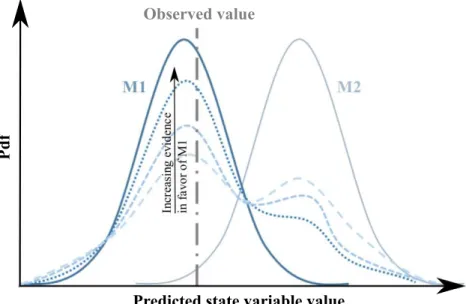
4 Predictive pdf from BMS/BMA . . . 31
5 Concepts and effects of bias and variance . . . 53
6 Illustrated underfitting and overfitting . . . 53
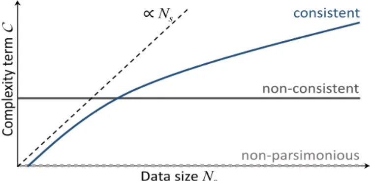
7 Schematic behaviour complexity termsC within model selection cri-teria . . . 56
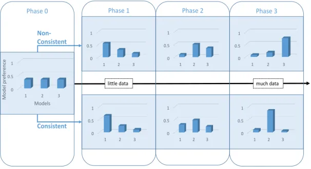
8 Model rating example: Differences in model rating following non-consistent (A-type) and non-consistent (B-type) model selection . . . 58
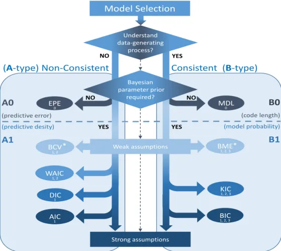
9 Principle classification system for model selection methods . . . 62
10 Filled classification system for model selection methods . . . 64
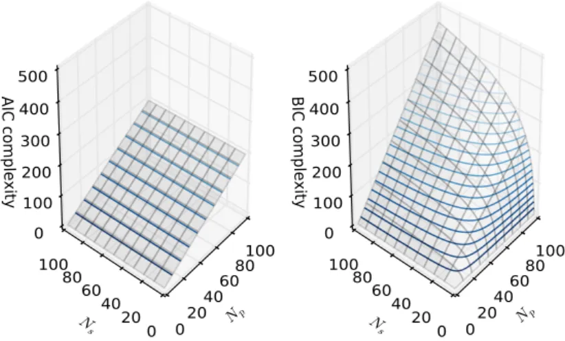
11 Model complexity representation of AIC and BIC over numbers of parameters and observations . . . 71
12 Neural network classification example: Models and data . . . 72
13 Neural network classification example: Maximum likelihood results 73 14 Neural network classification example: Model weights via AIC and BIC . . . 74
15 Laboratory sandbox aquifer: photograph and models . . . 80
16 Illustration ofM-settings: M-closed, Quasi-M-closed,M-complete and M-open . . . 85
17 Defined M-settings for the applied modelling example . . . 86
18 Expected model weights in theM-closed setting . . . 89
19 Expected model weights in the Quasi-M-closed setting . . . 91
20 Expected model weights in theM-complete setting . . . 93
21 Contrasting BMS/BMA and BCMS/BCMA . . . 103
22 Guideline to the most suitable Bayesian multi-model framework . . 106
23 Illustrated importance sampling . . . 115
24 Scheme of Parallel Tempering MCMC . . . 124
25 Selected consistent complexity measures evaluated over growing data size . . . 128
26 Selected non-consistent complexity measures evaluated over growing data size . . . 129
List of Tables
1 Summary ofM-settings: M-closed, M-complete and M-open . . . 18 2 Examples of conjugate distributions . . . 38 3 Class-specific consideration of models and their complexity . . . 66 4 Predictive performance of individual models . . . 83 5 Summary of M-settings: M-closed, Quasi-M-closed, M-complete
and M-open . . . 85 6 Predictive performance of model averages in the Quasi-M-closed
setting . . . 95 7 Predictive performance of model averages in theM-complete setting 96 8 Contrasting summary of BMS/BMA vs. Pseudo-BMS/BMA . . . . 119 9 Sophisticated MCMC techniques . . . 123 10 DGP and models for evaluating model complexity measures . . . . 126
List of Symbols
p(·) andq(·) Marginal (prior) probability density function of a random variable
p(·|·) Conditional (posterior) probability density function of a random variable E[·] or E[·|·] Expectation of a random variable (marginal or conditional)
Var[·] or Var[·|·] Variance of a random variable (marginal or conditional)
D Within-sample/calibration data vector D0 Out-of-sample/validation data vector Measurement error vector
Θ Model parameter vector from parameter space Ωm
x Model input vector
y Model prediction/forecast/output vector from prediction space Y
ˆ
y Best estimate (e.g., maximum likelihood) model prediction vector
Mm Individual model m from model space M
M Model set / ensemble
wm Model weight of model m
w Model weight vector
Ns Number of observations Np Number of parameters
Np∗ Number of effective parameters
NM Number of models
S Model rating score
F Goodness-of-fit term
C Model Complexity term
K Convex set of models
ln(·) natural logarithm
List of Acronyms
BB Bayesian Bootstrap
BCMS/BCMA Bayesian combined model selection / averaging BCV Bayesian cross-validation
BME Bayesian model evidence
BMS/BMA Bayesian model selection / averaging DGP Data-generating process
DKL Kullback-Leibler divergence
DoF Degrees of freedom
elpd Expected logarithmic predictive density EPE Expected prediction error
GC Geometric complexity
i.i.d. Independent and identically distributed LOO (CV) Leave-one-out (cross-validation)
MC Monte Carlo
MCMC Markov Chain Monte Carlo MDL Minimum Description Length
OF Occam factor
PDE Partial differential equation pdf Probability density function
Pseudo-BMS/BMA Pseudo-Bayesian model selection / averaging QoI Quantity of interest
RMSE root-mean-square error
WSSE weighted sum of squared errors
1
Introduction
1.1
Motivation
Models and Uncertainty in Modelling
Whenever we want an explanation of the past, confirmation in the present or predictions of the future, we employ models. In most simple and general terms, a model is “a thing used as an example to follow or imitate” (Oxford), i.e., something that allows us to understand or forecast behaviour of the system we are interested in, whether its underlying relations are of physical, ecological, technical, political, social, economical, financial, or other nature. More specifically, for quantitative modelling of systems, models are rather to interpret as “a simplified description, especially a mathematical one, of a system or process, to assist calculations and predictions” (Oxford). Mathematical models enable us to simulate systems under all kinds of conditions, to perform scenario analyses and, ultimately, to support decision-making (Reichert et al., 2015; Ferr´e, 2017).
However, modelling is subject to uncertainty. The shear attempt of creating a model implies uncertainty due to simplifications, assumptions, etc. Operating a model adds and propagates uncertainty further due to all kinds of errors, vague included observations, etc. Therefore, modelling comes with an intrinsic demand for uncertainty quantification. Numerous approaches were proposed about how to quantify uncertainty in model results based of sensitivity analyses (Gupta and Razavi, 2018), interval computation (Moore, 1979), fuzzy set theory (Zadeh, 1965; Klir and Yuan, 1995) and possibility theory (Zadeh, 1999) or entropy (Shannon, 1948), naming just a few. Yet, the most thoroughly discussed and widely used tool to quantify uncertainty is probability theory (Gillies, 2012).
In particular, Bayesian inference proved to be suitable to handle uncertainty be-cause under the Bayesian paradigm probability resembles belief that quantifies lack of knowledge (e.g. Bernardo and Smith, 1994; Gelman and Shalizi, 2013), i.e., the paramount origin of uncertainty in modelling. Under this interpretation, Bay-esian probability theory remains as the only consistent mathematical calculus for uncertainty quantification (Nearing et al., 2016, and references therein). Plainly, mathematical models contain parameters that map a certain input to a correspon-ding output. Bayesian inference provides a comprehensive framework that allows to address the vague notion of overall model uncertainty, e.g., by decomposing it accordingly into parameter, input, output and so-called conceptual uncertainty (Renard et al., 2010; Sch¨oniger et al., 2014).
Multiple Models and Conceptual Uncertainty
While parameter, input and output uncertainty are evaluated for individual mo-dels, they can be subsumed under the overarching conceptual uncertainty, i.e., the question of how to deal with multiple alternative models (hypotheses). This un-certainty goes beyond how the parameters can map input to output more reliably
to whether the chosen parametrization is adequate at all. It defines which inputs, parameters and outputs are relevant and targets at the very core of science: sys-tematic hypothesis testing and inductive inference, i.e., how to infer general rules from special cases and observations (Rathmanner and Hutter, 2011).
This issue about model choice dates back to ancient philosophy where Epicurus stated the principle of multiple explanations and, concomitant, to never discard a plausible hypothesis when it is consistent with the observations (e.g. Rathmanner and Hutter, 2011). The multi-model approach stands to reason also in light of the Duhem-Quine thesis (see Harding, 1975), i.e., that any single model suffers from underdetermination by observations. Thereafter, a single hypothesis cannot be isolated and evaluated because it always relies on other (auxiliary) hypotheses or assumptions. Hence, multiple models that utilize divergent auxiliaries illuminate a system from different angles and thereby shed light on shortcomings of individual models.
Employing multiple models requires rules to rate their ability to “follow or imitate” to the modelers desire. Some models are more plausible than others and objective model rating prevents us from unreasonable preference of one model over others (Elliott and Brook, 2007). However, a rationale for such rules and formal rating is not straight-forward. A qualitative heuristic is given by Occam’s razor (e.g. Hut-ter, 2007, and references therein). It states that between competing hypotheses, the model that needs fewest assumptions (is the simplest model) while still being consistent with the observations is best. A model that follows this principle is called parsimonious (Angluin and Smith, 1983).
In our era of machine-based computation, Solomonoff (1964) formalized these prin-ciples for the first time entirely by a concept called algorithmic probability (Rath-manner and Hutter, 2011). The basic assumption is that our observations were generated by some “true” algorithm. In theory, it is then possible to systematically rate (Occam’s razor) all imaginable hypotheses (principle of multiple explanati-ons) by writing them down as algorithms and computing them on a Universal Turing Machine (Rathmanner and Hutter, 2011), i.e., the most general platform for algorithm execution (Gr¨unwald and Vit´anyi, 2003). Solomonoff’s algorithmic probability then allows to translate the code-length of each algorithm into a
Bay-esian probability. This way, it offers (theoretically) a way to place a probability distribution over the entirety of potential models (Hutter, 2007). Each algorithm resembles a compression of the observations - storing each observation separately resembles the longest possible code. Hence, the probability of an algorithm to be the optimal compression is the higher the shorter its code-length is. The best model, in this spirit, is the shortest code that can fully reproduce the observations and then halts (Gr¨unwald and Vit´anyi, 2003) - and this is the true data-generating algorithm. This comprehensive approach is called universal induction. It is the-oretically complete, but practically incomputable (Rathmanner and Hutter, 2011). Despite its practical inapplicability, the above concept sheds light on all issues of conceptual uncertainty in practice. Three principal issues and their consequences can be elicited:
1. The range of possible models is huge or even infinite - in theory, we need to check all alternatives to know which one is absolutely the best. In practice, we deal with a subset which is known asfinite hypotheses problem (Nearing et al., 2016). Therefore, it is by no means guaranteed, that one of our models is the algorithm that generated the data at all. Hence, we need a system to qualitatively describe the relation of this finite subset toward the so-called data generating process (DGP).
2. In scenarios where a true model of the DGP is unavailable, aiming at identi-fying it is no suitable objective. Then, conceptual uncertainty does not relate to the probability of being the true model any more. As a consequence the-reof, interpretations of conceptual uncertainty within such scenarios have to be adjusted. Subsequently, Occam’s razor for model rating and selection also needs to be realized by different means than algorithmic probability because the underlying assumptions are different, too.
3. Under the assumption that a true model cannot be found, it is questionable whether model rating with the ultimate goal to select only one model is promising. Rather, we require systematic approaches to successfully operate multiple non-true models.
In practice, we frequently consider multiple model alternatives (Clyde and Iversen, 2013) and therefore need guidance for appropriately matching “truth scenarios” and “razor implementations” in order to adequately rate and utilize a single mem-ber or multiple alternatives within a model set. Such guidance, however, is too rare and too little systematic in the available literature.
Model Types and Model Settings
For every modelling task at hand, it is typically possible to come up with several hypotheses that are consistent with the observations - theoretically, it is even “pos-sible to propose an infinite number of different models that allow us to correctly predict any finite number of events” (Nearing et al., 2016) if we had infinite time. Looking only at some model classification approaches reveals that numerous types of models and kinds of modelling schools exist: physics-based vs. data-driven, linear vs. non-linear, deterministic vs. stochastic, slow vs. fast, etc. (see, e.g., Refsgaard and Abbott, 1996; Breiman, 2001). Models fall into several of such ca-tegories, e.g., physics-based and stochastic, and even within such a specification there are countless possible alternatives. Using expert knowledge, we are able to restrict this huge variety but still, we can often only guess whether we “get close” to the DGP with a certain model or not.
Settings that describe whether (a) the true model is within our set of candidate models, (b) the true model exists but is outside of our set or (c) the true model is per se unavailable have been proposed by Bernardo and Smith (1994) from a decision theoretic perspective. They enable us to formalize this issue and serve as starting point for any kind of successive model rating. Despite the difficulty of transferring such settings to practical modelling tasks, such a distinction is crucial before any method for model rating can be applied: Model rating methods that are tailored to identify a true model will yield misleading results if applied in a setting where the true model is not included. Likewise, model rating methods that assume the truth to be unavailable among the candidate models can also never support the claim that the model they rate best is probably the true model. As example, when models are used to gain understanding of an isolated process in natural sciences they need to represent the relevant physics at the process-scale and have to be rated by methods that can identify a true model.
Mostly, such settings are recognized and discussed in the field of statistics (e.g. Clyde and Iversen, 2013). This motivates to elaborate on their relation to specific model types in order to make them accessible to a broader audience for practical application in other fields. Existing literature on model rating in most scientific disciplines does not take these settings into account.
Model Complexity and Model Rating
In practice, we typically deal with a finite set of distinct and fully defined models that share at least one objective like a quantity of interest (QoI) and account for conceptual uncertainty between all competitors in this respect. The law of
par-simony manifests itself as trade-off between quantified fit of model predictions to observations and the vague notion of model complexity: A model is best if it fits observations at least equally well or better while being simpler than the alterna-tive models. This implies that, for a given amount of data, there is an optimal complexity of a model (Claeskens, 2016), which is neither too complex, nor too simple (see Occam’s razor).
Numerous model rating methods were developed that all employ this trade-off but deviate vastly in their rating results due to the vagueness about what model complexity actually is. Universal induction (Solomonoff, 1964) provided the first rigorous definition of model complexity. Model rating methods that are directly derived from it link model complexity to code length (Gr¨unwald and Vit´anyi, 2003). Others measure model complexity by the number of (effective) parameters (Akaike, 1973; Spiegelhalter et al., 2002), the probabilistic distribution of para-meters (Kashyap, 1982), the sensitivity of parapara-meters to observations (Mallows, 1973), the spread of predictions (Friedman et al., 2001), mixtures of the previous or other means. There is no unique definition of model complexity and, often enough, model rating is only based on quantified fit obtained via an error metric like simple root-mean-square-error or so-called loss-functions without any conside-ration of model complexity. This is however insufficient regarding so-called model generalizability (e.g., Friedman et al., 2001), i.e., it does not allow to estimate the model performance for new data.
Among all those model rating methods, there are some that share the same un-derlying principles including similar representations of model complexity. Their asymptotic equality is often shown in the limit of infinite observations. However, in practice, there is only a limited amount of data. This limitation prevents that any hypothesis could ever be proven right (Popper, 2005; Tarantola, 2006) and exacerbates to assess which ones are good or bad (Nearing et al., 2016). Hence, the model rating methods require classification and interpretation with respect to the finite amount of data they are operated with and how they decide which mo-dels are better or worse than others. Attempts in this direction were made before (e.g. Kadane and Lazar, 2004; Yang, 2005; Vrieze, 2012), but are spread over many different scientific disciplines and typically compare distinct methods rather than aiming for an encompassing overview. A general classification scheme that, first, clearly depicts what is meant by model complexity, and, second, from which recommendations for action can be deduced for a specific modelling task at hand, is still missing.
Multi-model frameworks and their adequate utilization
Several multi-model frameworks are related to these model rating methods and allow for statistical model selection and averaging (e.g. Burnham and Anderson, 2004; Gelman et al., 2004). The most prominent example might be Bayesian Model Selection or Averaging (BMS or BMA; Draper, 1995; Hoeting et al., 1999; Raftery et al., 2005) in which model probabilities are used to express uncertainty between models in terms of how likely it is that a certain candidate model generated the observed data. Both BMS and BMA enjoy wide-spread usage over many disci-plines (e.g. Trotta, 2008; Faust et al., 2013; Hooten and Hobbs, 2015; Sch¨oniger, 2016) where they are often first choice to deal with conceptual uncertainty. Si-milarly, so-called Pseudo-BMA (Geisser and Eddy, 1979; Yao et al., 2017) is used to handle uncertainty between multiple models with respect to their individual ability to predict potential future data. In a similar spirit, model rating methods like the famous Akaike information criterion (AIC; Akaike, 1973, 1974) serve as basis for model selection. Other frameworks like (Bayesian) Stacking (Yao et al., 2017; Le et al., 2017) allow to combine model competitors in a set for predictive purposes rather than quantifying the uncertainty about one being relatively best. Despite the popularity of multi-model frameworks, their applications frequently cause confusion: different model selection criteria rate completely different models as “best” (Burnham and Anderson, 2002; Claeskens et al., 2008); despite a true model possibly being in the set, criteria like the AIC are not able to identify it (Vrieze, 2012); model averaging by BMA often yields worse predictive results than single model use (Domingos, 2000; Clarke, 2003), which raises the question whet-her model combination as weighted average can be provided by BMA at all (see Minka, 2002) and how actual model combination can successfully be performed (Clyde and Iversen, 2013; Le et al., 2017).
All of these problems can be traced back to the central question: Which multi-model framework employs the adequate Occam’s razor with respect to the multi-model setting of the modelling task at hand? Then, among other insights, it becomes apparent that “BMA is no panacea” (Clyde and Iversen, 2013) and that concep-tual uncertainty has different meanings and needs to be accounted for differently as well. Still, much too often the fundamental principles are neglected and multi-model methods are applied to practical multi-modelling tasks decoupled from them. A thorough investigation on these principles that collects insights from various scien-tific disciplines and elicits guidance by highlighting linkages to method application is still missing.
Water and Hydrosystem Modelling
While the philosophical and statistical questions of conceptual uncertainty concern all scientific disciplines on a rather abstract level, their answers pertain to very practical consequences when applied in fields with direct impact on our every-day lives. In hydrosystem modelling, our interest is water and its ubiquitous impact: life rests on the availability of water; we humans depend on it for drinking and agri-cultural irrigation, hygiene and health care, or energy and industrial production. Water is vital to us and our cultural progress and requires sustainable management of water quality and quantity. At the same time, the excessive abundance of water during floods or harmful scarcity of water throughout droughts in the course of weather and climate-related events require prognoses and adaption. Hydrosystem models help us to deal with these issues on distribution and protection of water resources and the risk assessment of water-related threats.
Traditionally, hydro(geo)logists employ process-based models (Freeze and Harlan, 1969; Montanari and Koutsoyiannis, 2012) to gain system understanding and as primary choice to support decision making (Reichert et al., 2015) in addressing the above challenges. Thereby, a major concern is uncertainty that arises from simpli-fication of the underlying physical processes (e.g. Renard et al., 2010; Clark et al., 2011; Refsgaard et al., 2012; Elshall and Tsai, 2014), which makes model com-plexity also a question of scale like temporal resolution or spatial variability and heterogeneity (Mendoza et al., 2015; Orth et al., 2015). As a consequence thereof the space of potential models expands by, e.g., lumped bucket-type (Bergstr¨om and Singh, 1995), spatially distributed (Refsgaard and Abbott, 1996), meso-scale hydrologic (Samaniego et al., 2010) models or even neural networks (Hsu et al., 1995) as modelling approaches on a completely different conceptual basis.
For decades, the hydro(geo)logic community has actively debated whether one ap-proach is more suitable than others (e.g. Freeze and Harlan, 1969; Bergstr¨om and Singh, 1995; Bl¨oschl and Sivapalan, 1995; Wagener et al., 2009; Mendoza et al., 2015). However, beyond individual preferences, there is no clear consensus on preferring one modelling approach over another when all approaches appear plau-sible for a certain task - and it remains questionable whether such a principle preference is justifiable. Nonetheless, there is consensus about the necessity to rigorously evaluate and rate models on a quantitative basis in order to justify an objective preference (e.g. Clark et al., 2008; Sch¨oniger et al., 2014). Correspon-dingly, the growing insight of the community that “stochastification” of models allows for rigorous estimation of uncertainty for all kinds of hydrosystem models (Liu and Gupta, 2007; de Barros and Nowak, 2010; Cirpka et al.; Montanari and Koutsoyiannis, 2012; Nearing et al., 2016) spurred various attempts of so-called
Bayesian total error analyses (Kavetski et al., 2006; Vrugt et al., 2008; Reichert and Mieleitner, 2009; Renard et al., 2010; Montanari and Koutsoyiannis, 2012; Giudice et al., 2013) up to the level of conceptual uncertainty estimation using, e.g., BMA (Ye et al., 2010; W¨ohling et al., 2015; Sch¨oniger, 2016) or AIC-related model rating (Schoups et al., 2008). Thereby, however, the same shortcomings of model selection and averaging methods as mentioned above have been recognized (e.g. Poeter and Anderson, 2005; Ye et al., 2008; Lu et al., 2011; Sch¨oniger, 2016).
1.2
This Thesis
1.2.1 Goals and Objectives
The goal of this thesis is to enable modellers to properly address conceptual un-certainty: For modelling tasks where multiple competing models are available, I explain and discuss which multi-model framework is most suitable to achieve a cer-tain modelling goal that complies with the underlying model setting. Therefore, I deeply analyse theoretical underpinnings of these frameworks; I demonstrate their proper usage in applied modelling; I unify scattered insights from across various scientific disciplines that work on related topics; and I offer a map for the confu-sing field of conceptual uncertainty. Ultimately, I aim at making these multi-model frameworks more accessible, in particular to applied modellers that often face con-ceptual uncertainty in practice but are not (yet) familiar with the background required to address it.
Bayesian multi-model frameworks allow for proper uncertainty quantification in stochastic modelling. Within this thesis, I clarify how these Bayesian tools work and how they can be used successfully when modellers desire process-identification, predictive reliability and decision support in multi-model use.
This thesis is an attempt to close the highlighted gaps in Section 1.1 by bridging the theoretical and philosophical underpinnings of multi-model usage to applied modelling tasks. Therefore, I focus on examples from hydrosystem modelling but, without any loss of generality, the insights can be transferred to other disciplines where models are used, e.g., machine learning, psychology, ecology, engineering or economics.
1.2.2 Research Questions and Contributions
An effective utilization of model rating methods and built-on multi-model frame-works is complicated by the sprawling amount of alternatives and lack of guidance. Modellers are often forced to pick one method in order to put model selection or
averaging on a quantifiable basis - often this is a commonly used one within the own scientific discipline. Yet, they have to rely on the chosen method to properly address conceptual uncertainty and have to trust the obtained model rating - often without fully knowing under which premisses the models are rated.
In order to establish guidance in this field, I want to invert this pattern by answe-ring the following research questions (RQ):
1. How is the law of parsimony implemented in different model rating and selection methods and what does this tell us about the evaluated models? 2. How are related multi-model frameworks properly used in specific modelling
settings and how are their often contradictory results interpreted correctly? 3. How can a multi-model framework be chosen for anymodelling task at hand such that the chosen framework properly addresses conceptual uncertainty specifically for this task?
These three research questions focus on different but complementary parts of the central question from Section 1.1: “Which multi-model framework employs the adequate Occam’s razor with respect to the model setting of the modelling task at hand?”
To answer the first RQ, I collected various model rating and selection methods that were developed and used over the last decades and dissected them with respect to their interpretation of model complexity, i.e., their implementation of Occam’s razor. Thereby, I merged insights about model selection from vastly different scien-tific disciplines and transferred them to applied modelling. As result, I developed a classification scheme for model selection criteria that allows to rate models ac-cording to whether a true model of an underlying DGP shall either be identified or only approached in an either Bayesian or non-Bayesian way. For each class, I discuss examples from hydrosystem modelling and propose matchings between certain modelling goals and model selection methods.
To answer the second RQ, I applied three Bayesian multi-model frameworks (BMA, Pseudo-BMA and Bayesian Stacking) to a finite model set for a typical task in hyd-rosystem modelling. Using the insights about the Occam’s razor implementations in my classification scheme from RQ 1, I analysed and contrasted how the three frameworks account for conceptual uncertainty in philosophically different model settings (see (a), (b) and (c) in Section 1.1). Therefore, additionally, I propose a new practical model setting (called Quasi-M-closed) to close a gap between the
existing ones for applied modelling. To assure reliability of the model rating re-sults within the frameworks, I further applied the so-called Bayesian Bootstrap method. This method allows to address insufficiently confident model ratings of predictive performance in case of using only a small amount of available data. By this practical example, I link the rigorous evaluation of Bayesian multi-model fra-meworks with specified model settings and the usage of Bayesian Bootstrapping in the context of hydrosystem modelling. Thereby, I demonstrate how the Bayesian multi-model frameworks are adequately employed to achieve process-identification or predictive reliability.
To answer the third RQ, I clarify which Bayesian multi-model frameworks allow for model combination for either identifying or approaching a true model - similarly to the different kinds of model selection from RQ 1. Therefore, I introduce a recent approach that merges these principles by selecting the best model combination for process-identification and exemplify it for a potential hydrosystem modelling task. In direct relation to the three Bayesian multi-model frameworks from RQ 2, I propose a guiding scheme that allows to find the appropriate multi-model framework for an arbitrary modelling task at hand. The guide shows that choosing a proper multi-modelling framework is the natural outcome when starting from the philosophical perspective on the modelling task, rather than picking one based on some ad-hoc preference.
1.2.3 Thesis Structure
This thesis is structured as follows: First, I introduce the underlying theory on models and model settings, as well as state-of-the-art Bayesian multi-model infe-rence methods in Chapter 2. Second, in three core chapters, I answer and discuss the three posed research questions:
• In Chapter 3, I answer RQ 1 and elucidate why some model selection criteria look similar but pursue vastly different goals of modelling. Thereby, the keyword is model complexity.
• In Chapter 4, I answer RQ 2 and demonstrate why respective model ra-ting results seem to mean the same but represent vastly different takes on conceptual uncertainty. Thereby, the keyword is model setting.
• In Chapter 5, I answer RQ 3 and elaborate why some multi-model frame-works have similar names but apply to vastly different modelling situations. Thereby, the keyword is model task.
Third and finally, I deduce conclusions from the found answers and discuss poten-tial issues for future research in Chapter 6.
2
Theory & Methods
Systematically addressing conceptual uncertainty requires a thorough considera-tion of model theory. Hence, I focus on model conceptuality and model settings in Section 2.1, on the principles behind Bayesian inference and uncertainty quantifi-cation in Section 2.2, on available Bayesian multi-model frameworks in Section 2.3, on their practical implementation in Section 2.4 and on common approximative methods for model rating in Section 2.5.
2.1
Model Theory
2.1.1 A Refined Model Definition
The previous chapter introduced two definitions of a model as “a thing used as an example to follow or imitate” or “a simplified description, especially a mathe-matical one, of a system or process, to assist calculations and predictions”. Both are kept as general definition that, in the spirit of Cartwright (1983), considers a model as a tool to translate a set of hypotheses and/or theories into predictions (e.g. Nearing et al., 2016). In order to translate this into mathematical terms, we define a model here as: mathematical function of interrelated parameters Θ
that map a certain input x to an output y while being subject to noise/error . The model parameters comprise latent variables ω like system properties and the “model frame” of boundary and initial conditions Γ (Θ={ω,Γbound,Γinit}):
Mm :y=f(x,Θ) + (1)
The above formulation for a model can most easily be understood as deterministic model, where all model parametersΘare fixed. Then, a certain input ˆxgenerates one specific f(ˆx) which equals the model output if is zero. Probabilistic models or deterministic models that are operated in a “stochastic framework” account for uncertainty of the components, e.g., specified by a probability distribution or pro-bability density function (pdf) over parameters p(Θ), input p(x) and noise p(). This results in a pdf of the model outputp(y). Therefore, stochastic modelling can be considered as generalization because taking the expectation over the assigned distributions yields a deterministic model.
A model set or model ensemble M refers to a finite list of NM models that are
fully specified and share at least one identical objective or QoI as output variable:
Despite its simplicity, the above definition of a modelMm as a thing to follow or
imitate essentially spans the entire spectrum of model types when we specify what
follow orimitate mean in the extremes (see, e.g., Breiman, 2001):
• follow refers to mechanistic modelling, where causal relations represent the modelled system. Mechanistic models help to understand and explain a sy-stem and allow for predictions based on causality. Universal natural laws and principles are specified for a certain system in a top-down manner. Physics-based models are an obvious example for mechanistic models and are often used synonymously. In hydro-system modelling, such a model would be the solution for the hydraulic head h as a function in space and time to the un-derlying parabolic partial differential equation (PDE) for groundwater flow:
S0
∂h
∂t − ∇(K∇h) = Qin/out (2)
with time t and ∇ as vector operator of partial derivatives in all spatial di-mensions, parameters storage coefficient S0 and hydraulic conductivity ten-sor K, state variable hydraulic head h, and sources and sinks term Qin/out
as boundary condition. Further, to specifically solve this mechanistic model, initial conditions likeh0 =h(t0) and boundary conditions like constant head or flux in space are required. Under steady-state conditions, the storage term in the groundwater flow equation drops out, turning the parabolic into an elliptic PDE −∇(K∇h) =Qin/out. Both contain the most fundamental law
in hydrogeology as example for the physical flux-gradient relationship, i.e., Darcy’s law for specific discharge q=−K∇h.
• imitate refers to data-driven modelling, where associations of system varia-bles are not necessarily causal. Data-driven models mimic a system and allow for predictions based on association of variables like correlation, regardless of whether there is causality or not. Patterns in the data are generalized for the observed or a similar system, i.e., a bottom-up approach. Empirical relations are exemplary for data-driven models, like a neural network (NN):
f(x) = ψ(W x+b) +b0 (3) A basic NN consists of interconnected nodes that allow for a non-linear map-ping. Mathematically, in its core, it is a simple linear matrix multiplication
of parameters known as weightsW between connected nodes and the vector of independent input variables x. A linear offset parameterb represents the bias at each node and b0 additionally adjusts for the bias of the NN out-put. The so-called activation function ψ(·) (typically a sigmoidal function) introduces non-linearity and allows the NN with its linear core to fit also non-linear data. A typical example from hydrosystem modelling is the pre-diction of non-linear stream discharge as output based on inputs like rainfall, evaporation, stored water, etc.
2.1.2 Model Conceptuality: Model Types and Model Fidelity
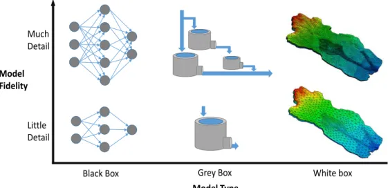
The above section outlined two extremes of model types: mechanistic and data-drivenmodelling. These extremes are referred to as white-box or black-box models, respectively (Breiman, 2001). All mathematical models can conceptually be situa-ted somewhere on the grey scale between or at these two extremes (Refsgaard and Abbott, 1996). Causality and association (specifically correlation) are not mutu-ally exclusive - association at the white end is included into the model by causal relations and at the black end regardless thereof. A grey-box model is a mixture that uses causal relations for the parts of the model that are understood mecha-nistically and adds associative relations to approximate the system behaviour in other model parts. I refer to the black-white scale as model type in Figure 1, as explained in the following.
Just like the grey scale is continuous, the transitions between the model types are smooth. In natural science and engineering, systems and their processes are often represented by conservation laws, as for mass, energy and momentum. Corre-sponding white-box models contain ordinary or partial differential equations (see Equation 2) which fully describe causal relations for all involved variables and parameters. However, it is often not possible to describe every detail of a system by fully resolved physics at all scales, e.g., friction as a meso-scale phenomenon. Then, empirical or data-driven relations have to be employed for which it might be possible to assign physical dimensions as units (even with fractal exponents as in case of friction laws). Yet, they lump properties of the considered system that are not fully resolved or understood, e.g., by friction coefficients. The data-driven paradigm can likewise be used to model the whole system directly as full black-box model (see Equation 3) without the need of any mechanistic description. Illustrative examples of white-box, grey-box and black-box models in hydrosystem modelling with the same objective like stream discharge prediction are shown in Figure 1: finite element models (e.g. von Gunten et al., 2014), conceptual hydro-logic (bucket) models (e.g. Fenicia et al., 2016) or neural network models (Zhang and Zhao, 2012), respectively.
Black Box Grey Box White box Much Detail Model Type Little Detail Model Fidelity
Figure 1: Model conceptuality: model type and fidelity; illustrated by two examples for each model type with different degrees of detail, i.e. a neural network, a bucket-type model and a PDE-based model (from von Gunten et al., 2014) for stream discharge modelling.
In each conceptual modelling type - black, grey or white - there are different levels of fidelity (see Figure 1). Typically, the term fidelity expresses accurate reproduci-bility. In modelling, this can refer to the model output or the model itself in terms of approaching or representing the true system. Here, model fidelity (e.g. Sinsbeck and Tartakovsky, 2015) refers to the number of model elements and the degree of detail or resolution within a particular model type - for which fidelity provides an encompassing and type-independent terminology. In case of black-box neural networks, fidelity refers to the number of nodes within each layer, the number of hidden layers as well as inter- and intra-linking connections, etc. Staying with the example of discharge predictions, high fidelity can mean to have two separate output nodes for base and peak flow. A grey-box model can have different fide-lity stages depending on the amount of sequentially or parallely arranged units or pools (like hydrologic buckets), attached source and sink terms or other functional parts that modify the output like stream discharge. For differential equation-based white-box models like finite element models, the fidelity refers to different levels of spatial or temporal discretization (e.g. Leube et al., 2013), i.e. the grid resolution for solving the underlying equations, coupling of subsurface and surface water flow and further (semi-)physical relationships that refine process descriptions.
Model evaluation and rating usually does not only refer to the model conceptuality, but also to model fidelity. With respect to the scale of the modelling task (spatially, temporally, amount of data, etc.) and the resolution of available model parameters, boundary conditions, input variables and targeted output, the appropriateness of models varies along both categorical axes. Conceptual uncertainty refers to
the degree of appropriateness and, for compactness, is assumed to comprise both categories: model type and model fidelity.
2.1.3 Mathematical Spaces covered by Modelling
Regardless of which model classification system is used, every mathematical model
Mm refers to three different spaces:
• The prediction space Y (a.k.a. data or model output space) contains our quantity of interest (QoI), e.g., hydraulic head or stream discharge. The variables y for model output (predictions) andD for observations (data) of the QoI are situated inY. The dimensions of this space have the units of the QoI. Each observation, i.e., every element inD or new data pointDo, adds
an axis to this space. Models are set up to to match all observations by their output y or yo on the respective axis. Note, that apart from predictions to
meet observed data, prediction might also refer to not (yet) observed states or additional QoI. These can be considered as additional dimensions of Y
yet without measuredDo. Model output is then supposed to yield estimates
for both, measured and unmeasured quantities. However, for quantitative model rating only the dimensions ofY where data is available are considered. Meanwhile, the remaining dimensions provide more information on the mo-del’s plausibility in a qualitative and semi-quantitative manner, e.g., if the magnitude of the estimated but unobserved quantity matches the modeller’s educated guess.
• Theparameter space Ωm encloses the parametersΘmof a certain model, e.g.,
hydraulic conductivity or storage coefficients. Each model Mm has its own
parameter space with parametersΘm. The dimensionality of the parameter
space is defined by the number of model parametersNp,m, which is sometimes
referred to as parametric complexity (Vanpaemel, 2009).
• The model space M is populated by our model(s), e.g., physics-based or bucket-type models. Conceptually, each model Mm can be located
somew-here in this space. However, the dimensions of this model space are not clearly defined. One can think of the dimensions that span this space as: number of model parameters, degree of nonlinearity of functional relations in the model, etc. Nonetheless, there is no comprehensive and complete description of M.
In stochastic modelling, probability distribution are assigned to both, Y and Ω, in order to account for predictive and parametric uncertainty, respectively. Yet, without clear definition of M, the assignment of a probability distribution the model space is not straight-forward without further specification.
2.1.4 Model Space Settings
All members in a model ensemble M (e.g., candidates from Figure 1) can be lo-cated somewhere in M. Therefore, despite being only vaguely defined, we need a conceptual basis for model evaluation and comparison inMunder the finite hypot-heses problem (see Chapter 1; Nearing et al. (2016)), i.e. a qualitative system to formally relate the models in M to the data-generating truth a.k.a. true model
Mtrue. The true model is the exact mathematical description of the system to be modelled, and is often also called the data-generating model or process, respecti-vely (DGM or DGP). The above terms are used synonymously in the following. All observations D are per definition instances of the corresponding distribution of data / predictions from the true model q(y|Mtrue). The way model candidates relate to Mtrue for a certain modelling task at hand can be distinguished by three different M-settings adopted from Bernardo and Smith (1994):
• M-closed: One of the models in the ensemble M is exactly the true model. Yet, it is unknown which one.
• M-complete: None of the ensemble membersMmis the true model. The true
model exists but it has not been possible (yet) to fully formulate it. Although no member fully represents the truth, at least one might still approximate it.
• M-open: None of the ensemble members Mm is the true model; it is
que-stionable whether a tractable true model exists or certain that it does not. Opposed to the other settings, the true model cannot even be conceptually defined due to, e.g., lack of expertise, lack of time, difficulty in conceptuali-zing, or the system is indeed infinitely complex.
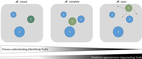
All settings are visualized in Figure 2 as a projection of all model candidates from the M-space onto a 2-dimensional plane (similar to e.g. Sanderson et al., 2015): Between each model’s predictive distributionp(y|Mm) and the DGP’s distribution q(y|Mtrue), distances are evaluated using a statistical distance metric (cf. Section 2.2.4). Then, all models are projected on a 2D plane in a so-called multidimensional scaling process that preserves these mutual distances. Note, that this process has no unique solution regarding the allocation of models on the plane (Sanderson et al., 2015), but this does not limit its suitability for a schematic visualization.
M- closed M- open
Process understanding (Identifying Truth)
Predictive approximation (Approaching Truth)
M- complete 1 2 3 1 2 3 1 2 3 T T T
Figure 2: Illustration of the threeM-settings as 2D projection: M-closed (left), M-complete (center) and M-open (right). The model set comprises three models (blue circles) of different complexity (indicated by the circle size). While in the M-closed and M-complete setting the true model (green circle with “T”) is static in the model space, arrows in the M-open setting depict the true model as “moving target”. The primary objective (process-understanding or predictive approximation) in each setting is visualized by the grey scale (bottom).
In Figure 2, each circle can be considered as the outline of a model’s projection on this plane. The calculated distances between the models can be found between the centers of the circles and the size of each circle sketches the complexity of the model. The transparent green circle resembles the true model and the enumerated opaque blue circles 1, 2 and 3 are model alternatives that are set up to follow
or imitate this truth. Regarding (continuously) taken observations from the true model, Figure 2 can be read as follows:
• In the M-closed setting, one of the models matches the true model exactly which follows from the fact that the DGP can be and is fully conceptualized and also fully formulated. Informative observations allow to identify one model in the set as the true model.
• In the M-complete setting, it can only be incompletely formulated despite full conceptualization. Hence, the true model is not matched by any single model in the ensemble but it is known to be fixed and finite somewhere in
M. Informative observations allow to locate the true model with respect to the models in the set.
• In the M-open setting, the truth cannot even be conceptualized, let alone written down. Then, there is no way to match the truth since the truth itself could not even be located statically on the 2D plane - it “moves” along (yet) unknown or hidden dimensions of M. Informative observations allow to
reveal (previously unknown) features of the true model but without locating it.
These qualitative differences of the M-settings are summarized in Table 1.
Table 1: Qualitative summary of the three M-settings: M-closed, M-complete and M-open with respect to the true model.
Model (pdf)... M-closed M-complete M-open
... can be conceptualized fully fully incompletely
... can be formulated fully incompletely impossibly
... matches actual true model (pdf) fully maybe closely maybe temporarily
When referring to the basic purposes for modelling, i.e., to follow or “process understanding” and to imitate or “predictive approximation”, we can simply vi-sualize these M-settings on a white-to-black scale as in Figure 2: The white end refers to M-closed, while the black end resembles M-open and the grey area in between contains M-complete.
Each end has one dominant objective: At the white end, the goal can be to fully explain the DGP - via identifying the true model from our ensemble of models. At the black end, the objective can only be predictive capability - via selecting one or combining several of the models in the ensemble for obtaining best predictions. This does not mean that the respective other objective is discarded, but every multi-model framework is primarily tailored to accomplish one major objective, depending on what can be achieved in a certain M-setting.
Although pursuing onlyone of the primary objectives, any multi-model framework might thereby still achieve the respective other objective: The correctly identified DGP in theM-closed setting will automatically yield best predictions. Vice versa, the best model (combination) that produces best predictions outside of M-closed might reveal variable associations or functional relations that are the reason for such predictive power. Potentially, these can be translated into a mathematical description that might help to (partially) understand the DGP - even if we know that at the black end, we are not able to fully conceptualize (and write down) the true model. In both cases, the respectively other objective is covered as a side-product while pursuing the major objective.
Coming from the perspective of physical science and engineering, the colors black and white in the extremes directly resemble the respective model categories that we think are able to fulfil the purpose of modelling in the specific M-setting:
physical differential equations) are the closest resemblance of a real-world DGP and therefore fit to the M-closed setting (white end).
• Black-box models are assumed not to contain any physics and are therefore perfectly suited for theM-open setting. There, we expect that the true DGP cannot even be conceptualized and a bottom-up (data-driven) approach for generalization is required at the black end.
The famous “all models are wrong, but some are useful” (Box, 1976) holds outside of theM-closed setting (with increasing severity towardsM-open). Usually, when the word “model” is used, it is implicitly assumed that the modelling task at hand is outside of M-closed - hence the quote is so appealing. However, in a scenario where an allegedly true model of the DGP is formulated and becomes part of the ensemble for process identification, the quote does not hold. A simple example for a true model can be found in the field of electromagnetism. There, the Maxwell-equations provide a true model of electromagnetic phenomena. Hence, under the current state of knowledge about physics, they are considered right and because of this, they are useful as a model.
It is important to internalize what statements can and cannot be made ultimately when comparing models while being in one or the other M-setting: In an actual
M-closed setting, the best model resembles the DGP. There, and only there, it can be called true model. Per definition, the true model is fully consistent with the data, it provides the exact explanation and yields best predictions. Yet, outside of this framework, the model that yields best predictions by no means also resembles the actual DGP - it might not even be close, e.g., when we have a true physical system and use a data-driven approach to successfully mimic it. Even if a model rating clearly shows one model in the ensemble to be superior to the alternatives in terms of predictive power and we think it resembles the truth quite well, we can never state that we found the true model being outside of the M-closed setting. But it still is the objectively best model for predictive approximation of the truth. The unresolvable issue is that we never know which setting applies to our modelling task at hand. However, to handle multiple models in a multi-model framework, this is also not necessary as long as we understand which M-setting is assumed by the applied method. The distinction between the M-settings helps us in two respects:
• To choose a multi-model framework that at least helps us to achieve our primary modelling goal, i.e., to follow (understand) or imitate (predict).
• To correctly interpret the outcome of multi-model frameworks and properly account for conceptual uncertainty.
2.2
Bayesian Inference and Uncertainty Quantification
2.2.1 Uncertainty, Knowledge and Bayesian PriorsUncertainty in modelling arises from two sources: true randomness and lack of knowledge (e.g. Rinderknecht et al., 2012, and references therein):
• True randomness as it appears in quantum mechanics, for example as radi-oactive decay, is called aleatoric uncertainty.
• Lack of knowledge about the system that shall be modelled, its thorough con-ceptualization, the correct mathematical description and all their cascading consequences are referred to as epistemic uncertainty.
Both kinds of uncertainty can mathematically be handled by probabilities (Rinder-knecht et al., 2012), yet with two different perspectives: Frequentist and Bayesian.
Frequentist: Classically, the entry point to probabilities is the quantification of true randomness by frequencies of occurences in an infinite number of repetitions (e.g. Omlin and Reichert, 1999), e.g., for radioactive radiation as result of nuclear decay. Thereby, it is impossible to predict when a certain atom will decay but between a lot of atoms, it is possible to count how many of them decay after a certain time. This so-called frequentist perspective naturally yields probabilities in the sense of aleatoric uncertainty. Ultimately, this kind of uncertainty remains in any physical system and can be fully described by frequency-based probabilities.
Bayesian: Yet, before aleatoric uncertainty dominates, lack of knowledge is the major source of uncertainty. This can hardly be captured by a frequentistic con-sideration of whether something occurs or not. Instead, it can be described by degree of belief in the available knowledge. This is the Bayesian interpretation of probabilities. This kind of belief shall not be confused with arbitrariness or claims that cannot stand scientific reasoning. Only knowledge that follows the scientific paradigm and cannot be clearly falsified by experts can be transferred into proba-bilities that express degree of belief with respect to epistemic uncertainty.
Under the Bayesian paradigm, probabilities can be assigned before any data is available as so-called prior knowledge. Likewise, the distribution of errors bet-ween observations and model predictions that stem from the measurement process can also be considered as belief (Omlin and Reichert, 1999). As most important property, the Bayesian interpretation of probabilities as beliefs allows their upda-ting when new evidence like observed data is available. Although the Frequentist and Bayesian probability interpretations differ, “resulting knowledge quantificati-ons will be cquantificati-onsistent with the axiomatic foundation of probability theory”
(Rin-derknecht et al., 2012). This means that, ultimately, after theoretically all lack of knowledge has been removed, the remaining epistemic uncertainty equals the irreducible aleatoric uncertainty.
Note that, despite being commonly used, the distinction between aleatoric and epistemic uncertainty is also subject to discussion (Nearing and Gupta, 2018). Further, other approaches of uncertainty quantification are not mutually exclusive with probability theory, e.g., information-theoretic tools allow for a broader ana-lysis of uncertainty (cf. Section 2.2.4) in probabilistic forecasting.
The perspective on probabilities as degree of beliefs requires a closer look at the kinds of knowledge or belief that are transferred into (Bayesian) probability distri-butions, i.e., a distinction between objective, subjective and intersubjective kno-wledge (Gillies, 2012; Rinderknecht et al., 2012; Omlin and Reichert, 1999):
• Objective knowledge refers to facts that can be empirically confirmed and also hold in the absence of human opinion.
• Subjective knowledge, in contrast, is based on impressions of individuals that might but do not have to coincide with objective facts.
• Intersubjective knowledge is what several individuals agree upon.
While subjective knowledge appears and disappears with an individual, intersub-jective knowledge remains as long as individuals join and stay with what was agreed upon. From a scientific perspective, intersubjective knowledge of experts about not-man-made systems is supposed to converge towards objective facts. Often, the Bayesian interpretation of probabilities is criticized for its lack of ob-jectivity or directly blamed to be fully subjective (as discussed in, e.g., Gelman et al., 2008). Typically, there is no objective prior knowledge available - there is even an ongoing scientific debate about what a truly objective prior is supposed to look like (van der Linde, 2012; Gelman et al., 2008). In contrast, fully subjective beliefs usually oppose scientific neutrality. Hence, the kind of knowledge that al-lows to conduct Bayesian inference in compliance with scientific requirements is mostly intersubjective (Reichert et al., 2015). Intersubjectivity entails a natural self-correction away from individual perspectives due to averaging of underlying subjective knowledge and incorporation of available facts that can ideally be ob-jectively confirmed. Hence, Bayesian priors should be assigned and confirmed by expert knowledge (O’Hagan et al., 2006). Despite all criticism, the strength of the Bayesian approach is that it forces the modeller to state all induced knowledge and made assumptions explicitly.
In Bayesian (model) inference, we need to internalize that, first, we primarily deal with epistemic uncertainty, and, second, we need to scrutinize prior beliefs and re-spectively assigned probabilities in light of their kind of knowledge. When testing basic physical laws in perfectly controlled and isolated laboratory experiments, the randomness can be objectively described and even be interpreted from a frequen-tist perspective. In applied fields (e.g., hydrosystem modelling), where we work with a predefined limited subset of models and hardly identifiable parameters, objectivity is per se restricted. At the same time, a model comparison that is ba-sed on only subjective assignments of priors can be considered to be manipulated (Gelman et al., 2004) and is therefore non-trustworthy. For a model comparison to be reliable, we have to make sure that we conduct and interpret it from an intersubjective perspective if objective knowledge is unavailable, honouring that uncertainty in model evaluation and comparison is primarily of epistemic nature.
2.2.2 Bayesian Model Inference
Bayesian statistics provide a coherent framework to conduct uncertainty quanti-fication in terms of uncertain knowledge (about model input, output, parameters and the conceptuality itself) for stochastic models (Gelman et al., 2004). Bayes’ theorem thereby is the tool for updating knowledge with respect to new evidence - formally, by conditioning marginal distributions p(·) in order to obtain condi-tional distributions of the form p(·|·). Practically, this enables us to navigate between and link the probabilistic distributions on the three modelling spaces in-troduced in Section 2.1.3, or, more specifically, their contained variablesy (model output/predictions), D (data), Θ (parameters) and M (models). For any given model Mm, Bayes’ theorem writes as:
p(Θm|D, Mm) =
p(D|Θm, Mm)p(Θm|Mm)
p(D|Mm)
(4) The marginal distribution p(Θm|Mm) represents the prior distribution of
parame-ters, i.e., before observationsDof the QoI are considered in modelMm. As
discus-sed in Section 2.2.1, it is suppodiscus-sed to represent intersubjective or even objective knowledge. IncludingDyields the posterior parameter distributionp(Θm|D, Mm)
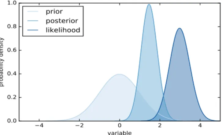
which is the prior distribution conditioned on D. The conditioning is conducted via the likelihood function p(D|Θm, Mm) (cf. Section 2.2.3). Figuratively, the
likelihood “pulls” and “squeezes” the prior while updating it to the posterior as shown in Figure 3.
The denominatorp(D|Mm) in Equation 4 is the marginal likelihood of modelMm,