Competitive coevolutionary algorithm for robust
multi-objective optimization: The worst case
minimization
Ivan Reinaldo Meneghini
Graduate Program in Electrical Engineering Federal University of Minas Gerais Av. Antˆonio Carlos 6627, 31270-901
Belo Horizonte, MG, Brazil
Frederico Gadelha Guimar˜aes
Departament of Electrical Engineering Universidade Federal de Minas GeraisBelo Horizonte, MG, Brazil Email: [email protected]
Antonio Gaspar-Cunha
Institute for Polymers and CompositesUniversity of Minho Campus de Azur´em 4800-058 Guimar˜aes, Portugal
Email: [email protected]
Abstract—Multi-Objective Optimization (MOO) problems might be subject to many modeling or manufacturing uncer-tainties that affect the performance of the solutions obtained by a multi-objective optimizer. The decision maker must perform an extra step of sensitivity analysis in which each solution should be verified for its robustness, but this post optimization procedure makes the optimization process expensive and inefficient. In order to avoid this situation, many researchers are developing Robust MOO, where uncertainties are incorporated in the optimization process, which seeks optimal robust solutions. We introduce a coevolutionary approach for robust MOO, without incorporating robustness measures neither in the objective function nor in the constraints. Two populations compete in the environment, one representing solutions and minimizing the objectives, another representing uncertainties and maximizing the objectives in a worst case scenario. The proposed coevolutionary method is a coevolutionary version of MOEA/D. The results clearly suggest that these competing co-evolving populations are able to identify robust solutions to multi-objective optimization problems.
Index Terms—Robust optimization, coevolutionary Algo-rithms, worst case minimization
I. INTRODUCTION
Engineering optimization problems are often characterized by multiple conflicting objective functions on many variables. The solutions to these problems form the so-called Pareto-optimal set, representing the tradeoff among the objectives. The corresponding image of this set in the objective space, the Pareto front, is characterized by nondominated points, i.e. improving one objective necessarily leads to deteriorating at least one of the other objectives. If the objectives admit a mathematical formulation, approximations of the optimal solu-tions can be achieved by means of multi-objective techniques. Among these, Evolutionary Algorithms (EA) [1, 2] present powerful results in many applications. These stochastic and bioinspired algorithms are able to find good approximations to the Pareto front in terms of convergence, while preserving diversity of the solutions in the estimate.
However, these problems may be affected by different types of uncertainties, such as noise, model inaccuracies, time variation, measurement imprecisions, disturbances and other uncontrolled effects, which might deteriorate the performance
of the designed solutions. The source of these uncertainties can be related to environmental variations (temperature, hu-midity, electromagnetic interference, etc), errors in sensors or measurement equipment, imprecisions in the manufacturing process or implementation of the numerical solution in the real world, simplifications or inaccuracies in the model be-hind the objective and constraint functions, or numerical or model approximations, since the objective functions can be approximated by means of experiments or interpolation (ap-proximation) functions from data [3]. From the practical point of view, optimal solutions that are sensitive to perturbations of the variables or parameters of the model are not desirable. Identifying robust solutions in the estimate of the Pareto set returned by the optimization process is necessary but also can become an additional hindrance for the decision-maker, that should perform a sensitivity analysis of the solutions on the Pareto front in order to assess their robustness to these uncertainties. This analysis could be part of the decision-making process as additional criteria. An alternative to this post optimization procedure is to incorporate the robustness requirement in the optimization process, characterizing the Robust Multi-Objective Optimization (MOO) [4, 5]. The most used techniques in this area incorporate robustness in two different ways:
• Modifying the objective functions, using measures such as averages or deviations;
• Incorporating robustness measures into the problem as additional objectives or constraints.
Since these approaches incorporate the uncertainties of the problem in the objective function or in the constraint functions, it can be applied together with different metaheuristics, such as evolutionary algorithm and simulated annealing. Nevertheless, other interesting ideas and approaches have been presented in the literature, e.g. the use of co-evolutionary algorithms [6], the definition of new relations of dominance based on robustness [7, 8] or the use of interval analysis [9].
In this paper we introduce a coevolutionary approach for Robust MOO, without incorporating robustness measures
nei-ther in the objective function nor in the constrains. Coevo-lutionary algorithms are a class of evoCoevo-lutionary algorithms inspired by the simultaneous evolution of two or more interact-ing populations. Recently, various engineerinteract-ing problems have been solved with this approach [10, 11, 12, 13, 14]. Coello et al. [2] sets coevolution as a reciprocal evolutionary change between species that interact with each other. Coevolutionary algorithms can be categorized into competitive or cooperative algorithms, depending on the nature of the interaction between individuals. In a competition relationship, both species have a negative effect on each other since they are competing for the same resources. In the competitive approach, individuals in the populations compete among themselves, characterizing an arms race or the classicalpredator-preycoevolution. Cooper-ative coevolution is characterized by a beneficial interaction between individuals from each population. Typically, cooper-ative coevolution is used in decomposition of problems into subproblems, and each population evolves partial solutions to each subproblem [13]. The cooperation is required to compute the true fitness of a solution.
In the proposed competitive approach, we create two popu-lations that compete in the environment, one representing the design variables and another representing uncertainties. These populations interact in the computation of the fitness values. The population of variables is evolving towards the Pareto front considering the uncertainties of the second population, while the population of uncertainties is evolving towards dete-riorating the estimate of the Pareto front through perturbations to the variables or to parameters of the objective functions. The proposed co-evolutionary method is a co-evolutionary version of MOEA/D [15]. The results presented in the experiments clearly suggest that these competing co-evolving populations are able to identify robust solutions into multi-objective opti-mization problems.
This work is organized as follows. Section II is a review of robust multi-objective concepts, multi-objective evolutionary algorithm and co-evolutionary algorithms. Special attention is given to the MOEA/D algorithm. Section III presents the pro-posed competitive coevolutionary algorithm, a coevolutionary version of MOEA/D developed for worst case minimization. Results and discussion are presented in Section IV.
II. BACKGROUND A. Robust Optimization
An important reference in robust design is the work de-veloped by the Japanese engineer and statistician Genichi Taguchi [16], with influential contributions to industrial statis-tics and process quality engineering. According to Taguchi [16], quality is measured by the deviation that a functional characteristic presents with respect to its expected value. In this way, a process is said to be robust when it is less sensitive to disturbances in its parameters. Zang et al. [17] defined signal factors as the parameters of a process that determine the configurations to be considered in the robust design, noise factors as factors that are hard to control, causing variability in the system, and control factors as those factors that should
be optimized in order to reduce the sensitivity of the system to the noise factors. Considerf(s, z, x) as a response vector for a determined set of values, where s, z and x represent respectively the signal factors, the noise factors and the control factors. The mathematical formulation presented by Zang et al. [17] for the robust design is given by:
ˆ x= arg min x max s∈V Ez |f(s, z, x)−t|2 (1) where t was the desired response and E was the statistical expectancy (inz), hence characterizing the robust design as a min-max problem.
Later, Deb and Gupta [18] classified the robustness of a solution according to the way the optimization problem was formulated. In the case of single objective optimization, i.e. the minimization of a functionf(x)∈Rwithx∈S:
• A robust solution of Type I is obtained through the minimization of the mean value of f(x) in the defined neighborhood Bδ(x). In other words, a robust solution
is characterized by formulating the problem as the mini-mization of a mean effective function
fef f = 1 |Bδ(x)|
Z
y∈Bδ(x)
f(y)dy,
where |Bδ(x)| is the hypervolume of the neighborhood
Bδ(x).
• A robust solution of Type II is obtained when the perturbation is considered by adding constraints to the problem, which is formulated as the minimization of the functionf(x)subject to
||fp(x)−f(x)||
||f(x)|| ≤η,
where the perturbed function fp(x)can be the mean ef-fective functionfef f(x)or the worst case value observed in the neighborhood Bδ(x).
In the same paper, Deb and Gupta [18] extended these defi-nitions to multi-objective problems, also presenting benchmark functions for Robust MOO.
Jin and Branke [3] presented a classification of sources of uncertainties in optimization problems, based on how these affect the optimization process:
• Presence of noise in the evaluation of objective functions; • Sensitivity of the solution (in the objective space) to
per-turbations in the variables (design space). Those solutions that are immune to this are called robust solutions;
• Fitness function approximations, in cases where the func-tion is expensive to evaluate or the analytical expression is not available;
• Time variations of the objective functions, such that the function, and accordingly its minima, change with time. The authors provided an overview of the main techniques utilized in each case, for instance, implicit or explicit means of the functions, modifications in selection and self-adaptation in evolutionary algorithms, and others [3].
Goh et al. [5] investigated problems with the presence of noise and robust optimization problems, classifying the ways how robustness measures are included in the optimization process as: (i) incorporating noise and/or robustness measures in the variables of the problem as in [4, 19]; (ii) considering these factors as additional objectives to be optimized.
In addition to these methodologies, other ideas had been presented in the literature. Li et al. [6] presented a coevo-lutionary algorithm for the robust design of a permanent magnet machine, considering the worst case minimization. The worst case minimization consists in the following optimization problem: min x∈X max u∈U f(x, u) (2) in which f(x, u) is the objective function, x represents the design variables, u represents the uncertainties. However, their coevolutionary approach is limited to single objective optimization.
Soares et al. [9] presented an interval based multi-objective evolutionary algorithm for robust optimization ([I]MOEA), assuming robustness as insensitivity to variable perturbations. The uncertain parameters are represented with intervals, which results in solution objectives also being represented with intervals. The comparison of solutions is done in the worst-case scenario values of objectives, that is, the values at the border of an interval.
B. Multi-objective optimization
A constrained multi-objective optimization problem (MOP) can be defined as [1, 15] Minimize F(x) = (f1(x). . . fM(x)) subject to x∈X ⊂Rn gj(x)≥0, 1≤j≤J hk(x) = 0, 1≤k≤K (3)
where X is the decision or design space, F(X) ⊂ RM
is the objective space, fi(x) are the objective functions,
gj(x), j = 1, . . . , J are the inequality constraints, and
hk(x), k = 1, . . . , K are the equality constraints. The
constraints of the problem define the feasible region in the decision space and the corresponding image in the objective space.
Multi-objective Evolutionary Algorithms (MOEA) [1, 18, 15] have been successful methods to obtain an approximation of the Pareto front of a MOP. These techniques have been applied in many different fields. In MOEA, new solutions are generated at every iteration from the application of se-lection and genetic operators on an existing population. The performance of solutions is assessed with a fitness function or comparison procedures. Usually, an external population preserves the best estimate of the Pareto front found so far and it is updated accordingly [1].
However, MOEA do not guarantee the robustness of the solutions, which is desirable in many practical applications,
given the presence of uncertainties. Robust optimization seeks for feasible and efficient solutions, that would be less sensitive to perturbations to the variables or parameters of the objective functions [20, 21, 22, 23].
C. MOEA/D
An efficient strategy used in some MOEA is decomposi-tion, in which the MOP is divided into scalar optimization subproblems. One important example of algorithm following this strategy is MOEA/D, proposed by Zhang and Li [15]. In MOEA/D, a set of vectors Λ = {λi ∈ F(X); 1 ≤ i ≤ P},
with population sizeP, is generated before the optimization. These vectors will direct the optimization process. Each indi-vidual of the population is associated to a vectorλj, which is
minimized according to one of the methods below:
• Weighted Sum: Considers a convex combination of the
objectives, which should be minimized in the scalar problem defined by:
minimize gws(x|λ) = M X i=1 λifi(x) (4) withλ= (λ1, . . . , λM)andPMj=1λj = 1
• Tchebycheff: Considers the minimization of the scalar
problem defined by minimizegte(x|λ, z?) = max 1≤i≤M{λi|fi(x)−z ? |} (5) with λ = (λ1, . . . , λM) and z? = (z?1, . . . , zM? ), z ? i = minfi(x).
• Boundary Intersection: Considers the minimization of
the scalar problem defined by
minimize gbi(x|λ, z?) =d1+θd2 (6) withd1= ||(F(x)−z?)Tλ|| ||λ|| ,d2=||F(x)−(z ?+d 1λ)|| andθ >0 is a penalty factor.
In each of the strategies above, the MOP is decomposed into the simultaneous minimization of scalar subproblems defined byg, in which the search is restricted to a group of individuals in the neighborhoodB(x)associated with an elementλi∈Λ.
The MOEA/D is summarized in the following steps:
1) Initialization:
a) Create an empty external population EP, which stores the estimates of the Pareto front;
b) Generate initial population X = {x1, . . . , xP}, withP individuals;
c) Generate P weight vectors Λ for the scalar sub-problems;
d) Calculate the Euclidean distance between any two weight vectors and, for each λi, find the T
closest vectors. Create a neighborhood B(i) = {i1, . . . , iT}referring toλi1, . . . λiT, which are the
T closest weight vectors to λi. Associate each
individual to a single weight vector according to the distance in the objective space or randomly.
e) Evaluate X, makingF Vi=F(xi);
f) Initialize the estimated utopian solution z = (z1, . . . zM), with a problem-specific method. Here
we set zi= minfi(xj)withxj ∈X.
2) Evolutionary cycle:In each iteration, for each
individ-ualxi do:
a) Select two indices at randomk, lfromB(i). Gen-erate new offspring xc with the genetic operators.
b) Update z = (z1, . . . zm): if zj > fj(xc) for any
j = 1. . . , mthen dozj =fj(xc).
c) Update the neighboring solutions: for each j ∈
B(i), ifg(xc|λj, z)≤g(xj|λj, z)then setxj =xc
andF Vj=F(x c).
d) UpdateEP.
The reference pointz in 2b is related to the scalar subprob-lems. In minimization problems, this point corresponds to the smallest value in all objectives, that is,z= (z1, . . . , zm)with
zi = minfi(x).
Note that each individual in the population is evolving to minimize one problem. The minimization of each sub-problem can potentially lead to a Pareto-optimal solution. The search process uses information from solutions to those similar sub-problems, those that belong to the neighborhoodB(i) of
xi.
III. COEVOLUTIONARYROBUSTMOEA/D (C-RMOEA/D)
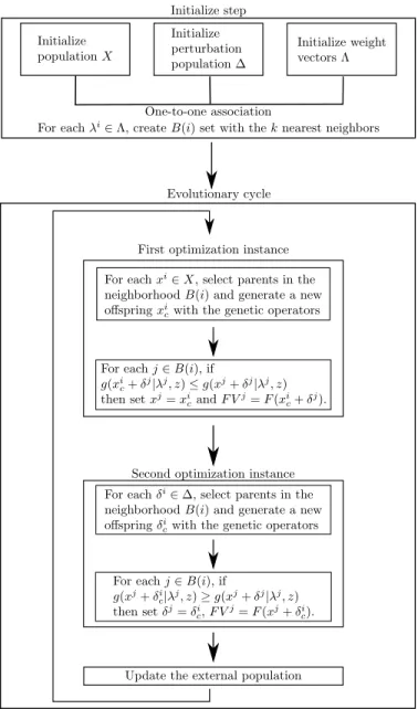
The idea behind the proposed method, called Coevolution-ary Robust MOEA/D (C-RMOEA/D), is the employment of a coevolutionary approach for the solution of robust MOP considering the worst case minimization. The method is based on the basic MOEA/D but under a coevolutionary scheme. The choice for MOEA/D is explained by its characteristic decomposition of the multi-objective problem into scalar sub-problems. The decomposition facilitates the implementation of a coevolutionary approach as it will be shown below.
At each iteration of the evolutionary cycle, two instances of optimization problems are concurrently approached. The population of individuals representing the candidate solutions,
X = {x1, . . . , xP}, is evolving towards the minimization of the function g given the values of perturbations in the population∆. On the other hand, the population∆is evolving towards the maximization of the function g given the values inX. These two processes are in conflict or competition with one another. In other words, the population X, related to the design variables, and the perturbation population∆compete in the environment defined by the robust MOP, see the flowchart in Fig. 1 for details.
Therefore, C-RMOEA/D works with two populations, X, representing the candidate solutions for the design variables, and∆, representing perturbations added to the design variables and/or perturbations in parameters of the functions, both with size P. For each xi = (xi
1, . . . , xin) ∈ X there is a
corresponding δi= (δi
1, . . . , δqi)∈∆ withδji ∈[−, ].
After the initialization steps of C-RMOEA/D, the evolu-tionary cycle begins for both populations. For each xi ∈ X,
Fig. 1. The two instances of the worst case robust optimization: at each itera-tion, the design variables and the uncertainty perturbations are evolved causing the minimization of the functiongin one direction and the maximization in the opposite direction. These two processes are in conflict or competition with one another. In other words, the populationX, related to the design variables, and the perturbation population∆compete in the environment defined by the robust MOP.
two neighboring individuals xia and xib are selected in the
neighborhoodB(i). After that, an offspring is created with the application of the genetic operators (crossover and mutation), producing a new solution xi
c. In this case, we are trying to
minimize the subproblem given by: min
x g(x|δ
i, λi, z) (7)
Notice that in (7), we use the perturbation vectorδi.
There-fore, we should update the neighboring solutions as follows: for eachj∈B(i), if
then setxj=xic andF Vj =F(xic, δj).
Analogously, for each δi∈∆, two neighboring individuals
δi
a andδbi are selected in the neighborhoodB(i). An offspring
δi
c is produced, which is related to the maximization of theg
function:
max
δ g(δ|x
i, λi, z) (8)
In (8), we use the variable xi in order to evaluate δ.
Similarly, we update the neighboring vectors as follows: for each j∈B(i), if
g(δic|xj, λj, z)≥g(δj|xj, λj, z) then setδj =δci andF Vj =F(xj, δci).
Notice that one population is minimizingggiven the values of the perturbations, while the other population is maximizing
g given the values of the variables. These two competing process happen for each pair of xi ∈X andδi∈∆ and for
eachλi∈Λ. The decomposition approach in MOEA/D makes
the coevolutionary approach simpler, since we evolve the perturbations and the variables considering each subproblem independently. A B C z 1 2
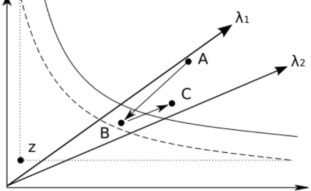
Fig. 2. Illustration of the competitive coevolution in C-RMOEA/D.
Fig. 2 illustrates the competitive coevolutionary process in the objective space. After an offspringxi
cis created, point A is
updated to point B, which decreases the value ofggivenλ1, z. After that, in the evolutionary cycle of∆, it might happen that the point B is updated to point C, which increases the value of
ggivenλ1, z. This alternating process lead to a robust estimate of the Pareto front, considering the worst case analysis. The estimated front contains those solutions that minimize the objectives in the worst case of the perturbations. In one evolutionary cycle, the individuals inXare adjusted according to (7). The estimated Pareto front moves towards the utopian solution in the direction of the front shown in green line. In the evolution of∆, the perturbations are adjusted according to (8). The estimated Pareto front moves away from the utopian solution, in the direction of the front shown in blue line, because the new perturbations found increase the objective function values. By repeating this process, until convergence criteria are met, we can find an estimate of the robust Pareto front, i.e., an estimate that is good even considering the worst case scenario of perturbations for each specific point.
Given that C-RMOEA/D is just an extension of MOEA/D, its implementation is very simple, as presented below.
1) Initialization:
a) Create an empty external population EP, which stores the estimates of the Pareto front;
b) Generate initial population X = {x1, . . . , xP}, withP individuals;
c) Generate population ∆ = {δ1, . . . , δP}, with P
individuals;
d) Associate each individual inX to an individual in ∆.
e) Generate P weight vectors Λ for the scalar sub-problems;
f) Calculate the Euclidean distance between any two weight vectors and, for each λi, find the T
closest vectors. Create a neighborhood B(i) = {i1, . . . , iT}referring toλi1, . . . λiT, which are the
T closest weight vectors to λi. Associate each
individual to a single weight vector according to the distance in the objective space or randomly. g) EvaluateX, makingF Vi =F(xi, δi);
h) Initialize the estimated utopian solution z = (z1, . . . zm), with a problem-specific method. Here
we setzi = minfi(xj, δj)withxj ∈X.
2) Evolutionary cycle:
a) For each individual xi do:
i) Generate an offspring xic with the genetic
op-erators.
ii) Update the neighboring solutions: for eachj ∈
B(i), if
g(xic|δj, λj, z)≤g(xj|δj, λj, z) (9) then setxj=xic andF Vj =F(xic, δj).
b) For eachδi∈∆do:
i) Generate an offspringδci with the genetic oper-ators.
ii) Update the neighboring solutions: for eachj ∈
B(i), if
g(δic|xj, λj, z)≥g(δj|xj, λj, z) (10) then setδj =δci,F Vj=F(xj, δic).
c) UpdateEP.
IV. RESULTS AND DISCUSSION A. Test problems
In order to verify the efficacy of C-RMOEA/D, the bench-mark functions ZDT1 and ZDT2 proposed by Zitzler et al. [24] and TP2, TP2 and TP4 proposed by Gaspar-Cunha et al. [25] were used in this study. In all these functions the perturbation vector is δi = (δi
1, . . . , δqi) ∈ ∆ with δji ∈ [−0.025,0.025].
The choice ofis a parameter defined by the Decision Maker and= 0.025makes the algorithm search for robust solutions in a range of length 2 = 0.05around the optimal solutions by the worst case minimization approach. Considering the
size of the variable range (xi ∈ [0,1] in all problems), the
obtained solutions sets the trade off between the highest value of the goals at an interval of 5% of the range of the variables around the optimal value x?. As the first objective in ZDT1
and ZDT2 functions is f1(x, δ) =x1+δ1, the uncertainty of
x1 is transmitted to this goal, establishing an uncertainty in the objective space.
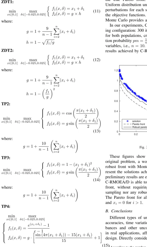
• ZDT1: min x∈[0,1] δ∈[−0max.025,0.025] f1(x, δ) =x1+δ1 f2(x, δ) =g×h (11) where: g= 1 + 9 n−1 n X i=2 (xi+δi) h= 1−pf1/g • ZDT2: min x∈[0,1] max δ∈[−0.025,0.025] f1(x, δ) =x1+δ1 f2(x, δ) =g×h (12) where: g= 1 + 9 n−1 n X i=2 (xi+δi) h= 1− f 1 g 2 • TP2: min x∈[0,1] δ∈[−0max.025,0.025] f1(x, δ) = cos π(x 1+δ1) 2 f2(x, δ) =gsin π(x 1+δ1) 2 (13) where: g= 1 + 10 n−1 n X i=2 (xi+δi) ! • TP3: min x∈[0,1] max δ∈[−0.025,0.025] f1(x, δ) = 1−(x1+δ1)2 f2(x, δ) =gsin π(x 1+δ1) 2 (14) where: g= 1 + 10 n−1 n X i=2 (xi+δi) ! • TP4: min x∈[0,1] max δ∈[−0.025,0.025] f1(x, δ) =e (x1+δ1)−1 e−1 f2(x, δ) =g· sin (4π(x 1+δ1))−15(x1+δ1) 15 + 1 (15) where: g= 1 + 10 n−1 n X i=2 (xi+δi) !
The Pareto front for these benchmark functions is known analytically, thus it is possible to obtain an estimate of the robust front by Monte Carlo simulation over the points on the true Pareto front. This is done by sampling with a Uniform distribution under a Latin Square different values of perturbations for each solution on the front and re-evaluating the objective functions. The worst case corner estimated with Monte Carlo provides an estimate of the robust front.
In our experiments, C-RMOEA/D was run with the follow-ing configuration: 300 iterations, population size ofP= 2101
for both populations, crossover probabilitypc= 1and muta-tion probabilitypm=n1. Each problem was set with 10 design variables, i.e., n= 10. Figures 3, 4, 5, 6 and 7 illustrate the results achieved by C-RMOEA/D.
0 0.2 0.4 0.6 0.8 1 0 0.2 0.4 0.6 0.8 1 1.2 solution Pareto front Robust pareto front
Fig. 3. Test problem ZDT1
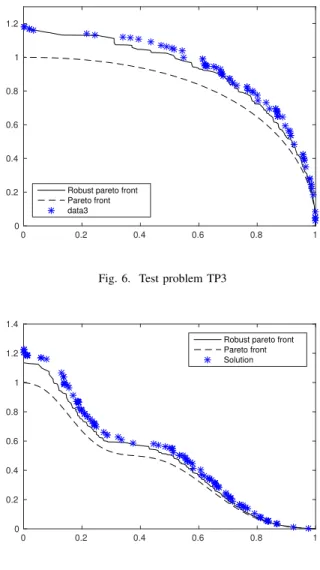
These figures show the non robust Pareto front of the original problem, a worst case estimate applied on the non robust front with Monte Carlo simulation, and the dots rep-resent the solutions achieved by the proposed method. These preliminary results are encouraging evidence that the proposed C-RMOEA/D is able to achieve approximations of the robust front, without requiring additional function evaluations in sampling nor any robust measure of the objective functions. The Pareto front for all problems correspond to x1 ∈ [0,1] andxi= 0 for i >1.
B. Conclusions
Different types of uncertainties, such as noise, model in-accuracies, time variation, measurement imprecisions, distur-bances and other uncontrolled effects, are always present in real applications, affecting the nominal performance of a design. Directly considering them in the optimization process
0 0.2 0.4 0.6 0.8 1 0 0.2 0.4 0.6 0.8 1 1.2
Robust pareto front Pareto front solution
Fig. 4. Test problem ZDT2
0 0.2 0.4 0.6 0.8 1 0 0.2 0.4 0.6 0.8 1 1.2 Pareto front Robust pareto front Solution
Fig. 5. Test problem TP2
lead to the Robust MOO, bringing benefits to the design process. However, usual optimization techniques should be modified and adapted to incorporate robustness requirements into the problem.
This work considered the worst case scenario for the multi-objective optimization problem. A competitive coevolutionary approach based on MOEA/D was introduced for the solution of robust MOP. The algorithm works with two competing populations, one representing the design variables and another representing perturbations added to the design variable or perturbations in parameters of the objective functions. The population of individuals representing the candidate solutions
X is evolving towards the minimization of the functionggiven the values of perturbations in the population ∆. On the other hand, the population ∆is evolving towards the maximization of the functiong given the values inX. These two processes are in conflict or competition with one another.
The results reported in this paper represent preliminary
0 0.2 0.4 0.6 0.8 1 0 0.2 0.4 0.6 0.8 1 1.2
Robust pareto front Pareto front data3
Fig. 6. Test problem TP3
0 0.2 0.4 0.6 0.8 1 0 0.2 0.4 0.6 0.8 1 1.2 1.4
Robust pareto front Pareto front Solution
Fig. 7. Test problem TP4
experiments with the proposed method. These results show the adequacy and efficacy of the method, being able to converge to an estimate of the robust Pareto front. Since two populations are considered in the coevolutionary method, the number of objective function evaluations is doubled in comparison to a single population algorithm. Nonetheless, this additional cost can be small compared to other strategies based on fitness sampling and robust measures. The proposed method is promising in the context of robust multi-objective optimiza-tion, in addition to being an original way of approaching the problem.
Acknowledgements
This work has been supported by the Brazilian agency CAPES. The authors also would like to thank Brazilian agency CNPq (grants 306694/2013-1) and FAPEMIG, for supporting the development of this work.
The first author would like to thank the support given by Instituto Federal Minas Gerais (IFMG), Brazil.
The third author wants to acknowledge the support of FEDER funds through the COMPETE 2020 Programme and
National Funds through FCT - Portuguese Foundation for Sci-ence and Technology under the project UID/CTM/50025/2013.
REFERENCES
[1] K. Deb, Multi-Objective Optimization Using Evolution-ary Algorithms. New York, NY, USA: John Wiley & Sons, Inc., 2001.
[2] C. A. C. Coello, G. B. Lamont, and D. A. V. Veldhuizen, Evolutionary Algorithms for Solving Multi-Objective Problems (Genetic and Evolutionary Computation). Se-caucus, NJ, USA: Springer-Verlag New York, Inc., 2006. [3] Y. Jin and J. Branke, “Evolutionary optimization in uncertain environments – a survey,”Trans. Evol. Comp, vol. 9, no. 3, pp. 303–317, Jun. 2005.
[4] A. Gaspar-Cunha and J. Covas, “Robustness in multi-objective optimization using evolutionary algorithms,” Computational Optimization and Applications, vol. 39, no. 1, pp. 75–96, 2008. [Online]. Available: http://dx.doi.org/10.1007/s10589-007-9053-9
[5] C. K. Goh, K. C. Tan, C. Y. Cheong, and Y. S. Ong, “An investigation on noise-induced features in robust evolutionary multi-objective optimization,” Expert Syst. Appl., vol. 37, no. 8, pp. 5960–5980, Aug. 2010. [6] M. Li, F. G. Guimar˜aes, and D. A. Lowther, “Competitive
co-evolutionary algorithm for constrained robust design,” IET Science, Measurement & Technology, vol. 9, pp. 218–223(5), March 2015.
[7] M. Mlakar, T. Tuˇsar, and B. Filipiˇc, “Comparing solu-tions under uncertainty in multiobjective optimization,” Mathematical Problems in Engineering, vol. 2014, 2014, article ID 817964.
[8] M. Li, R. P. Silva, F. G. Guimar˜aes, and D. Lowther, “A new robust dominance criterion for multiobjective optimization,”IEEE Transactions on Magnetics, vol. 51, no. 3, p. 14, February 2015.
[9] G. L. Soares, F. G. Guimar˜aes, C. A. Maia, J. A. Vas-concelos, and L. Jaulin, “Interval robust multi-objective evolutionary algorithm,” in Proceedings of the Eleventh Conference on Congress on Evolutionary Computation, ser. CEC’09. Piscataway, NJ, USA: IEEE Press, 2009, pp. 1637–1643.
[10] I. Blecic, A. Cecchini, and G. A. Trunfio, “Fast and accurate optimization of a gpu-accelerated {CA} ur-ban model through cooperative coevolutionary particle swarms,”Procedia Computer Science, vol. 29, pp. 1631 – 1643, 2014, 2014 International Conference on Compu-tational Science.
[11] H. Chen, Y. Mori, and I. Matsuba, “Solving the balance problem of massively multiplayer online role-playing games using coevolutionary programming,” Appl. Soft Comput., vol. 18, pp. 1–11, May 2014.
[12] A. Ladjici, A. Tiguercha, and M. Boudour, “Nash equi-librium in a two-settlement electricity market using com-petitive coevolutionary algorithms,” International Jour-nal of Electrical Power & Energy Systems, vol. 57, pp. 148 – 155, 2014.
[13] F. B. de Oliveira, R. Enayatifar, H. J. Sadaei, F. G. Guimar˜aes, and J.-Y. Potvin, “A cooperative coevolu-tionary algorithm for the multi-depot vehicle routing problem,” Expert Syst. Appl., vol. 43, no. C, pp. 117– 130, Jan. 2016.
[14] J. Branke and J. Rosenbusch,Parallel Problem Solving from Nature – PPSN X: 10th International Conference, Dortmund, Germany, September 13-17, 2008. Proceed-ings. Berlin, Heidelberg: Springer Berlin Heidelberg, 2008, ch. New Approaches to Coevolutionary Worst-Case Optimization, pp. 144–153.
[15] Q. Zhang and H. Li, “A multi-objective evolutionary algorithm based on decomposition,” IEEE Transactions on Evolutionary Computation, Accepted, vol. 2007, 2007. [16] G. Taguchi, Introduction to quality engineering: de-signing quality into products and processes. Quality Resources, 1986.
[17] C. Zang, M. I. Friswell, and J. E. Mottershead, “A review of robust optimal design and its application in dynamics,” Comput. Struct., vol. 83, no. 4-5, pp. 315–326, Jan. 2005. [18] K. Deb and H. Gupta, “Introducing robustness in multi-objective optimization,” Evol. Comput., vol. 14, no. 4, pp. 463–494, Dec. 2006. [Online]. Available: http://dx.doi.org/10.1162/evco.2006.14.4.463
[19] J. Ferreira, C. M. Fonseca, J. A. Covas, and A. Gaspar-Cunha, Evolutionary Multi-Objective Robust Optimiza-tion, Advances in Evolutionary Algorithms, X. Zhihui, Ed. InTech, 2008.
[20] A. Ben-Tal, L. E. Ghaoui, and A. Nemirovski, Robust Optimization. Princeton Series in Applied Mathematics, 2009.
[21] D. Pflugfelder, J. J. Wilkens, and U. Oelfke, “Worst case optimization: a method to account for uncertainties in the optimization of intensity modulated proton therapy,” Physics in Medicine and Biology, vol. 53, no. 6, p. 1689, 2008.
[22] W. Liu, X. Zhang, Y. Li, and R. Mohan, “Robust opti-mization of intensity modulated proton therapy,”Medical Physics, vol. 39, no. 2, pp. 1079–1091, February 2012. [23] A. Fredriksson and R. Bokrantz, “A critical evaluation
of worst case optimization methods for robust intensity-modulated proton therapy planning,” Medical Physics, vol. 41, no. 8, 2014.
[24] E. Zitzler, K. Deb, and L. Thiele, “Comparison of mul-tiobjective evolutionary algorithms: Empirical results,” Evolutionary Computation, vol. 8, no. 2, pp. 173–195, 2000.
[25] A. Gaspar-Cunha, J. Ferreira, and G. Recio, “Evolution-ary robustness analysis for multi-objective optimization: benchmark problems,” Structural and Multidisciplinary Optimization, vol. 49, no. 5, pp. 771–793, 2013.