An Execution Model and
High-Level-Synthesis System
for Generating SIMT
Multi-Threaded Hardware
from C Source Code
Ein Ausführungsmodell und High-Level-Synthese System zur Erzeugung von SIMT Multithread-Hardware aus C Quellcode
Zur Erlangung des akademischen Grades Doktor-Ingenieur (Dr.-Ing.) genehmigte Dissertation von Dipl.-Inform. Jens Christoph Huthmann aus Darmstadt
Tag der Einreichung: 03.06.2017, Tag der Prüfung: 21.08.2017 Darmstadt 2017 — D 17
1. Gutachten: Prof. Dr.-Ing. Andreas Koch 2. Gutachten: Prof. Dr.-Ing. Mladen Berekovic
Embedded Systems & Applications Fachbereich Informatik
An Execution Model and High-Level-Synthesis System for Generating SIMT Multi-Threaded Hardware from C Source Code
Ein Ausführungsmodell und High-Level-Synthese System zur Erzeugung von SIMT Multithread-Hardware aus C Quellcode
Genehmigte Dissertation von Dipl.-Inform. Jens Christoph Huthmann aus Darmstadt 1. Gutachten: Prof. Dr.-Ing. Andreas Koch
2. Gutachten: Prof. Dr.-Ing. Mladen Berekovic Tag der Einreichung: 03.06.2017
Tag der Prüfung: 21.08.2017 Darmstadt 2017 — D 17
Bitte zitieren Sie dieses Dokument als: URN:urn:nbn:de:tuda-tuprints-67767
URL:http://tuprints.ulb.tu-darmstadt.de/id/eprint/6776
Dieses Dokument wird bereitgestellt von tuprints, E-Publishing-Service der TU Darmstadt
http://tuprints.ulb.tu-darmstadt.de [email protected]
Die Veröffentlichung steht unter folgender Creative Commons Lizenz:
Namensnennung – Keine kommerzielle Nutzung – Keine Bearbeitung 4.0 Interna-tional
Erklärung zur Dissertation
Hiermit versichere ich, die vorliegende Dissertation ohne Hilfe Dritter
nur mit den angegebenen Quellen und Hilfsmitteln angefertigt zu
haben. Alle Stellen, die aus Quellen entnommen wurden, sind als
solche kenntlich gemacht. Diese Arbeit hat in gleicher oder ähnlicher
Form noch keiner Prüfungsbehörde vorgelegen.
Darmstadt, den
(Jens Christoph Huthmann)
Abstract
The performance improvement of conventional processor has begun to stagnate in recent years. Because of this, researchers are looking for new possibilities to improve the performance of computing systems. Heterogeneous systems turned out to be a powerful possibility. In the context of this thesis, a heterogeneous system consists of a software-programmable processor and a FPGA based con-figurable hardware accelerator. By using an accelerator specifically tailored to a particular application, heterogeneous system can achieve a higher performance that conventional processors.
Due to their increased complexity, it is more complicated to develop applications for heterogeneous systems than for conventional systems based on a software-programmable processor. For programming the software and hardware parts, dif-ferent languages have to be used and additional specialised hardware-knowledge is required. Both factors increase the development cost.
This work presents the compiler framework Nymble which allows to program a heterogeneous system with only a single high-level language. In the high-level language the developer only has to select which parts of the application should be executed in hardware. Nymble then generates a program for the software-processor, the configuration of the hardware, and all interfaces between software and hardware.
All heterogeneous systems supported by Nymble have in common that the soft-ware and hardsoft-ware parts of an application have access to a shared memory. As this memory is external RAM with high access latency, it is necessary to insert a cache between the memory and hardware. With this cache, memory accesses can vary between very short or long access latency depending on whether the data is available in the cache.
To hide long latencies, this thesis presents a novel execution model which allows the simultaneous execution of multiple threads in a single accelerator. Addition-ally, the model enables threads to be dynamically reordered at specific points in the common accelerator pipeline. This capability is used to let other (non-waiting) threads overtake a thread which is waiting for a memory access. Thus, these other threads can execute their calculations independently of the waiting thread to bridge the latency of memory accesses.
Previous works are using execution models which only allow a single thread to be active in the accelerator. In case of a memory access with long latency, the
thread is exchanged with another non-waiting thread. This design of the hardware often causes many resources to lie idle for a significant amount of time.
In contrast, the presented novel execution model dynamically spreads multiple threads over the pipeline. This results in a higher utilisation of the resources by using resources more effectively. Furthermore, the simultaneous execution of multiple threads can achieve similar throughput as multiple copies of a single-threaded accelerator running in parallel.
The new execution model makes it possible to combine the improved through-put of multiple copies with the increased efficiency of simultaneous threads in a single accelerator. Thread reordering allows the new model to be effectively used with a cached shared-memory.
In comparison, between four copies of a single-threaded accelerator and a multi-thread accelerator with four thread (both created by Nymble), a resource efficiency of up to factor 2.6x can be achieved. At the same time, four simulta-neous threads can be up to 4x as fast as four threads executed consecutively on a single accelerator. Compared to other, more optimised compilers, Nymble can still achieve up to 2x faster runtime with 1.5x resource efficiency.
Kurzfassung
Da bei der Leistung von herkömmlichen Prozessoren in den vergangenen Jah-ren eine Stagnation bei der Verbesserung der Leistung zu verzeichnen war, wurde nach neuen Möglichkeiten gesucht die Leistung von Computersystemen zu stei-gern. Heterogene Systeme haben sich als eine leistungsfähige Alternative heraus-gestellt. Im Kontext dieser Arbeit besteht ein heterogenes System in der Regel aus einem mit Software programmierbaren Prozessor und einem konfigurierba-rem Hardwarebeschleuniger. Durch den für jede Anwendung speziell konfigurier-ten Hardwarebeschleuniger können heterogene Systeme eine bessere Leistung als ein herkömmlicher Prozessor erreichen.
Wegen ihrer größeren Komplexität ist es schwieriger für heterogene Systeme Anwendungen zu entwickeln als für ein herkömmliches, rein auf einem Software-Prozessor basiertem System. Da zur Programmierung der Soft- und Hardwarean-teile verschiedene Sprachen verwendet werden müssen und zusätzliche, speziali-sierte Hardware-Kenntnisse erforderlich sind, erhöht dies die Kosten der Entwick-lung.
Diese Arbeit stellt das Compilerframework Nymble vor, welches es ermöglicht, ein heterogenes System allein mit einer Hochsprache zu programmieren. Nach-dem der Entwickler in der Hochsprache festgelegt hat welche Teile in Hardware ausgeführt werden sollen, erzeugt Nymble ein Programm für den Prozessor, die Hardwarekonfiguration und alle Schnittstellen zwischen der Soft- und Hardware. Alle von Nymble unterstützen Systeme haben gemeinsam, dass sich der Software- und Hardwareteil einer Anwendung einen gemeinsamen Speicher tei-len. Da es sich bei dem Speicher um externen RAM mit hoher Zugriffslatenz han-delt, ist es notwendig ein Cachesystem zwischen Speicher und Hardware einzu-fügen. Dies sorgt dafür, dass Speicherzugriffe zwischen sehr kurzer oder langer Latenz variieren können, in Abhängigkeit davon ob die Daten bereits im Cache verfügbar sind.
Um potentielle lange Latenzen zu überbrücken, präsentiert diese Arbeit ein in-novatives Ausführungsmodell, das die simultane Ausführung mehrerer Threads in einem gemeinsamen Hardwarebeschleuniger erlaubt. Zusätzlich ermöglicht das Modell, an bestimmten Punkten in der gemeinsamen Pipeline die Reihenfolge der Threads dynamisch zu ändern. Diese Fähigkeit wird dazu verwendet, dass ein Thread, welcher auf einen Speicherzugriff warten muss, durch andere nicht wartende Threads überholt werden kann. Dadurch können diese unabhängig vom wartenden Threads ihre Berechnungen ausführen und so Latenzen überbrücken.
Bisherige Arbeiten verwendeten ein Ausführungsmodell, in dem jeweils nur ein Thread im Hardwarebeschleuniger aktiv sein konnte und im Falle eines Speicher-zugriffs durch einen anderen Thread ausgetauscht wurde. Durch den Aufbau der Hardware kam es hier oft dazu, dass viele der Ressourcen einen signifikanten An-teil der Laufzeit brach lagen.
Durch seinen innovativen Aufbau verteilt das neue Ausführungsmodell mehrere Threads dynamisch über die Pipeline. Dadurch werden mehr Ressourcen gleich-zeitig sinnvoll genutzt und eine bessere Auslastung erreicht. Weiter erreicht das simultane Ausführen mehrerer Threads einen ähnliche Durchsatz wie mehrere si-multan ausgeführte Kopien eines Hardwarebeschleunigers, welcher jeweils nur einen Thread unterstützt.
Das neue Ausführungsmodell macht es möglich, den erhöhten Durchsatz mit einer verbesserten Effizienz zu kombinieren. Durch das gegenseitige Überholen von Threads ist es möglich das neue Modell effektiv mit einem geteilten Speicher über einen Cache zu verwenden.
Im Vergleich, zwischen vier Kopien eines Beschleunigers für jeweils einen Thread und einem Beschleuniger für vier Threads (beide durch Nymble erzeugt), wird eine Ressourceneffizienz von bis zu Faktor 2,6x erreicht. Dabei sind vier si-multane Threads bis annähernd 4x mal so schnell wie vier auf einem Beschleuni-ger sequentiell ausgeführte Threads. Verglichen mit anderen, besser optimierten Compilern, erreicht Nymble immer noch eine bis zu 2x bessere Laufzeit mit einer 1,5x Ressourceneffizienz.
Danksagung
An dieser Stelle möchte ich mich bei allen Personen bedanken, die mich bei der Anfertigung dieser Arbeit begleitet und unterstützt haben.
Zuerst möchte ich meinen Eltern Gisela und Klaus Huthmann danken, die es mir ermöglicht haben, mich auf meine Arbeit zu konzentrieren.
Auch meine Schwester Alexandra Huthmann gab mir moralische Unterstützung. Meine Familie stand immer hinter mir und dieser Beistand half mir sehr dabei diese Arbeit zu schreiben.
Ein besonderer Dank gilt auch Prof. Dr. Ing. Andreas Koch, der meine Arbeit betreut hat. Neben den Diskussionen und Vorschlägen zu meiner Arbeit, möchte ich mich besonders für das Lektorat meiner Manuskripte bedanken.
Weiterhin möchte ich mich auch bei meinen Kollegen aus der TU Darmstadt bedanken. Die abendlichen Diskussionen mit Benjamin Thielmann haben zur In-spiration meiner Arbeit geführt. Durch die Unterstützung von Julian Oppermann und Björn Liebig konnte ich mich auf die Entwicklung meines Ausführungsmodels konzentrieren. Auch Florian Stock stand immer bereit um Probleme mit der Infra-struktur schnell zu lösen und hatte für viele Fragen eine Antwort. Es war mir ein Vergnügen mit meinen Kollegen zusammenzuarbeiten.
Abschließend möchte ich mich auch bei all meinen Freunden bedanken, welche mich in dieser Zeit begleitet haben.
Contents
Abstract I Kurzfassung III Danksagung V 1 Introduction 1 1.1 Research Contributions . . . 6 1.2 Thesis Structure . . . 8 2 Basics 9 2.1 Program Representations . . . 9 2.1.1 Control-Flow-Graph (CFG) . . . 10 2.1.2 Data-Flow-Graph (DFG) . . . 112.1.3 Static Single Assignment (SSA) . . . 12
2.1.4 Memory-Dependency-Graph (MDG) . . . 12
2.1.5 Control-Data-Flow-Graph (CDFG) . . . 14
2.2 Execution Models . . . 19
2.2.1 Basic Blocks Finite State Machine (FSM) . . . 19
2.2.2 Pipeline . . . 20
2.2.3 Comparison . . . 23
2.2.3.1 Example Favoring BB FSM Model . . . 23
2.2.3.2 Example Favoring Pipeline Model . . . 28
2.2.3.3 Summary of Comparison . . . 31
3 Hardware Execution Model 33 3.1 General Concepts . . . 33
3.1.1 Loop Hierarchy . . . 34
3.1.2 Operation . . . 34
3.1.3 Multi-Cycle Operation (MCO) . . . 35
3.1.4 Variable Latency Operation (VLO) . . . 35
3.1.5 Pipeline Hierarchy . . . 35
3.1.6 HW-SW Communication . . . 36
3.1.6.1 Registers . . . 36
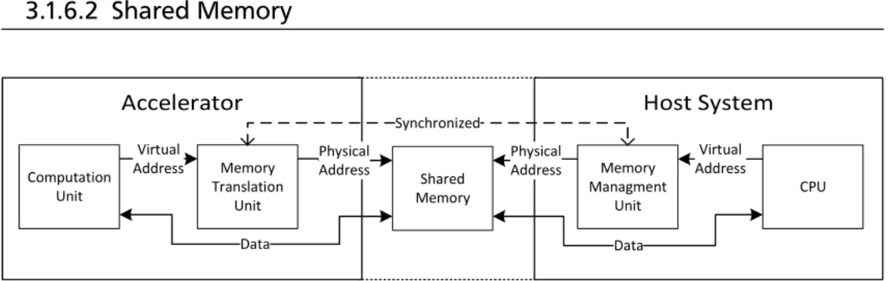
3.1.6.2 Shared Memory . . . 37
3.1.6.3 Hardware-to-Software Calls . . . 37
3.1.6.4 Hardware Invocation Protocol . . . 38
3.2 Pipeline with Static Initiation Interval (II) . . . 39
3.2.1 Example . . . 39
3.2.2 Pipeline level . . . 40
3.2.3 Stage level . . . 42
3.2.4 Operation level . . . 43
3.2.4.1 Multi-Cycle Operation (MCO) . . . 43
3.2.4.2 Variable Latency Operation (VLO) . . . 43
3.2.4.3 Nested Loop . . . 44
3.2.4.4 Memory Access . . . 44
3.2.5 Resource Sharing . . . 44
3.3 Pipeline with dynamic II . . . 45
3.3.1 Example . . . 45
3.3.2 Pipeline level . . . 47
3.3.2.1 Dependency Folding . . . 52
3.3.3 Stage level . . . 53
3.3.4 Operation level . . . 56
3.3.4.1 Multi-Cycle Operation (MCO) . . . 56
3.3.4.2 Variable Latency Operation (VLO) . . . 59
3.3.4.3 Memory Access . . . 59
3.3.5 Resource Sharing . . . 59
3.3.6 Alterations to Hardware Execution Model . . . 62
3.3.6.1 Basic Block Extraction . . . 62
3.3.6.2 Hardware Functions . . . 62 4 Multi-threading 67 4.1 Example . . . 67 4.1.1 Static Interleaving . . . 67 4.1.2 Dynamic Reordering . . . 68 4.2 General Idea . . . 71 4.3 Model Extensions . . . 71
4.3.1 Thread Identifier (TID) . . . 72
4.3.2 Single-/Multi-threaded Stage . . . 72 4.3.3 Pipeline Hierarchy . . . 72 4.3.4 HW-SW Communication . . . 72 4.3.4.1 Registers . . . 73 4.3.4.2 Shared Memory . . . 73 4.3.5 Pipeline level . . . 74 4.3.6 Stage level . . . 82 VIII Contents
4.3.7 Operation level . . . 84
4.3.7.1 Multi-Cycle Operation (MCO) . . . 84
4.3.7.2 Variable Latency Operation (VLO) . . . 85
4.3.7.3 Thread Context Storage (TCS) . . . 87
4.3.8 Queue Usage . . . 88
4.3.9 Placement of Multi-threaded stages . . . 89
5 Basic Block Execution Model 93 5.1 Multi-threading . . . 94
6 High Level Synthesis 97 6.1 Compile Flow . . . 97 6.2 C Input Annotation . . . 98 6.3 Partitioning . . . 98 6.4 CDFG Construction . . . 99 6.4.1 General Construction . . . 100 6.4.2 Condition Construction . . . 101
6.4.3 Memory Dependency Graph Construction . . . 107
6.4.4 CDFG Construction Example . . . 107 6.5 CDFG Optimizations . . . 112 6.5.1 Chaining . . . 112 6.5.2 Constant Propagation . . . 113 6.6 Scheduling . . . 113 6.6.1 ASAP Scheduling . . . 113 6.6.2 Modulo Scheduling . . . 113 7 Target Systems 115 7.1 ACE M5 . . . 115 7.2 DINI . . . 116 7.3 Convey . . . 118 8 Related Work 121 8.1 General . . . 121 8.2 Compiler Frameworks . . . 122 8.2.1 GCC . . . 123 8.2.2 LLVM . . . 125 8.2.3 CoSy . . . 127
8.3 High Level Synthesis Compilers . . . 127
8.3.1 LegUp . . . 127
8.3.2 Bambu . . . 130
8.3.3 DWARV . . . 131
8.3.4 ROCCC . . . 132
8.3.5 CHAT . . . 134
8.4 Summary . . . 136
8.5 OpenMP based Multi-threading . . . 136
9 Evaluation 139 9.1 Measurement . . . 139
9.1.1 Synthesis . . . 144
9.1.2 Simulation . . . 144
9.1.2.1 Removing Memory Impact . . . 145
9.1.3 Local Memory Emulation . . . 146
9.1.4 Runtime Measurement . . . 147
9.2 Efficiency of Multi-Threaded Model . . . 147
9.2.1 Area Efficiency . . . 148
9.2.2 Runtime Efficiency . . . 152
9.3 Optimised usage of optional Multi-Threaded Stages . . . 155
9.3.1 Backwards Removal . . . 156
9.3.2 Profile-Guided Placement . . . 158
9.4 Basic Block Execution Model . . . 161
9.5 Hardware Functions . . . 163
9.6 Clock Frequency . . . 168
9.7 Comparison with other HLS compilers . . . 168
9.8 In-Depth Analysis . . . 176 9.8.1 gsm . . . 176 9.8.2 gemm_blocked . . . 177 9.8.3 gemm_ncubed . . . 180 9.8.4 spmv_ellpack . . . 182 10 Future Work 185 10.1 Mixed Execution Models . . . 185
10.2 Locks, Semaphores and Critical Regions . . . 185
11 Conclusion 187
List of Abbreviations i
Bibliography iii
List of Figures ix
List of Tables xiii
1 Introduction
For the last 40 to 50 years it seemed the improvement of computer performance was bound to increase without ever slowing down. Moore’s Law [Moo06] was an early observation that the number of transistors inside a CPU is doubled every 18 months. This observation motivated many researchers to keep this rate going up until recently.
In the beginning, this rate could be kept by continuously decreasing the size of each transistor. It was noticed by Dennard [Den+74], that a reduction of a transistor’s size by factor of two comes along with a reduction in power consump-tion by a factor of four. However, coming into the 2000s, this could no longer be achieved. The power usage reduction for transistors could not keep up with the reduction of the size. In turn, it becomes increasingly difficult to cool new chips, because more power is concentrated on a smaller area. This led to a stagnation in the increase of clock frequencies for new chips, which provided a major portion of the improvement of CPU performance.
To further increase performance, the goal changed to put multiple computation cores into a single chip to distribute the power across the chip and thus allowing better cooling. With this it was possible to stay within Moore’s Law. However, it became obvious, that in the future, new ways are necessary for even further performance increases. It is assumed that it will not be possible to reach higher performance cost-efficiently by increasing the number of transistors.
Due to this situation, the goal is shifting to use transistors more effectively. This can be achieved by trading programmability for more efficient usage with specialised accelerators. Examples for this are chips for 3D graphics or video ac-celeration.
This reduced programmability limits the application of such fixed accelerators. To combine the advantages of general purpose CPUs and accelerators, so called heterogeneous systems are developed. In these systems computationally intensive parts are offloaded to dedicated accelerators while less intensive calculations stay on the CPU.
Different methods exist to implement such accelerators. The first method is to develop and implement an accelerator for only a single specific application. So called Application-Specific Integrated Circuits (ASICs) implement the accelerator as a fixed custom accelerator hardware in silicon. While providing the best perfor-mance and efficiency, ASICs are the most expensive way to implement a custom accelerator like coprocessors for encryption. Because of their high non-recurring
expenses for development, ASICs are not viable for small quantities. Another, more flexible method is to use Field Programmable Gate Arrays (FPGAs) which can be re-programmed. Though FPGAs have a lower clock frequency and thus provide less performance than ASICs, the re-programmability allows a flexible use for many applications.
One of the biggest challenges in the application development for heterogeneous systems is that a programmer not only has to develop the software but also has to program the hardware. This requires software and hardware development skills, increasing the cost of development and reducing the productivity compared to software only development. The different components of a heterogeneous system make it also more complex to develop for. To reduce the programming difficulty and improve the productivity it would be favourable if the whole system could be programmed using just a software language. To allow this, it is necessary to develop a compiler which automatically translates the software into hardware programming.
These challenges are acknowledged by different academic works (for more de-tails, see Chapter 8). To understand the differences in target architectures a short overview of computing system architectures is presented.
The architecture of computing systems can be broadly grouped into one of the following classes. A typical computer (see Figure 1.1a) consists of a processing unit (the CPU) and an attached memory. As this memory is normally not directly in the CPU both communicate via a bus. As mentioned earlier, today it is common to put multiple cores into a single CPU, which can understood as multiple processing units connected to a single memory shared between the units (see Figure 1.1b).
As the latency of memory could not be decreased by the same degree as the processing speed increased, it became necessary to use memory closer to or even on the processing unit (see Figure 1.1c) or else the memory would bottleneck the whole system [Bac78]. In CPUs this localised memory is typically used as cache for the external main memory. By having the data, which is currently worked on, closer to the processing unit allowed to reduce the latency of the memory accesses and thus improve the system performance. Of course, local memory can also be used together with multiple processing units (see Figure 1.1d).
Finally, there are the cases of having a processing unit without external memory and having such a processing unit connected to one of the other variants over an additional bus (see Figure 1.1e). In that case, the processing unit of the original system is used as a master which has to transfer all data to the slave accelera-tor before it can work on its local data. This leads back to the aforementioned heterogeneous systems.
Many of other academic HLS compiler target the less complex model of an ac-celerator with its own memory and generally assume that all necessary data is already in that memory. With their focus on local memories, many issues of
Processing
Unit Memory
(a)Single processing unit with external memory Processing Unit Memory Processing Unit
(b)Multiple processing units and shared external memory
Memory Processing Unit M em or y
(c)Single processing unit with local and external memory
Processing Unit M em or y Processing Unit M em or y Memory
(d)Multiple processing units with local and shared external mem-ory Memory Processing Unit A (Master) Mem or y Processing Unit B (Slave) Mem or y
(e)Different processing units
Figure 1.1:Overview of computing system architectures
Time
Figure 1.2:Temporal multi-threading by replacing waiting threads
ing shared main memory (through a cache system) do not have to be handled. However, the focus of this work is improving the efficiency of accelerators in a heterogeneous system using shared main memory. Here, both the accelerator and CPU are sharing the same memory (with virtual addresses and pointer).
The fundamental problem is that it is impossible to predict the time required for accessing the shared memory. If the actual time is longer than the predicted, the accelerator has to wait for data. However, when the accelerator is waiting for an access, the resources of the accelerator are unused because there is no data to process. Some works aim to improve this efficiency problem by letting the accelerator work on a different set of data. For more information, see the related work in Chapter 8.
One method to create multiple data sets is to split a problem into tasks which can be computed independently. So if the accelerator waits for data of one task, it can switch to working on another task. This switching of the accelerator between mul-tiple task is called multi-threading or more specifically temporal multi-threading.
Figure 1.2 shows the behaviour over time for two tasks or threads in an acceler-ator. The first thread (red) runs until it reaches the second stage of the accelerator where it has to wait for data (dashed outline). The waiting thread is then ex-changed with another thread (green) which also runs until it has to wait for data at the same stage. However, now the data for the first thread is available and thus the thread is switched back into the accelerator.
Another fundamental problem is that some operators in the accelerator lie idle for a significant portion of the execution time as they are not required in each step. For example, in a pipeline (see Figure 1.3), one step might use four multi-plication operations but all other steps only use a single multimulti-plication. So most of the time, the remaining three operators lie idle (1.3a). By sharing a single real multiplication operator between the four logical operations in the first step, the ef-ficiency can be improved, because this single operator is now always in use (1.3b). However, this comes with the cost that the performance is reduced as the first step takes more time to execute.
Mul
1 Mul2 Mul3 Mul4 Mul 1 Mul 1 Mul 1 Step 1 Step 2 Step 3 Step 4 Mul 1 Step 5 Mul 1 ...
(a)Without operator shar-ing Mul 1 Mul 1 Mul 1 Mul 1 Mul 1 Step 1a Step 1b Step 1c Step 1d Step 2 Mul 1 ... (b)With operator sharing Mul
1 Mul2 Mul3 Mul4 Mul 5 Mul 6 Mul 7 Step 1 Step 2 Step 3 Step 4 Mul 8 Step 5 Mul 9 ... (c)Simultaneous multi-threading
Figure 1.3:Operator sharing example
Extending this sharing to multi-threading means to increase the utilization of operations using multiple simultaneous threads. In the example, multiple threads should be organized in such a way that always one thread is utilizing the four mul-tiplication operations (1.3c). The difference here is that operators are not shared in a single thread but are utilized by multiple threads. Until now, multi-threading in FPGA based accelerators was only used for simple-structured applications.
While this kind of simultaneous multi-threading can improve the performance [LRS83], most prior research (see Chapter 8) focused on creating multiple copies of the accelerator to execute multiple threads in parallel. This was done because there was no method to combine simultaneous and temporal multi-threading in a single accelerator instance with variable latency memory accesses.
With this work I want to show that it is possible to combine these three points: 1. Temporal switching between threads to hide memory latency
2. Simultaneous execution of multiple threads to improve performance 3. Resource sharing between multiple threads to improve efficiency
To achieve this, this work presents a pipeline model with a dynamic distance between iterations. In pipelines, the distance between two iterations is the most important indicator for performance. The smaller the distance, the higher the throughput of the pipeline will be. However, in typical pipeline implementations, the whole pipeline is controlled by a single controller. If the pipeline has to wait at any point, all iterations have to wait, resulting in a reduction of performance. This is increased even further with the integration of simultaneous multi-threading as now multiple threads are waiting.
By using a distributed controller, the presented pipeline model can dynamically change the distance between iterations, which in turn is one of the basics of the proposed simultaneous multi-threading. By integrating modules to store thread context into the pipeline, the enhanced model is able to dynamically reorder threads.
1.1 Research Contributions
This thesis provides the following two main contributions. First, the Nymble HLS compiler framework which is also used in a number of other research projects. Second, a novel multi-threaded execution model where simultaneously executed threads share the resources of a single accelerator instance.
1. Nymble
Nymble is a high-level synthesis framework which can generate FPGA based accelerators for a variety of heterogeneous target systems. The accelerators can be implemented with one of many execution models and in the future the compiler will be able to mix and match multiple models according to the requirements of the application.
While this work uses C as the input language for the high-level synthesis, Nymble was used as a back-end for a domain specific language compiler [Hut+10a; Hut+10c].
In the source code, the programmer can select the hardware part of the appli-cation using simple pragmas. The compiler supports heterogeneous systems with shared memory using virtual addresses and pointers.
Before Nymble was published in [Hut+13; HOK14], it was used in research on load-value prediction [Thi+11; THK11b; THK11a; Thi+12; THK12]. In this research, Nymble was used to create accelerators where the memory accesses can be executed speculatively. When a memory access is executed, a heuristic (load value prediction) returns a speculated value for that access. This allows the pipeline to continue, even when a memory access cannot be finished immediately. When the actual access is finished, the speculated value is compared to the actual value. In case both are equal, a fast-path is used to commit the correct value in later pipeline stages and clear buffers. In case the values differ, these buffers are used to redo the calculation with the corrected value.
Other works based on Nymble were published in [LK16; SOK16].
2. Multi-threaded execution model
The main part of this work is the multi-threaded execution model. The aim of this model is to improve performance and efficiency of pipelined acceler-ators. By allowing other threads to overtake a stalled thread in the pipeline, the throughput is increased. At the same time the resource efficiency is im-proved because all threads share the same accelerator and its operators. Only at some pipeline stages, additional logic is introduced for the reordering of threads. By selectively placing these multi-threaded stages in a insofar single-threaded pipeline, the model achieves a higher efficiency than just using copies of the accelerator for each thread.
The model was published in [HOK14; HK15].
Another contribution is the inclusion of hardware functions. Hardware func-tions are very similar to funcfunc-tions in software, as they can be used from multiple points in the pipeline without implementing them multiple times. This reduces the resource consumption with only a small impact on the execution time for many benchmarks.
Further, this works compares two of the most commonly used execution mod-els for accelerators (basic block and pipelined, see Section 2.2). It will be shown that both have advantages and disadvantages for implementing applications with different characteristics. While the focus of this work lies on the pipelined model, this work shows a method how the presented multi-threading technique can be adapted to the basic block model. It will even demonstrate the possibility of arbi-trarily mixing both models. In the future, this will allow the compiler to select the most suitable model for each part of the application. Table 1.1 shows an overview of all supported execution models and where they are presented and evaluated.
Section
Execution Model Threading Presented Evaluated
Pipeline with Static II Single 3.2 9.1.2.1
Pipeline with Dynamic II Single 3.3 9.1.2.1, 9.7
Pipelined with Dynamic II Multi 4 9.2 - 9.3, 9.5 - 9.8
Basic Block Single 5 9.4
Basic Block Multi 5.1 9.4
Table 1.1:Supported hardware execution models (main model is highlighted)
The presented multi-threading is extensively evaluated to show that it can achieve a 2x improvement in resource efficiency compared to simply duplicat-ing a sduplicat-ingle-threaded pipeline. At the same time, multi-threadduplicat-ing can improve the throughput by a factor of 3.5x compared to consecutively executing four threads. The multi-threaded model is especially efficient for applications with floating point
operations, as the multi-threading overhead is reduced with increased operator complexity.
In comparison to other academic HLS compilers, Nymble achieves comparable results in terms of area and runtime. However, as Nymble focuses on the pipelined model, there are some benchmarks (where a basic block models performs better) for which Nymble is slower. Also, as Nymble targets a scalable shared memory model instead of simpler local memories, Nymble uses more resources for its more complex memory handling and the resulting dynamic iteration intervals in the pipelines.
However, with the inclusion of multi-threading and complex operations (float-ing point) Nymble comes much closer to comparable implementations in terms of resource consumption. For the runtime, it even can execute some benchmarks faster than other sequential implementations.
1.2 Thesis Structure
This work begins with an explanation of compiler basics (Chapter 2). This is followed by explanation and comparison of two general execution models (Sec-tion 2.2). These models describe how the instruc(Sec-tions of an applica(Sec-tion are exe-cuted.
Based on these models, the two different hardware executions models supported by this work (basic block and pipelined) are explained in detail (Chapter 3). Note that at first, these models only allow for single-threaded execution. The multi-threaded enhancement of the main execution model (pipeline) will be explained in the following chapter (Chapter 4).
It is followed by a method to integrate the multi-threading previously shown into the basic block execution model (Chapter 5), which is generally used by the other academic compilers. In the future, the compiler could be extended to select whichever execution model is more suitable for a given part of the application.
After an explanation how the compiler translates an application for a het-erogeneous system to hardware (Chapter 6), the different target systems for heterogeneous execution are shown (Chapter 7). Before the evaluation of the multi-threaded execution model and a comparison with other academic compilers (Chapter 9), an overview of related work is given (Chapter 8). Here, some aca-demic compilers are discussed in detail. Because of references to the presented hardware execution models and multi-threading, the related work was not placed as an earlier chapter.
After the comprehensive evaluation, the work ends with an explanation of future work (Chapter 10) and final conclusion (Chapter 11).
2 Basics
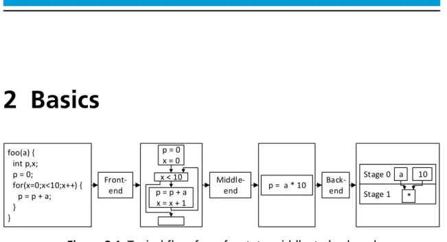
Front-end Middle-end Back-end foo(a) { int p,x; p = 0; for(x=0;x<10;x++) { p = p + a; } } p = 0 x = 0 p = p + a x = x + 1 x < 10 p = a * 10 Stage 1 * Stage 0 a 10Figure 2.1:Typical flow from front- to middle- to back-end
A typical compiler consists of a front-, middle- and back-end (Figure 2.1). The front-end reads and translates the source code into a format easier processable. This format is called the Intermediate Representation (IR). The middle-end is re-sponsible for applying target system independent optimizations on the IR. Finally, the back-end is responsible for applying target system-dependent optimizations and generating the programming of the target system.
The development of a complete set of front-, middle- and back-end is not an easy task. Additionally, all target system-specific steps are only in the back-end. So to focus the development on back-end, it is efficient to use existing front- and middle-ends. gcc [SE16] (Section 8.2.1) and LLVM [LA04] (Section 8.2.2) are the most well known open-source projects providing a set of front- and middle-ends (also including some back-ends).
But the IR of these projects is designed for compilation of applications for gen-eral purpose processors with a gengen-erally sequential execution. For the parallel execution targeting FPGAs, this generic IR has to be translated into a suitable hardware IR.
IRs are used to represent a program’s semantic behaviour. How the application is then actually executed is described through the execution model. For under-standing this process, the basic program representation and execution models are presented in the following sections.
2.1 Program Representations
This section describes the basic program representations used or referenced in this work.
BB1 x = A[i] x != 0 BB3 s = s / 3 BB4 B[i] = s i = i + 1 i < N Start End true false true BB0 s = 0 i = 0 false s = 0;
for(i=0; i<N; i++) { x = A[ i ]; if (x != 0) s = s + 1; else s = s / 3; B[ i ] = s ; } BB2 s = s + 1
Figure 2.2:Conversion of source code to CFG
2.1.1 Control-Flow-Graph (CFG)
A commonly used IR in compilers is the Control-Flow-Graph (CFG) [All70]. CFGs were developed to represent all possible paths of the control flow through each function. A CFG is a directed graph G = (V,E), with nodes V and edges E. Each node contains a list of instructions. Only the last operation in each node can be a (conditional) reference to another node, defining the next node the application executes. Such a node is called a Basic Block (BB). Within a BB, the control always flows from the first to the last instruction in that block. An edge (a,b)
means that the control can flow from node a to node b. Each instruction consists of an operation and its operands. Additionally, the result of the operation can be stored in a variable for later usage.
Figure 2.2 shows the transformation from source code to CFG. The mapping of statements to IR instructions is marked by coloured areas. Edges marked with trueorfalseindicate the control flow in accordance to the result of a conditional instruction at the node’s end. The CFG has total ordering equal to the source code order. It is usually defined by the order given by the programmer through the source code.
2.1.2 Data-Flow-Graph (DFG)
Accompanying the CFG, another representation is often used for a number of opti-mizations and analyses. A Data-Flow-Graph (DFG) [Rod69; Den80] is used to show all paths data can take through the application. It is a directed graph G = (V,E), with nodes V and edges E. Each node represents a single instruc-tion. An edge (a,b) means that the result of instruction a is used in instruction b.
DFGs contain no informations about the control-conditions. Thus, it is not pos-sible to represent the behaviour of multiple assignments to the same variable in BBs on different control-flow paths. In the example, BB2 and BB3 both contain an assignment tos. The following "store to arrayB"-operation has to select one of the previous assignments. It would be theoretically possible to create a DFG for each variant, but the number of DFGs would increase exponentially with the number of such assignments. A partial example for that tentative method is shown in Fig-ure 2.3. To avoid this, the specialised representation form SSA (see Section 2.1.3) was developed. This form ensures that there is only a single static assignment to each variable.
Ignoring this and just creating a DFG results in a DFG as can be seen in Fig-ure 2.4. This DFG has multiple merge-points of data-flows (denoted by zigzag arrows), where the behaviour of which one of the merged data should be used is undefined. + / 0 3 1 Store B[i] (a) + / 0 3 1 Store B[i] (b) + / 0 3 1 Store B[i] (c) + / 0 3 1 Store B[i] (d) Figure 2.3:Tentative DFG variants for variable s and the store
+ / 0 3 1 B[i] + 0 1 < N A[i] != 0 ↯ ↯ ↯
Figure 2.4:Data-Flow-Graph (DFG) for CFG in Figure 2.2
(zigzag arrows denote the merge of two data-flows, which results in undefined behaviour)
2.1.3 Static Single Assignment (SSA)
This form is used to allow easier representation of the data-flow while incorporat-ing the control-conditions.
Each assignment to a variable V creates a new version Vi of the variable. The value is static in the loop iteration that created it. This way, for each use of Vi it can be immediately seen where the value is assigned. Because of this property, the form is called Static Single Assignment (SSA). At nodes with more than one incoming edge, where possible control-flows merge, different versions of the same variable have to be merged into a new version. The pseudo-instruction φ selects the version corresponding to the control-flow actually taken.
SSA is often used with but not limited to CFGs. For example, any source code can also be written in SSA form. The transformation from a normal CFG to SSA was made popular by [Cyt+91].
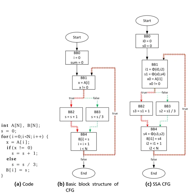
With the additionalφ-instructions, it is now possible to solve the problem with merge of data-flow from multiple sources mentioned in Section 2.1.2. For each merge, the φ-instructions has all sources as its parameters and is integrated into the DFG in the same manner as all other instructions. Figure 2.5 shows the result-ing SSA form for the CFG and DFG in Figure 2.2.
2.1.4 Memory-Dependency-Graph (MDG)
The MDG shows the dependencies between instructions that can access memory. Two memory instructions are dependant on each other when they can access the same memory location. The MDG is a directed graph G = (V,E), with nodes V and edges E are either inter- or intra-iteration dependencies. Thus, E is split into
BB1 s1 = Φ(s0,s4) i1 = Φ(i0,i2) x = A[i] x != 0 BB3 s3 = s1 / 3 BB4 s4 = Φ(s2,s3) B[i1] = s4 i2 = i1 + 1 i2 < N Start End true false true BB0 s0 = 0 i0 = 0 false BB2 s2 = s1 + 1 (a)CFG + / Φ Φ 0 3 1 B[i] + Φ 0 1 < N A[i] != 0 (b)DFG
Figure 2.5:Static Single Assignment (SSA) form of CFG and DFG in Figure 2.2
x = 0 ; while ( x < 5) { tmp = *b ; *a = tmp + 1 ; x = tmp / 2 ; * c = *d + 1 ; } (a)Code inter-iteration intra-iteration
Load (*b) Store (*a) Load (*d) Store (*c)
(b)Memory-Dependency-Graph
Figure 2.6:Memory-Dependency-Graph example
BB0 s = 1 + x t = x – 3 y = s * t (a)CFG + -x 3 1 * (b)DFG
Figure 2.7:Sequential CFG / parallel DFG comparison (ignoring obvious optimizations)
the subsets Eint er and Eint r a. Each node represents an instruction that can access memory. An edge (a,b) means that the instruction a and b can access the same memory location and that a is executed before b in CFG order. The edge is an intra-iteration dependency if a and b are executed in the same loop iteration, otherwise it is an inter-iteration dependency. An edge (a,b), where botha and b are reading accesses, is generally omitted because it does not cause any problems when omitted. Figure 2.6 shows an small code snippet and its MDG.
2.1.5 Control-Data-Flow-Graph (CDFG)
The CFG model is used to represent sequential applications, but it cannot be easily used to represent parallel executed instructions. On the other hand DFGs can easily express instructions that can be executed in parallel. Operations which have no (transitive) connection can be executed in parallel, as they have no data dependencies. Figure 2.7 shows such a case where the parallel execution of the addition and subtraction cannot be easily seen in the CFG (a), while it is obvious in the DFG (b).
But as a DFG has no information about the control-flow or control-conditions, it cannot model the impact of control-flow or control-conditions on the execution. Another form is required, which combines the representation of parallel execution with the control-flow information. An extended DFG is constructed out of a SSA CFG by integrating theφ-instructions into the DFG.
The resulting CDFG is a directed graph G = (V,E) with nodes V represent in-structions and edges E are either data- or control-dependencies. Thus, E is split into the subsets Ed for data-dependencies and Ec for control-dependencies.
The control-flow or control-conditions are integrated into the CDFG in two ways. First, control-dependant data is propagated similar to φ-instructions in the CFG. But as the CDFG contains no CFG like control-flow edges, ψ-instructions are used instead. These ψ-instructions use pairs of data- and control-dependencies (compared to the pairs of data-dependency and control-flow
edge in φ-instructions). If the control-dependency of an input pair is evaluating to true, the corresponding data is propagated. These control-dependencies are constructed in such a way that only one dependency perψ-instruction istrue.
Additionally,φ-instructions only require theimmediate incoming CFG edges for the propagated data selection and rely on the sequential order of the CFG. If the condition of the last branch instructions before the edge is included, it is called an
immediate condition. However, in the CDFG ψ-instructions require the complete conditionunder which data is selected. The complete conditionis a combination of the conditions ofall branch instructions which are evaluated before reaching the BB that contains the instruction.
To clarify this distinction and show why complete conditions are necessary, the examples in Figures 2.8 and 2.10 are used. The first example in Figure 2.8 shows a code segment, its SSA-CFG and the alternatives for evaluating actual values for the control conditions in the CDFG. The CDFG is constructed with only immediate control conditions to show why this is not enough. Note that the CFG in Fig-ure 2.8b and CDFG in FigFig-ures 2.8c to 2.8e omit the normally present edge for the default case of the switch for a cleaner example. When a condition is evaluated totrue, all edges from that condition are coloured in green. When a condition is false, the edges are red. This can be changed by logical operations.
For theψ-instruction at the bottom, marked bya, the selection of the appropri-ate value seems to work correctly for the cases shown in Figures 2.8c and 2.8d. But when examining Figure 2.8e, the ψ-instruction’s control-dependencies both evaluate true at the same time which makes it impossible to select the correct value. The cause for this is that in CFG, the control flow would move from BB0 to BB2 and then to BB3. This does not evaluate the condition y==1 at all, but in the CDFG, such non-executed instructions are generally only handled the correct value selection through ψ-instructions (Instructions with side effects need extra handling, shown shortly). A correctly constructed CDFG with complete conditions
as shown in Figure 2.9 does not have this problem.
The second way of using control-dependencies is to control the execution of in-structions with side-effects such as modification of data through memory accesses. Only if the control-dependency evaluates to true is the instruction executed. In the CFG, the position in the control-flow determines when the operation is exe-cuted. In the CDFG, the control-flow is transformed into a control-dependency which has to evaluatetrueto execute the operation.
In the second example, these control-dependencies for operations with side-effects are shown. In Figure 2.10, three memory access are shown in different branches created by two branch instructions with the conditions A and B. The example contains no φ-instructions. Looking at the CDFG with only immediate conditions (Figure 2.10b), it can be easily seen that again immediate conditions are not sufficient. WhenAandB are used separately, it can happen that either the
s = 0 ; switch( x ) {} case 1 : s = s + 1 ; i f( y==1) break; case 2 : s = s + 2 ; } (a)Code BB0 s0 = 0 switch(x) BB1 s1 = s0 + 1 if (y==1) BB2 s2 = Φ(s1,s0) s3 = s2 + 1 BB3 s4 = Φ(s1,s3) 1 2 false true (b)SSA-CFG + + 1 2 0 y == 1 x == 2 ψ ψ ! x == 1 or a b (c)CDFG alternative 1 + + 1 2 0 y == 1 x == 2 ψ ψ ! x == 1 or a b (d)CDFG alternative 2 + + 1 2 0 y == 1 x == 2 ψ ψ ! x == 1 or a b (e)CDFG alternative 3
Figure 2.8:CDFG with only immediate control conditions
+ + 1 2 0 y == 1 x == 2 ψ ψ ! x == 1 or and and
Figure 2.9:CDFG with complete condition for example in Figure 2.8
store toX orY from BB2 or BB3 is executed together withZ in BB4. The solution again is to use the complete condition as shown in Figure 2.10c.
The algorithm to compute these control-conditions and the construction of the CDFG will be shown in Section 6.4.2.
BB1 Condition A BB2 X[0] = 0 Y[0] = 1BB3 BB0 Condition B BB4 Z[0] = 2 true false true false (a)CFG 0 1 A ! 2 B ! store Z[0] store Y[0] store X[0] (b)CDFG (only imme-diate control con-ditions) 0 1 A ! 2 B ! store Z[0] store Y[0] store X[0] & & (c)CDFG (all control conditions)
Figure 2.10:Multiple memory accesses
2.2 Execution Models
This section will show two general models which describe how an application is executed. Execution models describe the order in which the work is executed. This order can be either decided statically at compile time or dynamically at runtime. Most models use a varying degree of both. However, both basic model shown here use a statically decided order to simplify their explanation.
Both models will start with a simple CPU model as an example for their theoret-ical base model. Then a simplified version of the model is applied to a hardware execution model. These simplified models are then compared. Finally, the hard-ware execution models that are implemented by this work are shown in Chapter 3. The example CPU contains a number of execution phases: Instruction Fetch (IF), Instruction Decode (ID), Execute Instruction (EX), Memory Access (MA) and Register Write Back (WB). Each phase requires one time step or clock cycle to execute its function.
2.2.1 Basic Blocks FSM
For the first model, the CPU can execute only one instruction at time. This means that another instruction can be loaded by the IF unit from memory, only when the previous instruction has been completely executed in all necessary phases. During ID phase it can be decided to skip the execution of EX, MA or WB when it is not needed for a specific instruction. That way the latency of single instruction can vary between 2 and 5 cycles.
The theoretical adaptation of that example into a model is very closely linked to the CFG model. For an application in the form of an CFG, each Basic Block (BB) is seen as a single state in the FSM whose instructions are executed together. While the instructions in the BB can (depending on the implementation) be executed somewhat parallel (example is following shortly), the instructions of only one BB are executed at a time because the FSM has only a single state. Thus, the overall sequential nature CFGs is kept, resulting in simpler control conditions. The execution time in this model is the sum of all BB’s execution time.
Figure 2.11b shows such a FSM, executing the operations of each BB parallel, while sequentially going through the BBs. BB0 calculates the values for s and t and then stores them in a register in-between the basic blocks. The result of the comparator goes to the FSM which controls which BB is executed. Internally, it uses the BBs directly as its state.
When not all operations in a BB can be executed in a single clock cycle, the BB is generally split into multiple BBs so that all operation can be assigned in such a way that the operations in the individual blocks can be executed in a single clock cycle. However, there are also operations that take more than one clock cycle by
BB0 s = 1 + x t = x – 3 a > 0 BB1 y = s * t y = s / tBB1 true false (a)CFG BB1 BB0 + -x 3 1 * s t BB2 / > a 0 FSM Control Data y (b)BB FSM with DFG
Figure 2.11:Executing CFG operations in parallel with a BB FSM (ignoring obvious optimizations)
itself. Here it is not possible to split the BB, as a single operation cannot be split. So instead of splitting the BBs into more BBs, the BBs are subdivided by Execution Basic Blocks (EBBs) (so called for a lack of common distinction to BBs).
Assuming for the example in Figure 2.11 that the division in BB2 takes ten clock cycles, BB2 is divided into ten EBB (see Figure 2.12). Also, both BB1 and BB2 is assigned to a single EBB each. Now, the FSM does not use BBs as states any more, but these EBBs. This assignment of operations to one or more EBB is done by a scheduler during compile time that creates a static schedule.
As each EBB takes exactly one clock cycle, the execution time of a system with this model can be easily calculated by the sum of all executed EBB, which in conse-quence means that it depends on which EBB are executed (more in Section 2.2.3).
This execution model is used by many HLS compilers (see Section 8.3).
2.2.2 Pipeline
For the second model, the CPU can execute multiple instructions simultaneously. This is done by ordering the execution phases into a pipeline with one stage per phase. In this pipeline, the data from one stage can only flow into the next stage. But as soon as the data from an instruction leaves a stage, the stage can work on the data of a new instruction. None of the stages can be skipped, so the time to execute a single instruction is the same for all instructions. Assuming no parallel execution of instructions, the number of cycles to execute multiple instructions
BB1 BB0 + -x 3 1 * s t BB2 / > a 0 FSM y EBB0 Control Data EBB1 EBB2 EBB11
Figure 2.12:BB FSM with EBBs for example in Figure 2.11 (division takes ten clock cycles)
Inst. 1 IF ID EX MA WB Inst. 2 IF ID EX MA WB Inst. 3 IF ID EX MA WB
Cycle 1 2 3 4 5 6 7
Figure 2.13:Pipelined execution of 3 instructions
is the number of instructions minus one, plus the number of cycles for the last instruction. Figure 2.13 shows the execution of three pipelined instructions. For each cycle and instruction the figure shows which stage is used by each instruction. The theoretical adaptation of that example into a model based on the CDFG pro-gram representation is not as straightforward as for the previous representation. Remembering that the CDFG models all control and data dependencies, it is pos-sible to assign (orschedule) each instruction to a specific pipeline stage. These de-pendencies were either inter- or intra-iteration dede-pendencies. While intra-iteration dependencies only affect the schedule of a single iteration, the inter-iteration de-pendencies and their schedules affect when the next iteration can be started. Only if the instructions at the source of the dependency have been executed, the next iteration can be started. The time interval between the re-execution of each in-struction is the so called Initiation Interval (II). As the time is generally measured in clock cycles and each cycle the iterations can move one pipeline stage ahead, the II is also a metric for the distance between two data dependent iterations. It
can be used to determine the effectiveness of the pipeline, smaller II being bet-ter. Assuming that the whole pipeline generally has the same II, the II cannot be smaller than the length of the longest inter-iteration dependency.
A small II is important, because the execution time of the pipelined model de-pends mostly on it. As after II cycles a new iteration can be started, the overall execution time can be calculated by multiplying the number of executed iterations ni t er with the II (assuming that each stage takes one clock cycle). The length of the pipelinelpi peis only really important for the last iteration as only then it is nec-essary to wait until it reaches the end of the pipeline (all other iteration obviously reach the end before the last iteration). However, as the last iteration already moved II stages through the pipeline before it is known that it is really the last iteration, these II number of stages can be removed from the runtime. Thus, the execution time of the pipelined model can be calculated as I I×(ni t er−1) +lpi pe.
Figure 2.14 shows an example of such a pipelined CDFG. It is a very simple loop, adding one to a value read from memory and immediately writing it back to another memory location. The pipeline uses the initoperation (which is true only once) to select the initial zero for the loop counter iin Stage 0. Stage 1 contains multiple operations, the increase of the loop counter by adding one, the loop of array A[i] from memory, and the test for loop termination (the end operation is, however, in the last stage). In Stage 2, the value read from memory is then increased by one and finally written back to array B[i] in Stage 3. The pipeline has an II=2 because the increase ofi requires one clock cycle.
Figure 2.14a shows the behaviour of the pipeline by depicting which stages are active during the pipeline execution. It shows that the execution time calculated with II=2, ni t er =2amd lpi pe=4indeed is2×(2−1) +4=6.
1 2 3 4
Time
Stage
(a)Pipeline behaviour
f o r( i =0; i <2; i++) { B[ i ] = A[ i ] + 1 ; } (b)Code Stage 1 Stage 3 Stage 2 Stage 0 + 1 init ! 0 Load A[i] + Store B[i] 1 >= end 2 (c)Pipelined CDFG
Figure 2.14:Example of a pipelined CDFG (II=2)
2.2.3 Comparison
Both of the previously presented models have their advantages and disadvantages for different applications. This section will discuss the general differences between both models. For that purpose two examples, one that favours each model, will be used for comparison.
The first example (Section 2.2.3.1) will show an application which favours the BB FSM execution model. Also, it will be shown that the favourable model can change depending on the input data. The second example (Section 2.2.3.2) then shows an application which favours the pipeline model.
The discussion will talk about two paths through the loop bodies of the example applications. For each application both paths will be marked by red circles for path PAand a green dashed line for path PB.
2.2.3.1 Example Favoring BB FSM Model
The first example application is defined by a small loop. At the start of each iteration a valuexis loaded from the arrayA. This load uses the loop variableias its offset. Depending on the value of x, the value sis increased by one or divided by 3. In each iteration the valuesis then written to the arrayB, withias its offset. The code of this can be seen in Figure 2.15a.
The CFG, shown in Figure 2.15b, is unbalanced in the loop body. This means that the execution time differs for different paths through the CFG. The path PA (marked by red circles) through the loop body is very short compared to PB (marked by a green dashed line). This is caused by different operations in BB2 on PA and BB3 on PB. While BB2 contains a fast addition (assumed to be executed in one clock cycle), the divider in BB3 is assumed to take ten clock cycles. In fact all operations besides the divider are assumed to take one clock cycle to execute. Note that in a typical system, the array accesses in BB1 and BB4 can take a variable amount of cycles through the cache systems. But for simplicity of the examples, this is omitted here.
As explained in Section 2.2.1, the BB FSM model’s execution time depends on which EBBs are executed, which in this example depends on the input data. In Figure 2.16c, the EBB structure of the application is shown. During the compila-tion the contained operacompila-tions in each BB were transformed into DFGs and then statically scheduled to EBBs. As written as in Section 2.2.1, the execution time for each path corresponds with the number executed EBBs on that path (assuming that each EBB takes one clock cycle). PAexecutes EBBs 1, 2 and 13. PB executes 1, 3 to 12 and 13. Note that both paths have the same EBB in the beginning and end. The difference in the middle is caused by the decision (BB1) between the addition (BB2) or division (BB3). As PAexecutes only three EBBs and PB executes twelve EBBs, the execution time for PA is shorter than for PB. From this follows that, depending on data read fromA[i]in BB1, the execution time of an iteration and, in turn of the entire applications, differs.
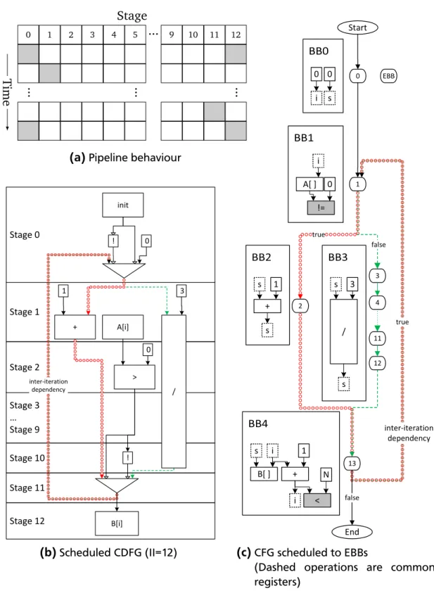
For the pipeline model, the application is transformed into a CDFG which is then scheduled into pipeline stages, as can be seen in Figure 2.16b. Again, in the pipelined model the execution time largely depends on the II. And the II is defined by the longest inter-iteration dependency. In this example, this is the path PB, as shown as in Figure 2.16b. PB has a length of 12 stages (0 to 11), thus taking 12 cycles to execute one iteration. Thus resulting in an II of 12. The store to array b in stage 12 is executed in parallel to stage 0. The behaviour of the pipeline is shown in Figure 2.16a, where active stages are denoted by grey boxes.
As shown as in Section 2.2.2, the execution time of the pipeline model can be as I I×(ni t er−1) +lpi pe. ni t er is the number of executed iterations and the pipeline has a length of lpi pe stages. As after each II number of cycles, a new iteration is started, it thus takes I I ×(ni t er−1) cycles to start the last iteration. This last iteration then has to move through the whole pipeline, requiring lpi pe cycles.
Knowing both execution models, it is now possible to calculate the execution time for them. For the BB FSM, it is necessary to know execution for each possible path, which are PA with an execution time of tA=3 and PB with tB =12. In the pipelined model the execution time depends only on I I = 12and lpi pe =13. For both models the number iterations will be varied in ni t er = [1, 9].
To determine the number of executions (or execution count) EXAand EXB for both paths PA and PB in BB FSM model it is necessary to define the input data for decision in BB1. Because of the very simple decision between zero and non-zero, the input data is defined as the number of zeroes zAcontained in the array A. The overall number of executed iterations corresponds to the size N of arrayA. Thus, the execution time can be calculated with the function tA×(N−zA) +tB ×
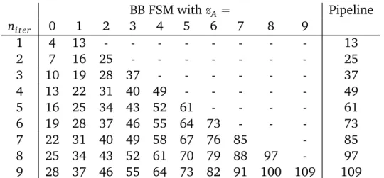
zA. When executing 6 iterations, the time for the Deterministic Finite Automaton (DFA) model is between 15 and 73 cycles for 0 and 6 zeroes in arrayA, respectively. For the pipeline model, the execution time is always 73 cycles. All times can be seen in Table 2.1.
From these numbers it can be seen that the pipeline model generally performs worse than the BB FSM model in case of such an application structure. Only when all iterations in the BB FSM model have to use the longer path PB, the execution time for both models become the same. This means that an application where long operations, which are not executed in each iteration, are influencing the length of the longest inter-iteration dependency and in turn the II, is more suitable for execution with the BB FSM model.
BB FSM withzA= Pipeline ni t er 0 1 2 3 4 5 6 7 8 9 1 4 13 - - - 13 2 7 16 25 - - - 25 3 10 19 28 37 - - - 37 4 13 22 31 40 49 - - - 49 5 16 25 34 43 52 61 - - - - 61 6 19 28 37 46 55 64 73 - - - 73 7 22 31 40 49 58 67 76 85 - 85 8 25 34 43 52 61 70 79 88 97 - 97 9 28 37 46 55 64 73 82 91 100 109 109
Table 2.1:Execution time (#clock cycles) depending on the number of zeros in the input datazAand number of iterationsni t er
i n t A[N] , B[N] ; s = 0 ; f o r( i =0; i<N; i++) { x = A[ i ] ; i f( x != 0) s = s + 1 ; e l s e s = s / 3 ; B[ i ] = s ; } (a)Code BB1 x = A[i] x != 0 BB2 s = s + 1 s = s / 3BB3 BB4 B[i] = s i = i + 1 i < N Start End true false false true BB0 i = 0 sum = 0
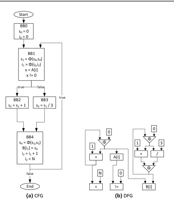
(b)Basic block structure of CFG BB1 i1 = Φ(i0,i2) s1 = Φ(s0,s4) x0 = A[i1] x0 != 0 BB2 s3 = s1 + 1 s2 = s1 / 3BB3 BB4 s4 = Φ(s3,s2) B[i1] = s4 i2 = i1 + 1 i2 < N Start End true false false true BB0 i0 = 0 s0 = 0 (c)SSA CFG
Figure 2.15:Comparison of basic block FSM and pipelined CDFG: advantage FSM (division takes ten clock cycles)
0 1 2 3 4 5 9 10 11 12 T ime Stage ... .. . ... ...
(a)Pipeline behaviour
Stage 12 Stage 11 Stage 10 Stage 3 … Stage 9 Stage 2 Stage 1 Stage 0 A[i] > + ! inter-iteration dependency init ! 0 0 B[i] 3 1 / (b)Scheduled CDFG (II=12) 0 i 0 s A[ ] i != 0 + s 1 s / s 3 s B[ ] i s + 1 i < N true false true Start End false 0 1 3 12 4 11 2 13 inter-iteration dependency EBB (c)CFG scheduled to EBBs
(Dashed operations are common registers)
Figure 2.16:Comparison of basic block FSM and pipelined CDFG: advantage FSM (division takes ten clock cycles)
2.2.3.2 Example Favoring Pipeline Model
The second example application is, like the first, defined by a small loop. Initially, the value of s is initialized to 0, and then modified by each loop iteration. At the start of each iteration, a valuexis loaded from the arrayA. This load uses the loop variable i as its offset. Depending on the value of x, the values is increased or decreased by one. The value ins is then copied tot and divided by 3. Finally,tis written to the arrayB, withias the offset.
Unlike the first application, the CFG (shown in Figure 2.17b) the execution time of the operation in each BB are equal for “parallel” BBs on different paths through the CFG. This means that CFG is balanced, unlike the previous unbalanced exam-ple. The addition in BB2 of path PA(red circles) and the subtraction in BB3 of PB (green dashed line) need the same number of cycles to execute. Both PA and PB then go through BB4 containing the division and write.
Figure 2.18c shows the EBB structure for the DFA model after the transformation into DFGs and scheduling to EBBs. PAuses the EBBs 1, 2 and 4 to 14. PB uses 1, 3 and 4 to 14. Note that both paths have the same number (14) of EBBs and thus have the same execution time. Multiplied by the number of iterations (again N =6) and adding the cycle for EBB0 the execution time of the application in the DFA model is 85.
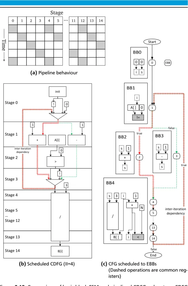
For the pipeline model the application is transformed into a CDFG which is then scheduled into pipeline stages, resulting in the pipeline shown in Figure 2.18b. Unlike the previous example, the longest (and only shown as the loop counteriis omitted) inter-iteration dependency encompasses only a small part of the CDFG.
This allows for the parallel execution of multiple iterations, indicated by an II smaller than the length of the pipeline. This is shown by pipeline behaviour in Figure 2.18a, where active stages are denoted by grey boxes.
The BB FSM model cannot execute multiple BBs at the same time and thus has to execute all iterations sequentially. On the other hand, the pipeline model can initiate the next iteration immediately after the values has been increased or decreased.
Again the execution of the pipeline model can be calculated with I I ×(ni t er− 1) +lpi pe. With I I =4, ni t er =6and lpi pe=15, the execution time of the pipeline model is 35 cycles. Table 2.2 shows a summary of executions times for different number of iterations ni t er.
ni t er 1 2 3 4 5 6 7 8 9
BB FSM 15 29 43 57 71 85 99 113 127
Pipeline 15 19 23 27 31 35 39 43 47
Table 2.2:Runtime (#clock cycles)
s = 0 ; f o r( i =0; i<N; i++) { x = A[ i ] ; i f( x != 0) s = s + 1 ; e l s e s = s − 1 ; t = s / 3 B[ i ] = t ; } (a)Code BB1 x = A[i] x != 0 BB2 s = s + 1 s = s - 1BB3 BB4 t = s / 3 B[i] = t i = i + 1 i < N Start End true false false true BB0 i = 0 sum = 0
(b)Basic block structure of CFG BB1 i1 = Φ(i0,i2) s1 = Φ(s0,s4) x0 = A[i1] x0 != 0 BB2 s3 = s1 + 1 s2 = s1 - 1BB3 BB4 s4 = Φ(s3,s2) t0 = s4 / 3 B[i1] = t0 i2 = i1 + 1 i2 < N Start End true false false true BB0 i0 = 0 s0 = 0 (c)SSA CFG
Figure 2.17:Comparison of basic block FSM and pipelined CDFG: advantage CDFG (division takes ten clock cycles)
0 1 2 3 4 5 11 12 13 14
T
ime
Stage ...
(a)Pipeline behaviour
Stage 14 Stage 13 Stage 5 … Stage 12 Stage 4 Stage 3 Stage 2 Stage 1 Stage 0 A[i] > + -! inter-iteration dependecy init ! 0 0 B[i] 1 1 / 3 (b)Scheduled CDFG (II=4) true false false true 0 Start 1 3 2 4 14 5 13 0 i 0 s A[ ] i != 0 + s 1 s -s 1 s / s 3 B[ ] i + 1 i N < End inter-iteration dependency EBB (c)CFG scheduled to EBBs
(Dashed operations are common reg-isters)
Figure 2.18:Comparison of basic block FSM and pipelined CDFG: advantage CDFG (division takes ten clock cycles)
2.2.3.3 Summary of Comparison
This section showed a comparison of the DFA and pipeline execution model for the use in application-specific hardware. It was shown that for both models appli-cations exist, which execute faster on one of the models. In general, the pipeline model is better for applications which can be scheduled with a small II compared to the overall length. If an application is unbalanced and cannot be scheduled with a small II, the DFA model is better.
While most of the remainder of this work will focus on the pipeline model, later a method to mix both execution models will be shown in Chapter 5 and Sec-tion 10.1. This method will allow to chose the model which is the most appropriate for a given part of the application.
3 Hardware Execution Model
This chapter will describe how the applications are executed on the hardware. All presented execution models are variants of pipelined model (see Section 2.2.2) and use the CDFG representation of the application. In the execution model, the CDFG instructions are executed using hardware operations. In addition to the interaction between the operations (data and control dependencies), it will also be shown how the memory dependencies in the MDG are satisfied during the execution.
The main differences between the presented hardware execution models lie in the handling of the II. While the basic interaction between the instructions is gen-erally the same for all variants, the way iterations are moved through the pipeline is vastly different between them. Nested loops, memory instructions and the han-dling of the MDG is also influenced by the hanhan-dling of the II.
The discussion of the hardware execution models will be done on five different levels; HW-SW communication, Loop Hierarchy, Pipeline, Stage and Operation. The HW-SW communication level will show the interaction between the hardware and software. The Loop Hierarchy level will show how the application’s loop hi-erarchy is handled in the execution model. The HW-SW communication and Loop Hierarchy levels are generally identical for all presented executions models. The pipeline level will show the interactions between the stages in the pipeline. Here it will be shown how the movement of loop iterations between the stages is con-trolled. The general concept of each execution model can be understood by only going as deep as the pipeline level. It also contains most of the differences be-tween the execution models. Because of that, each model description will start with an example on the pipeline level. Then the stage level will show the interac-tions between operainterac-tions. Finally, the operation level will show what is happening in each operation.
Additionally, the pipeline and subsequently each stage is split into data-path and controller. The data-path does all data evaluations (including logical conditions), while the controller decides which and when stages are executed.
3.1 General Concepts
This section will describe concepts common between all hardware execution mod-els.