OPTIMIZATION OF CHANNEL CAPACITY FOR IN-DOOR MIMO SYSTEMS USING GENETIC ALGORITHM
M. A. Mangoud
Department of Electrical and Electronics Engineering University of Bahrain
P. O. Box 32038, Isa Town, Kingdom of Bahrian
Abstract—The geometrical parameters of antenna arrays in a multiple-input multiple-output (MIMO) link that will maximize the ergodic channel capacity of the system are investigated. The problem of selecting the optimum number of the elements at the base station antenna array is also included. The genetic algorithm technique is applied for the optimisation process, using the ergodic capacity as a fitness function. A discrete model based on statistical distribution of the Angle of Arrival (AoA) of the incoming rays is considered. Searching for more compactness in the antenna size and higher system capacity, different array configurations with non-uniform inter-element spacing are considered, such as linear array, circular array and multi-circular array (Star) geometries. Numerical examples that illustrate new designs of non-uniform spaced arrays are presented to show the capability of the developed procedures to optimize the capacity of indoor MIMO systems.
1. INTRODUCTION
the performance of the wireless system under consideration. The channel model employed in this work is a discrete model based on statistical distribution of the AoAs of the incoming rays as in [11] for the receiver part. The spatial correlation matrix at the transmitter will be modeled as in [12–14]. Rician fading channel [15] is also included in the model to consider LOS and NLOS propagations. Previous MIMO antenna design optimization studies are reported in [16] and [17] where the issue of how to appropriately select the number of antennas at the asymmetric base station and mobile units is studied. In [18], for optimizing the MIMO system capacity unequal costs of implementing antennas at both channel ends are considered. However, in this work the cost function is expressed using approximated asymptotic expression for the ergodic capacity calculations. On the other hand, from the geometry selection point of view, Uniform Linear Array (ULA) is the most common geometry in cellular systems. However, Uniform Circular array (UCA) is as an alternative geometry with its enhanced properties. The analysis of fading correlation was carried out for UCA in [12–14]. The results show that the spatial correlation decreases for UCA compared to ULA on average for small and moderate angle spread (AS) for similar aperture sizes. On the other hand, ULA has less spatial correlation than UCA for near broadside angle-of-arrivals with moderate AS. Regarding non-uniform geometries designs, the free standing linear arrays (FSLA) optimized using particle swarm optimization (PSO) was introduced in [19]. Throughout this work, a MIMO channel model based on electric fields including mutual coupling effects is presented. Increased capacity was observed for different 3 dimensional (3D) uniform and non-uniform array configurations compared to conventional 0.5λlength ULA. Another study of outdoor capacity in urban city street grid was performed in [20]. Uniform rectangular array (URA) and uniform cubic array (UCuA) in addition to ULA and UCA with fixed inter-element spacing are considered. The investigations are carried out based on 3D spatial multi-ray realistic physical propagation channel model. It is shown that ULA shows superiority to the other geometries under certain LOS and NLOS propagation conditions and this superiority depends largely on the array azimuthal orientation.
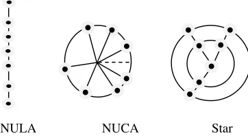
shown in Fig. 1, and these arrays will be optimized at the receive end for uplink indoor MIMO system while we assumed ULA at the transmitter as practical and convenient choice at the mobile unit. The genetic algorithm method (GA) was chosen as the most propitious approach. The optimization will include the selection of the minimum number of radiating elements for the considered arrays.
Also, the placement of the array elements will be optimized for the three array geometries under investigations. The GA search will be subject to propagation environment parameters such as AoAs and AS of the received signal and to antenna array size constraints. The rest of the paper is organized as follows, uplink MIMO channel model is descried in Section 2; Section 3 presents the GA procedures for MIMO antenna array design; Section 4 shows the numerical analysis and discussion; and the paper is concluded in Section 5.
2. SYSTEM MODEL AND SPATIAL CORRELATION CALCULATIONS
The uplink MIMO scenario considered implies that the transmitter is located at the Mobile Unit (MU) and the receiver at the Base Station (BS). The channel was modelled as a multi-clusters scattering environment which means that the signal will arrive at the BS from multiple angles of arrival (AoA), each with angle spread (AS) that is a measure of the angle displacement due to the non-line of sight (NLOS) propagation. DefiningRst(p, q) and Rsr(m, n) as the spatial correlation due to the transmitter and receiver antennas respectively, and assuming that the two links are statistically independent, then the link spatial correlation can be simplified and divided into the transmit and receive parts correlations as follows:
Rs(mp, nq) =Rsr(m, n)×Rst(p, q) (1)
For the ULA at the MU (transmitting side), it is assumed that the mean angle of departure θt is uniformly distributed over [0,2π], as given in [12] as follows:
Rst=Jo
2π(q−p)Dt λ
(2)
be adopted in that case, in order to fit into a convenient thin, flat device. The spatial covariance matrix (Rsr) was computed for different antenna array configurations, since Rsr, a discrete model, was used, based on statistical distribution of the AoAs of the incoming rays. A large number of rays was simulated in order to converge to the IEEE 802.11n channel model (which assumes continuous power angular spectrum (PAS), i.e. angle of arrival of rays). Moreover, antenna arrays consisting of dipole antenna elements were considered, with uniform amplitude excitation and no coupling between array elements. With these assumptions, we can express the spatial correlation matrix for each ray as a product of steering-vectors. Simulating P rays per cluster, the covariance matrix of the cluster is derived as:
Rsr =
n
k=0
a(φo−φp)aH(φo−φp) (3)
wherea(φ) is the steering vector for a generic AoA (φ);φo is the mean AoA of the cluster andφp is the AoA offset with respect to φo for the
pth ray. Note that φp is a random variable with Laplacian probability distribution function. This formula, when substituted in Equation (1), provides the MIMO channel matrix used for the simulations described in the next section. Hereafter the expression of the steering vectors is reported at the AoA φfor different array geometries, as illustrated in Figure 1, according to the following definitions:
• Uniform and Non-uniform spaced Linear Array (ULA & NULA)):
a(φ) =
ejkd1sinφ, . . . , ejkdMsinφT (4)
where are the spacings for the M antennas with respect to the origin of the reference system. We choose the antenna spacings such that the
NULA NUCA Star
total array aperture coincides with the length of the ULA for a fixed number of elements (Mi=1di =M d). If d1 =d2 =. . .=dm =dthen we get the ULA case.
• UCA and NUCA:
a(φ) =
ejkρcos(φ−φ1), . . . , ejkρcos(φ−φM)T (5)
where ρ being the radius of the circular array and φm the angle of themth array element with respect to the reference angle as shown in Figure 1.
• Star and N-star Array:
a(φ) =
1, ejkρcos(φ−φ1), . . . , ejkρcos(φ−φ3),
ejk2ρcos(φ−φ1), . . . , ejk2ρcos(φ−φ3) T
(6)
where star array is designed with (Mr−1)/2 branches and Mr array elements. The correlated Rician Fading MIMO channel Matrix (T) with dimensions (Mt×Mr) at one instance of time can be modelled as a fixed (constant, LOS) matrix and a Rayleigh (variable, NLOS) matrix.
T =
K
1 +KHrıc+
K
1 +KR 1/2
sr HwR1st/2 (7)
whereHw are zero mean and unit variance complex Gaussian random variables that presents the coefficients of the variable NLOS matrix.
Kis the RicianK-factor, andRr andRtare theMr×MrandMt×Mt correlation matrices that include all possible coefficients of spatial correlations between the channel links seen at transmit and receive elements respectively.
3. GA OPTIMIZATION OF ANTENNA CONFIGURATION
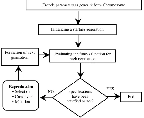
The optimization iterations in GA are called population, which is the unit that the GA optimizer searches in to reach an optimum solution. The optimization iterations in GA are called generations. Pairs of individuals called parents are selected from the population in a probabilistic manner, depending on their fitness function. The objective function defining the optimization goal is called the fitness function, which is a means of assigning a value to each individual in the population. It is a link between the physical problem and the GA optimization process. Children are then generated from the selected pair of parents by applying crossover and mutation processes. Figure 2 shows the design procedure of a GA optimizing technique.
YES NO
Formation of next
generation Evaluating the fitness function for each population
End Initializing a starting generation
Encode parameters as genes & form Chromosome
Reproduction
Selection Crossover Mutation
Specifications have been satisfied or not?
.
.
.
Figure 2. GA optimization procedures.
The optimizing parameters (genes) are the number of array elements at the base station (Mr) and the mobile unit (Mt) and the angles of the elements (φ) that is related to the spacings between them for NUCA/star configurations. Also the radii (ρ) of the receiver circular antenna are included in the numerical results that will be shown in the next section. These variable parameters of the array are placed in the chromosome vector. The fitness function of GA to evaluate the channel capacity in terms of the optimization parameters is:
Fitness =c= log2 det
IM r+ SNR
M t T T
H
(8)
SNR is the average signal to noise ratio; andIM r is the identity matrix with dimensionsMr×Mr. Here we assume equal power transmission across the array elements at the transmitter. Using this procedure, an optimization tool is developed to design arrays with elements whose number, locations and inter-spacing are optimized for higher MIMO channel capacity. The design tool capability will be demonstrated in the following section.
4. NUMERICAL RESULTS
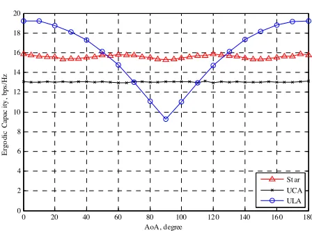
The system performance was analyzed in different propagation conditions: the capacity gain and space diversity advantage attainable with the antenna configurations are shown below. UCA and star configurations and optimization are considered at the BS whereas a ULA is applied at the MU, as shown in Figure 3. Figure 4 shows the ergodic capacity of the UCA and Star and the ULA as a function of Θ (AoA). This example is performed for 7×7 MIMO system with the following assumptions, elements spacingD= 0.5λ for ULA and array radius (ρ) = 0.75λfor UCA and outer Star radius (ρ2) while the inner
Star radius (ρ1) is half ofρ2with elements distributed evenly. AS = 20◦
and SNR = 15 dB is considered. As shown in Figure 4, the UCA and Star outperforms the ULA in particular at endfire (Θ = 90◦) when
Scattering Region
Dominant Reflector (1)
(Mobile unit, MU) ULA Dominant Reflector (2)
Star Base station (BS)
0 20 40 60 80 100 12 0 140 16 0 180 0
2 4 6 8 10 12 14 16 18 20
AoA, degree
E
rgo
di
c Capac
it
y
,
bps
/H
z
St ar UCA ULA
Figure 4. Ergodic capacity versus AoA, one cluster case, 7×7 MIMO ULA, UCA and star system, SNR = 15 dB.
both have the same aperture sizes. However, the ULA performance is better for certain angles-of-arrival near broadside of the ULA Θ = 0◦ and 180◦. Three different examples are presented as follows to show the optimization process results for maximizing MIMO system capacity at different propagation scenarios.
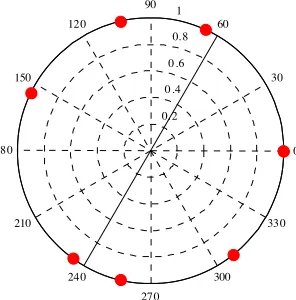
Example 1: The GA was first used to optimize the NUCA geometry and then find the location of elements at nonequal angles. The MIMO system is assumed to be a (7×7) ULA/NUCA with the following assumption: Rician fading channel with K = 10, AS = 20, SNR = 15 and ρ = 0.5λ. Population size is 200 for 20 generations, total ULA length is assumed to be 0.5λ. Here, six angle parameters are used as genes, and each is constrained by±2π/Mr. Figure 5 shows the optimum NUCA geometry. Element locations are at [0, 66, 103, 154, 235, 257, 309] degrees, with system capacity of 11.4 bps/Hz. This shows a little improvement compared to the uniform circular array (UCA) with elements located at equally spaced angles that gives a capacity of 10.01 bps/Hz. However, this run indicates that the GA could be used to design the NUCA geometry effectively, and further investigations are needed for this geometry under different realistic scenarios, especially in cases where more compact arrays are required. Increasing the number of transmit or receive antennas will always increase system capacity. Also, large separations give reduced spatial correlations and higher capacity. Thus, GA optimizing tradeoffs among
0. 2 0 .4
0 .6 0. 8
1
30
210
60
240
90
270 120
300 150
330
180 0
Figure 5. Optimized non uniformly spaced circular array for 7×7 ULA/NUCA MIMO system configuration for AS = 20 and SNR = 15 dB. Elements are at [0 66 103 154 235 257 309], Capacity = 11.4 bps/Hz.
Example 2: we study the optimization of a ULA/UCA system by GA numerical calculation and select the best Mr and Mt numbers for ULA at MU and UCA at BS, also to find the minimum array radius for the UCA to have compact size and space array. We assume SNR = 15 dB and 10 dB, two cases are considered AoA are 0◦ and 90◦. Three constraints are considered here,ρ (UCA radius)<0.5λ,Mt≤9 andMr≤9. The Genes which construct the chromosomes areMb,Mr and ρ. The algorithm has initial number of generations equals 20 and a population size of 200 chromosomes. Table 1 shows the results of the optimum (ULA/UCA) numbers that are (4×9) for all cases and the optimum UCA radius is 0.5λ. It is noted that this case gives higher capacity than the case of (9×9) which is 11.02 bps/Hz and 8.21 for the SNR = 10 and 15 dB respectively.
Table 1. UCA configuration optimization table (ρmax).
SNR AoA As Nt
(ULA)
Nr
(UCA) ρ
Channel capacity
15 0 20 9 4 0.491 12.01
15 90 20 9 4 0.5 12.05
10 0 20 9 4 0.5 8.78
1 2
3
30
210
60
24 0
90
27 0 12 0
300 150
330
180 0
Figure 6. The optimum Star array configuration when As = 5, AOA = 90 case.
0 2 4 6 8 10 12 14 16 18 20 -14
-12 -10 -8
Generation
F
it
ne
ss va
lu
e
Bes t: -12. 4724 Mean: -12. 3346
Best fitne ss Mean fitne ss
Figure 7. The convergence results for the GA run with 20 generations and population size = 200.
The Genes which construct the chromosomes are (Mr, Mt, r1,r2). The algorithm has initial number of generations equals 20 and a population size of 200 chromosomes.
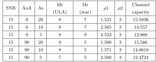
Example 3: a third example is presented to show the GA applications of finding the optimum ULA/Star array configuration (Mr,Mt,ρ1,ρ2) for whichρ1,ρ2 are the inner and outer radii for the star array. We assume SNR = 15 dB; two cases are considered AoA = 0◦ and 90◦; As = 5, 10, 20 cases and the constraint 0.1 < ρ1 <2.9
1 2
3
30
210
60
240
90
270 120
300 150
330
180 0
Figure 8. The optimum Star array configuration when As = 5, AOA = 0 case.
0 2 4 6 8 10 12 14 16 18 20
-14 -12 -10 -8 -6
Ge neration
F
it
n
e
ss va
lu
e
Bes t: -12. 793 Mean: -12 .5296
Best fitness Mean fitness
Figure 9. The convergence results for the GA run with 20 generations and population size = 200.
the convergence results for the GA run. The figures illustrate the best and the mean fitness functions for each generation. While initial set up is 20 generations, converges conditions are included to stop the GA when the mean fitness value becomes equal to the best fitness value over the entire population. For (AoA=0) case study, GA is executed and the output converges in 12 generations as shown in Figure 9.
Table 2. Star configuration optimization table (ρmax).
SNR AoA As Mt
(ULA)
Mr
(star) ρ1 ρ2
Channel capacity
15 0 20 8 7 1.521 3 15.5836
15 0 10 8 7 2.565 3 14.557
15 0 5 8 9 2.523 3 12.868
15 90 20 9 5 1.500 3 15.586
15 90 10 8 5 1.571 3 14.8618
15 90 5 7 5 2.500 3 12.4724
5. CONCLUSION
REFERENCES
1. Jensen, M. A. and J. W. Wallace, “A review of antenna and propagation for MIMO wireless communications,” IEEE Trans. Antenna Propagat., Vol. 52, No. 11, 2810–2824, Nov. 2004. 2. Kermoal, J. P., L. Schumacher, K. I. Pedersen, P. E. Mogensen,
and F. Frederiksen, “A stochastic MIMO radio channel model with experimental validation,” IEEE J. Select., Areas Commun., Vol. 20, No. 6, August 2002.
3. Shiu, D.-S., G. J. Foschini, M. J. Gans, and J. M. Kahn, “Fading correlation and its effect on the capacity of multielement antenna systems,”IEEE Trans. Commun., Vol. 48, No. 3, 502–513, March 2000.
4. Schumacher, L., K. I. Pedersen, and P. E. Mogensen, “From antenna spacings to theoretical capacities — Guidelines for simulating MIMO systems,”IEEE PIMRC 2002, Vol. 2, 587–592, 2002.
5. Teal, P. D., T. D. Abhayapala, and R. A. Kennedy, “Spatial correlation for general distributions of scatterers,”IEEE Sig. Proc. Lett., Vol. 9, No. 10, 305–308, Oct. 2002.
6. Schumachar, L. and B. Raghothaman, “Closed form expressions for correlation coefficient of directive antennas impinged by a multimodal truncated Laplacian PAS,” IEEE Trans. Wireless Commun., Vol. 4, No. 4, 1351–1359, July 2005.
7. Abdi, A., J. A. Bargar, and M. Kaveh, “A parametric model for the distribution of the angle of arrival and associated correlation function and power spectrum at the mobile station,”IEEE Trans. Veh. Technol., Vol. 51, No. 3, 425–434, May 2002.
8. Yong, S. K. and J. S. Thompson, “Three-dimensional spatial fading correlation models for compact MIMO receivers,” IEEE Trans. Wireless Commun., Vol. 4, No. 6, 2856–2869, Nov. 2005. 9. Shafi, M., M. Zhang, A. L. Mousatakas, P. J. Smith, A. F. Molisch,
F. Tufvesson, and S. H. Simon, “Polarized MIMO channels in 3-D Models, measurements and mutual information,”IEEE J. Select. Areas Commun., Vol. 24, No. 3, 514–527, Mar. 2006.
10. Abouda, A. A. and S. G. Hggman, “Effect of mutual coupling on capacity of MIMO wireless channels in high SNR scenario,”
Progress In Electromagnetics Research, PIER 65, 27–40, 2006. 11. Ertel, R. B., P. Carderi, K. W. Sowerby, T. S. Rappaport, and
correlation of MIMO channel,” 58th IEEE Vehicular Technology Conference, VTC 2003, Vol. 1, 94–98, 2003.
13. Tsai, J.-A. and B. D. Woerner, “The fading correlation of a circular antenna array in mobile radio enviroment,”IEEE Global Telecommunications Conference, Vol. 5, 3232–3236, 2001.
14. Xin, L. and Z.-P. Nie, “Spatial fading correlation of circular antenna arrays with laplacian PAS in MIMO channels,” IEEE Antennas and Propagation Society International Symposium, Vol. 4, 3697–3700, 2004.
15. Smith, P. J. and L. M. Grath, “Exact capacity distribution for dual MIMO systems in ricean fading,” IEEE Communications Letters, Vol. 8, No. 1, 18–20, Jan. 2004.
16. Lozano, A. and A. M. Tulino, “Capacity of multipletransmit multiple receive antenna architectures,”IEEE Trans. Inf. Theory, Vol. 48, No. 12, 3117–3127, Dec. 2002.
17. Oyman, O., R. U. Nabar, H. Bolcskei, and A. J. Paulraj, “Tight lower bounds on the ergodic capacity of Rayleigh fading MIMO channels,” Proc. GLOBECOM, 1172–1176, Taipei, Taiwan, R.O.C., Nov. 2002.
18. Du, J. and Y. Li, “Optimization of antenna configuration for MIMO systems,”IEEE Transactions on Communications, Vol. 53, No. 9, 1451–1454, Sept. 2005.
19. Olgun, U., C. A. Tunc, D. Aktas, V. B. Erturk, and A. Altintas, “Optimization of linear wire antenna arrays to increase MIMO capacity using swarm intelligence,” The Second European Conference on Antennas and Propagation, 2007. EuCAP 2007, 1–6, Nov. 11–16, 2007.