https://doi.org/10.17576/jkukm-2019-31(1)-09
Energy Models of Zigbee-Based Wireless Sensor Networks for Smart-Farm
(Model Tenaga untuk Rangkaian Tanpa Wayar Berasaskan Zigbee di Ladang Pintar)Hilal Bello Saida,*, Rosdiadee Nordinb & Nor Fadzilah Abdullahb
aDepartment of Information and Communication Technology, Faculty of Engineering and Environmental Design, Usmanu Danfodiyo University Sokoto, Nigeria.
bCentre of Advanced Electronic & Communication Engineering, Faculty of Engineering and Built Environment, Universiti Kebangsaan Malaysia, Malaysia.
*Corresponding author: [email protected]
Received 20 July 2018, Received in revised form 2 November 2018 Accepted 8 February 2019, Available online 30 April 2019
ABSTRACT
In this paper, we evaluated several network routing energy models for smart farm application with consideration of several factors, such as mobility, traffic size and node size using wireless ZigBee technology. The energy models considered are generic,
MICA and Zigbee compliant MICAz models. Wireless sensor networks deployment under several scenarios are considered in
this paper, taken into account commercial farm specification with varying complex network deployment circumstances to further understand the energy constraint and requirement of the smart farm application. Several performance indicators, such as packet delivery ratio, throughput, jitter and the energy consumption are evaluated and analysed. The simulation result shows that both throughput and packet delivery ratio increases as the nodes density is increased, indicating that, smart farm network with higher nodes density have a superior Quality of Service (QoS) than networks with sparsely deployed nodes. It is also revealed that traffic from the mobile nodes causes increase in the energy consumption, overall network throughput, average end-to-end delay and average jitter, compared to static nodes traffic. Based on the results obtained, the Generic radio energy models consumed the highest total energy, while MICAz energy consumption model offers the least
consumption, having the lowest ‘Idle’ and ‘receive’ modes consumption. The MICAz model also has the lowest total consumed
energy as compared with the other energy models, suggesting that it is the most suitable energy model that should be adopted for future smart farm deployment.
Keywords: Energy models; Smart farm; Internet of Things; WSN; ZigBee; Evaluation INTRODUCTION
The world’s population is expected to reach between 8.3 and 10.9 billion by 2050. The United Nations Food and Agricultural Organizations (FAO) estimate that 70% more
food will need to be produced to feed the additional 2.3 billion people by 2050 (Alexandratos et al. 2012). This develops the increased need for the agricultural sector to devise smarter
and more efficient ways of farming, as farmers seek to
minimize costs and maximize yields.
Smart farming deploys seamless monitoring and controlling system. Achieving high frequency and density monitoring depends on wireless sensor nodes. The smart farm concept is depicted in Figure 1. A smart farm environmental monitoring system based on ZigBee is seen as one of the most practical solutions to these various problems due to its reduced complication and lower cost (Watthanawisuth et al. 2009).
Our major contributions on the subject of smart farming are:
1. Developing a WSN with focus on energy consumption
based on three energy models (Generic, MICA and MICAz)
for potential smart farm application using wireless ZigBee mesh topology. The energy consumption evaluation of the models is presented.
2. Investigating the effect of source traffic, nodes mobility
and nodes size/density in terms of throughput, packets delivery ratio (PDR), average end-to-end delay, average
jitter and energy consumption in the potential smart farm scenarios.
The rest of the paper is structured as follows: Section 2 consists of the related works on smart farm networks evaluation. Section 3 describes the modeling and simulation process of the smart farm environment. In Section 4, experimental results and analysis are presented. Section 5 presents conclusions and suggests possible future works from the paper.
RELATED WORKS
Many studies have presented different smart farm monitoring practices. Other studies investigated the energy consumption in smart farming, while others proposed several methods to minimize smart farm energy consumption.
The work by Jawad et al. (2017) summarized the recent applications, limitations and challenges of WSNs in the
research of agricultural monitoring. Murugan et al. (2017) proposed a method for smart farm monitoring by classifying
it into dense and sparse fields using satellite and drone
information. The studies by Bacco et al. (2018) and N. Zaiedy et al. (2016), observed the monitoring process of different parameters in precision agriculture.
A study by Murya et al. (2017) proposed a method of minimizing the total energy usage of sensor nodes in smart farming using a threshold sensitive hybrid routing technique. In a different study by Jawad et al. (2018), the authors merged the duty cycling energy saving scheme with redundant soil moisture data to formulate a new algorithm called sleep/wake on redundant data (SWORD) for an energy efficient precision
agriculture.
However, the smart farm physical environment is usually instrumented and measured using sensor nodes also known as motes. Several energy models have been developed to depict the real-time performance of these motes for energy
efficiency evaluation. The three energy models considered in
this paper, namely; Generic (Scalable Network Technologies Inc. 2008), MICAz (Crossbow Technology Inc. 2012) and
MICA (Crossbow Technology Inc. 2003) energy models are widely used by researchers and developers in the area of wireless sensor network.
The main feature of the Generic energy model is an estimation of energy consumption for the radios with common
modulation schemes. If not configured, the receiving power
is the same as the idle power consumption. The sleep power value is 0 mW. The MICAz radio energy model is used for
low power wireless sensor network. The data rate of MICAz
is 250 Kbps. The transmission and receiving currents are 19 mA and 17 mA respectively. The MICA Motes radio energy model is pre-configured with the specification of power
consumption of MICA motes. It can transmit approximately
40 kbits per second. In sleep mode, the radio consumes less
than one micro ampere. Receiving and transmission powers are 10 and 25 mA respectively.
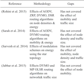
Different researchers have investigated and analyzed the energy consumption of WSNs using these energy models. Table 1 summarized similar works and identified the present
gaps. From Table 1, it can be concluded that there are no previous works that have performed a thorough evaluation on
the effects of energy models, mobility, node size and traffic
size in a future smart farm environment, which is the major contributions of this paper.
FIGURE 1. Conceptual smart farm environment
TABLE 1. Comparison of related literature on energy models for
wireless networking techniques in smart farm Reference Methodology Gaps (Rohini et al. 2015) Effects of AODV, Has not covered
ZRP, DYMO, DSR the effect of routing algorithms mobility and
on node densities & traffic size
energy
(Sarah et al. 2014) Effects of AODV, Has not covered DYMO routing the effect of node
algorithms on density and traffic
mobility & energy size.
(Sarvesh et al. 2014) Effects of modulation Has not covered schemes on energy the effect of using the star mobility, node
topology density and traffic
size.
(Jabbar et al. 2015) Effects DYMO and Has not covered MP OLSR routing the effect of node algorithms on mobility.
network& traffic size SYSTEM MODEL
The idea behind this model was started by the need to build a reliable model of a wireless sensor network for smart farm application using ZigBee technology. A network size of 1500m × 1500m is selected in this study to represent a
commercial farm field area, which represent average farm
size of 234 acres (MacDonald et al. 2013).
The simulation was carried out using Qualnet network
simulator considering five different scenarios. All scenarios
consist of a number of reduced function devices (RFD) as
ZigBee end devices (ZED), full function devices (FFD) as
ZigBee routers (ZR) and one other FFD as PAN coordinator
also called the ZigBee coordinator (ZC). These properties
are set on the MAC layer settings of the Qualnet simulator
software.
The proposed mesh topology network is achieved by
configuring all mobile nodes and outermost static nodes as RFD. All other internal nodes (ZRs and one PAN coordinator)
are set as FFDs. ZC and ZR emit Regular Beacon Frames, which includes control information, such as address identifier and
operation channel. The beacon frames are advertised by all
The number of selected sensor nodes is 20, 30 and 40 so that they are enough to cover the farm perimeter in terms of communication capability, taking into account the ZigBee transmission distance that is limited to maximum of 110 meters (Kuzminykh et al. 2017). Moving devices on the farm,
which are mainly planted on drones, fleet machines such as
tractors, and living stocks such as cows have low mobility, which is set as 3m/s in the simulation.
Meanwhile, examples of static nodes on the farm are plant, soil and environment monitoring sensors, such as soil moisture, pH level and wind direction. Since the network is going to be partially mobile with partly mobile and other static nodes, AODV routing protocol will be considered since it is
the best routing protocol in a partially mobile WSN condition
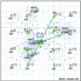
(Sharma et al. 2015). Mesh topology is used because all the radio modules communication is based on broadcast and offer backup and reliability in the event that one of the nodes is fails to operate. The mesh topology architecture used in this study is shown in Figure 2.
In this simulation, the transmission is carried out for 2000 seconds (about 30 minutes), which is selected to allow for substantial battery power depletion and a large amount of packets to be exchanged. However, in real-world implementation, the transmit duration can be set either hourly or at several hours’ interval, thus helps to prolong the battery life. The shorter (lighter colored) arrows emanating from the nodes in the simulation scenario represent the beacon frames.
The first three scenarios are simulated three times each
for Generic, MICAz and MICA radio energy models, while the fourth and fifth scenarios are run once with the MICAz
energy model.
The CBR sending devices are selected carefully in all
scenarios so that the probable number of hops to reach the
PAN coordinator (ZC) is justified for all scenarios. Table 2
summarizes the simulation parameters used.
There are 5 different scenarios considered in the simulation to have better evaluation in terms of nodes density,
mobility and traffic for future smart farm. The scenarios are
summarized in Table 3.
In the first three scenarios, the number of nodes is varied, but with the same number of traffic sources. Four CBR traffic
from 3 static and 1 mobile source is used in Scenarios 1, 2 and 3. Although there is no schedule set for the nodes to send their information, we assumed that more than 1 node can be uploading their data at the same time within the 2000 seconds
window. Therefore, 4 traffic sources are used to receive
enough packets at the sink node within the set parameters to have a clear margin between the different results. For each scenario, Generic, MICAz and MICA radio energy models
are simulated. The energy usage of the WSN consumption
modes such as transmit, receive, sleep and idle are evaluated. Scenario 3 is shown in Figure 3.
The fourth and fifth scenarios are modifications of
the second scenario with the same number of nodes but
different traffic size. The number of active traffic applications FIGURE 2. Proposed mesh network model
The Constant Bit Rate (CBR) traffic source and destination have time synchronization with fixed intervals,
packet size, and stream duration which make it suitable for our smart farm similation. The mobile and static nodes send
CBR traffic (darker arrows extending to the ZC node as shown
in Figure 3 and Figure 4) to the PAN coordinator (ZC) located
in the middle of the smart farm.
FIGURE 3(a). Scenario 3; 40 nodes with CBR from 3 static and 1
mobile node
FIGURE 3(b). Scenario 4; 30 nodes with CBR from 3 static and 5
within the simulation time are doubled here, with 8 nodes sending CBR traffic instead of the 4 nodes in scenario 2. Four mobile and four static traffic sending nodes are respectively
added to the initial four CBR nodes present in the previous
scenarios (scenario 2) so as to have a uniform and double
traffic size in these two scenarios. These two last scenarios
are developed to further expand the smart farm evaluation
scope from nodes density to include the number of traffic
sending applications.
However, due to the assumption that the traffic
application originating from mobile nodes will have a different performance behavior from that of static nodes, we
first designed a smart farm environment in Scenario 4 to have 4 additional mobile traffic sending nodes, making the traffic
to originate from 3 static and 5 mobile nodes as shown in the
setup in Figure 4. The fifth scenario, however, is designed to have its traffic originating from 7 static and 1 mobile node.
The consumed energy of the WSN modes such as transmit,
receive, sleep and idle are evaluated.
RESULTS AND DISCUSSIONS
THROUGHPUT
Throughput is the average rate of successful data packets received at the destination. Figure 5 shows the throughput of Scenarios 1 to 5.
The throughput is seen to be increasing as the number of nodes increases. This is as a result of the increased nodes density in the smart farm. It is also observed based on Scenarios 4 and 5 that the addition of CBR applications
from mobile sources presented an increase in throughput by a higher value. This hike is supported by the study carried out by Grossglauser (2002), where it is demonstrated that
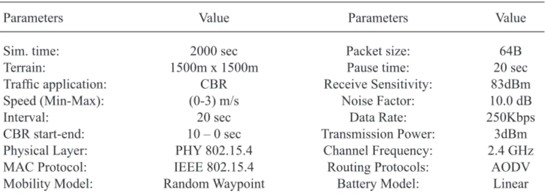
TABLE 2. Simulation parameters
Parameters Value Parameters Value
Sim. time: 2000 sec Packet size: 64B
Terrain: 1500m x 1500m Pause time: 20 sec
Traffic application: CBR Receive Sensitivity: 83dBm
Speed (Min-Max): (0-3) m/s Noise Factor: 10.0 dB
Interval: 20 sec Data Rate: 250Kbps
CBR start-end: 10 – 0 sec Transmission Power: 3dBm
Physical Layer: PHY 802.15.4 Channel Frequency: 2.4 GHz
MAC Protocol: IEEE 802.15.4 Routing Protocols: AODV
Mobility Model: Random Waypoint Battery Model: Linear
TABLE 3. Summary of simulation scenarios
Scenario No. of nodes No. & type of traffic Traffic Source Energy Model
1 20 nodes 4 CBR 3 static and 1 mobile Generic, MICAz, MICA
2 30 nodes 4 CBR 3 static and 1 mobile Generic, MICAz, MICA
3 40 nodes 4 CBR 3 static and 1 mobile Generic, MICAz, MICA
4 30 nodes 8 CBR 3 static and 5 mobile MICAz
5 30 nodes 8 CBR 7 static and 1 mobile MICAz
increased mobility results in an increase in throughput due to multiuser diversity. When the CBR from the static node
is increased, the throughput also increases but with a value less than that for the mobile nodes. The throughput values are relatively low due to the low transmission power of 3 dBm used in the simulation, which aim to keep the energy consumption reasonably lower.
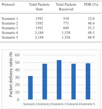
PACKET DELIVERY RATIO (PDR)
The data packet delivery ratio is the ratio of the number of packets received at the destination to the number of packets generated at the source. Table 4 shows the number of total packets sent and received for each of the simulated scenarios and a graphical representation of the packet delivery ratio is shown in Figure 6. The packet delivery ratio can be calculated as follows:
Total Packets received
Packet delivery ratio = (1) Total Packets sent
From Figure 6, it is observed that the scenario with the higher number of nodes has a higher packet delivery ratio. This is as a result of the increase in the nodes density, which brings the deployed sensor nodes in a closer range to each other. The farm data can be better routed successfully and hence delivered to the PAN coordinator in the denser than in
the sparse sensor deployment. Comparing Scenario 2 with Scenarios 4 and 5, it can be seen that the packet delivery ratio has little effect on the number of sending CBR applications. Increasing mobile traffic sources causes the PDR to reduce by 0.1%. But for the addition of static traffic sending nodes,
the PDR increases by 0.5%. This means that increasing traffic
from mobile nodes reduces the PDR, while increasing traffic
from static nodes increases the PDR. Therefore, the traffic
from static sensor nodes can be said to provide higher PDR than traffic from mobile sensor nodes.
AVERAGE END-TO-END DELAY
This metric is calculated by subtracting time at which the
first packet was transmitted by the source from the time at which the first data packet arrived at the destination. This
includes all possible delays caused by buffering during route discovery, queuing at the interface queue, retransmission delays at the MAC, propagation and transfer times. Figure 7
shows a graphical representation of the average end-to-end for the simulated smart farm scenarios.
The average end-to-end delay result for scenarios 1, 2 and 3 does not change proportionately as the number of nodes is increased as shown in Figure 7. The second and third scenarios with the second and third highest number of nodes have the second and third highest average end-to-end
TABLE 4. Total Packets Sent and Received
Protocol Total Packets Total Packets PDR (%) Sent Received Scenario 1 1592 510 32.0 Scenario 2 1592 771 48.4 Scenario 3 1592 849 53.3 Scenario 4 3,184 1,538 48.3 Scenario 5 3,184 1,556 48.9
FIGURE 6. Packet delivery ratio
delay respectively. It is expected that the average end-to-end delay increases as the number of nodes is increased due to
packets queueing and buffer overflow at the relay nodes and sink node. The first scenario, however, which has the lowest
number of nodes has the highest delay. From the PDR result
in Figure 6, it can be concluded that the irregular higher delay encountered in Scenario 1 due to the considerably low PDR,
which results in retransmission delays. Furthermore, it can be seen that the addition of CBR from mobile nodes (Scenario 4) increases the average end-to-end delay by significantly high
value. This implies that increasing nodes mobility causes an increase in the average end-to-end delay. For the addition of CBR from static nodes as in Scenario 5, there is also an
increase in the average end-to-end delay but with a minimal value of fewer than 0.01 seconds.
FIGURE 7: Average end-to-end delay AVERAGE JITTER (SECONDS)
Average jitter is the average values of the variations in the inter-arrival time of packets at the destinations. Figure 8 shows the average jitter of different nodes placement based on their number in the farm environment.
FIGURE 8: Average Jitter
From Figure 8, the simulation results 0.004 of Scenarios 1, 2 and 3 shows that the average jitter increases as the number of nodes increase. Network congestion generally causes jitter (Pucha et al. 2007) which increased as the number of nodes
is increased. The results for the average jitter in Scenarios 4 and 5 follows almost a similar trend with that of the average end-to-end delay. Addition of CBR from mobile nodes in
Scenario 4 increases the average jitter by high value. This is also an indication that increasing nodes mobility causes the average jitter to increase. For the addition of static nodes in Scenario 5, there is a little increase of less than 0.2 seconds in the average jitter value.
TOTAL CONSUMED ENERGY
This is the total consumed energy during the simulation. Figure 9 shows the results for the total consumed energy under the MICAz energy model. The total consumed energy increased as the number of nodes is increased. As the traffic
sources are increased in Scenarios 4 and 5 as compared to Scenario 2, the total consumed energy also increases with almost similar values for the increase in mobile and static sources but mobile being slightly higher. This implies that mobile nodes have higher energy consumption than static nodes.
The receiver and transmitter parts of the transceiver are active in ‘receive’ and ‘transmit’ modes respectively. In ‘idle’ mode, the nodes consume power but are neither transmitting nor receiving any data between them. The ‘sleep’ mode is the energy consumption while the radio is completely turned off and no power is used.
The results of the ‘transmit’ and ‘receive’ modes energy consumption show that for all the three energy models, the consumed energy increases proportionately as the number of nodes increases. However, the energy consumption in ‘receive’ mode is always higher than the ‘transmit’ mode consumption. This is because of the deployment of more sophisticated demodulation schemes which makes reception dominates in terms of energy consumption (Akyildiz et al. 2010).
For the ‘idle’ and ‘sleep’ modes, the energy consumption does not follow a regular pattern in terms of increase in a number of nodes. For the ‘idle’ mode it has the highest consumption in 40 nodes size and lowest in 30 nodes size, while the ‘sleep’ mode stays at zero for all except in MICA
energy model, where it slightly changes when the number of nodes is changed.
The Generic energy model has the highest energy consumption in all three nodes size in ‘receive’ and ‘transmit’ modes followed by MICAz and then MICA models. In ‘idle’
mode, the Generic model consumed the highest amount of energy followed by MICA and MICAz models. A very
high amount of energy is consumed in all the smart farm
scenarios in the ‘idle’ mode, specifically the Generic model.
This is because of its consideration of reception power as the ‘idle’ power. The energy consumption during the ‘idle’ period should be a major concern in the smart farm since monitored data from the environment is less frequently sent by the sensor devices, and hence the long idle duration will affect the overall battery life of the farm sensor nodes. In ‘sleep’ mode, the MICA energy model has a slightly higher
consumption (about 0.03 mWh) while the others consumed 0 mWh. Increasing the sleep time in the smart farm will conserve a lot of energy (up to 100%) depending on the sleep duration. For the overall consumed energy, the Generic model has the highest total consumed energy and MICAz model has
the least.
CONCLUSION AND FUTURE WORK
In this paper, five smart farm deployment scenarios
with wireless ZigBee mesh network topology have been developed and evaluated. The results proof that there is an increase in throughput and packet delivery ratio as the nodes density increases. Increasing CBR initiating from mobile
sources causes the total consumed energy, overall network throughput, average end-to-end delay and average jitter to be higher than the static sources. However, the packet delivery
ratio is slightly higher when more static traffic sending
nodes is present than the mobile sending nodes. Highest total consumed energy is from the Generic radio energy model and
ENERGY MODELS ANALYSIS
The graphic representation of the energy models simulation result for ‘receive’ (Rx), ‘transmit’ (Tx), ‘idle’ and ‘sleep’ modes are shown in Figure 10 under three different node size.
FIGURE 9: Total consumed energy under MICAz energy model
4.5 4 3.5 3 2.5 2 1.5 1 0.5 0 (mWh)
Scenario 1 Scenario 2 Scenario 3 Scenario 4 Scenario 5
Sleep mode Tx mode Rx mode Idle mode
FIGURE 10: Energy consumption based on Generic, MICAz and
mica models for different nodes size
35 30 25 20 15 10 5 0 (mWh)
Scenario 1 Scenario 2 Scenario 3
Generic Generic
Generic
MICAZ MICA MICAZ MICA MICAZ MICA
Sleep mode Tx mode Rx mode Idle mode
lowest is in the MICAz radio energy model. The MICAz has
the lowest ‘Idle’ and ‘receive’ modes consumption as well as the total consumed energy as compared with the other energy models in all the three scenarios investigated. As such, MICAz
is found to be the most suitable energy model that can be applied in the future smart farm deployment.
To further explore the energy consumption in the smart
farm, different traffic application and routing protocols
can be considered. The energy models can also be further evaluated for different wireless sensor networks application. Furthermore, protocols that minimize the idle period and
increases sleep time should be developed to significantly
reduce energy consumption in the wireless sensor nodes.
REFERENCES
Horton M., Culler D., Pister K., Hill J., Szewczyk, R. & Woo, A. 2002. MICA: The Commercialization of Microsensor Motes. Sensors. http://www.sensorsmag. com/articles/0402/40/main.shtml.
Alexandratos, N. & Bruinsma, J. 2012. World agriculture towards 2030/2050: The 2012 revision. FAO ESA Working Paper No. 12-03.
Watthanawisuth, N., Tuantranont, A. & Kerdcharoen, T. 2009. Microclimate real-time monitoring based on ZigBee sensor network. IEEE Sensors Conference 1814-1818. Jawad, H., Rosdiadee, N., Sadik G., Aqeel, J. & Mahamod,
I. 2017. Energy-efficient wireless sensor networks for
precision agriculture: A review. Sensors 17(8): E1781. Murugan, D., Garg, A. & Singh, D. 2017. Development of an
adaptive approach for precision agriculture monitoring with drone and satellite data. IEEE Journal of Selected Topics in Applied Earth Observations and Remote Sensing 10(12): 1-7.
Bacco, M., Andrea, B., Alberto, G. & Luca, C. 2018. IEEE 802.15.4 Air-Ground UAV Communications in smart farming scenarios. IEEE Communications Letters 22(9): 1910-1913.
Norshahkilla, Z., Othman, K. & Nurul Afina, A. 2016. Water
quality of surface runoff in loop two catchment area in UKM. Jurnal Kejuruteraan 28: 65-72.
Maurya, S. & Vinod Kumar Jain. 2017. Energy-efficient
network protocol for precision agriculture. IEEE Consumer Electronics Magazine 6(3): 42-51.
Jawad, H., Rosdiadee, N., Sadik, G., Aqeel, J. & Mahamod, I. 2018. Power reduction with sleep/wake on redundant data (SWORD) in a wireless sensor network for
energy-efficient precision agriculture. Sensors 18(10): 3450. Scalable Network Technologies Inc., QualNet 4.5.1 Wireless
Model Library 2008. [online]. https://www.cs.ucsb. edu/~ebelding/courses/284/qualnet/QualNet-4.5.1-Wireless-ModelLibrary.pdf.
Crossbow Technology, Inc, MICA Wireless Measurement System data sheet, Document Part Number: 6020-0041-01. 2003. https://www.willow.co.uk/MICA.pdf
Crossbow Technology, Inc., MICAz Wireless Measurement System data sheet, Document Part Number:
6020-0103-02 Rev A. 2012. https://www.willow.co.uk/MICAz_ OEM_Edition_Datasheet.pdf
Rohini, S. & Lobiyal, D. K. 2015. Energy based proficiency
analysis of ad-hoc routing protocols in wireless sensor networks. International Conference on Advances in Computer Engineering and Applications (ICACEA). 882-886.
Sarah, A. & Sanjeet, K. 2014. Performance of wireless sensor network under various energy models, routing protocols and node mobility conditions. International Conference on Advanced Communication Control and Computing Technologies (ICACCCT). 813-817.
Sarvesh, K. S., Rajeev, P., Shiv, Veer S. R. & Tanbeer, K. 2014 Analysis of energy model and QoS in wireless sensor network under different modulation schemes. IEEE International Conference for Convergence of Technology (I2CT). 1-5.
Jabbar, W. A., Ismail, M. & Nordin, R. 2015. Multi-criteria based multipath OLSR for battery and queue-aware routing in multi-hop ad hoc wireless networks. Wireless Networks 21(4): 1309-1326.
MacDonald, J. M., Penni, K., & Robert, A. H. 2013. Farm Size and the Organization of U.S. Crop Farming ERR-152. U.S. Department of Agriculture, Economic Research Service.
Kuzminykh, I., Snihurov, A. & Carlsson, A. 2017. Testing of Communication Range in ZigBee Technology. 2017 14th International Conference on the Experience of Designing and Application of CAD Systems in Microelectronics (CADSM). 133-136.
Grossglauser, M. & Tse, D. 2002. Mobility increases the capacity of ad hoc wireless networks. IEEE/ACM Transactions on Networking 10(4): 477-486.
Pucha, H., Zhang, Y., Mao, Z. M. & Hu, Y.C. 2007. Understanding network delay changes caused by routing events. Proceedings of SIGMETRICS'07, San Diego, California 35(1): 73-84.
Akyildiz, I. F. & Mehmet, C. V. 2010. Wireless Sensor Networks. Wiley Publication.
*Hilal Bello Sa’id
Department of Information and Communication Technology, Faculty of Engineering and Environmental Design, Usmanu Danfodiyo University Sokoto, Nigeria. Rosdiadee Nordin, Nor Fadzilah Abdullah
Centre of Advanced Electronic & Communication Engineering, Faculty of Engineering and Built Environment, Universiti Kebangsaan Malaysia 43600, Bangi, Malaysia. *Corresponding author; email: