www.hydrol-earth-syst-sci.net/19/2163/2015/ doi:10.5194/hess-19-2163-2015
© Author(s) 2015. CC Attribution 3.0 License.
Implementation and validation of a Wilks-type multi-site daily
precipitation generator over a typical Alpine river catchment
D. E. Keller1,2,3, A. M. Fischer1, C. Frei1, M. A. Liniger1,3, C. Appenzeller1,3, and R. Knutti2,3
1Federal Office of Meteorology and Climatology MeteoSwiss, Operation Center 1, 8085 Zurich-Airport, Switzerland 2Institute for Atmospheric and Climate Science, ETH Zurich, Universitaetstrasse 16, 8092 Zurich, Switzerland 3Center for Climate Systems Modeling (C2SM), ETH Zurich, Universitaetstrasse 16, 8092 Zurich, Switzerland
Correspondence to: D. E. Keller ([email protected])
Received: 27 June 2014 – Published in Hydrol. Earth Syst. Sci. Discuss.: 28 July 2014 Revised: 23 March 2015 – Accepted: 25 March 2015 – Published: 6 May 2015
Abstract. Many climate impact assessments require high-resolution precipitation time series that have a spatio-temporal correlation structure consistent with observations, for simulating either current or future climate conditions. In this respect, weather generators (WGs) designed and cali-brated for multiple sites are an appealing statistical down-scaling technique to stochastically simulate multiple real-isations of possible future time series consistent with the local precipitation characteristics and their expected future changes. In this study, we present the implementation and validation of a multi-site daily precipitation generator re-built after the methodology described in Wilks (1998). The gener-ator consists of several Richardson-type WGs run with spa-tially correlated random number streams. This study aims at investigating the capabilities, the added value and the limita-tions of the precipitation generator for a typical Alpine river catchment in the Swiss Alpine region under current climate. The calibrated multi-site WG is skilful at individual sites in representing the annual cycle of the precipitation statis-tics, such as mean wet day frequency and intensity as well as monthly precipitation sums. It reproduces realistically the multi-day statistics such as the frequencies of dry and wet spell lengths and precipitation sums over consecutive wet days. Substantial added value is demonstrated in simulat-ing daily areal precipitation sums in comparison to multiple WGs that lack the spatial dependency in the stochastic pro-cess. Limitations are seen in reproducing daily and multi-day extreme precipitation sums, observed variability from year to year and in reproducing long dry spell lengths. Given the per-formance of the presented generator, we conclude that it is a useful tool to generate precipitation series consistent with
the mean climatic aspects and likely helpful to be used as a downscaling technique for climate change scenarios.
1 Introduction
In Switzerland, precipitation is a key weather variable with high relevance for sectors such as energy production, infras-tructure, tourism, agriculture and ecosystems. Owing to a complex topography, daily precipitation varies strongly in space and time (Frei and Schär, 1998; Isotta et al., 2013). The spatial distribution of daily precipitation frequency and intensity depends on the topography, with higher frequen-cies and intensities along the northern Alpine ridge during summer, and a strong north–south gradient with heavier in-tensities in southern Switzerland from spring to autumn. The most prominent weather situations causing these precipita-tion patterns are shallow pressure systems favouring convec-tive precipitation, orographically induced precipitation (e.g. föhn situations), and frontal passages. Precipitation amounts and frequencies are typically largest in summer, mainly due to convective processes (Frei and Schär, 1998).
pre-cipitation change data derived from regional climate mod-els by the well-known and simple delta change approach, which shifts an observed time series by a model-derived change in the mean climate (BAFU, 2012; Bosshard et al., 2011; CH2014-Impacts, 2014). The delta change approach accounts for changes in the mean annual cycle, but potential changes in inter-annual variability, and changes in wet day frequency and intensity or of spell lengths are not taken into account. Hence, the data are also not suitable for the analysis of future changes in extreme events (Bosshard et al., 2011). It is our aim here to develop a statistical downscaling method for Switzerland that overcomes some of these limitations and that subsequently can be easily applied to climate model out-put.
Over recent years a vast number of statistical downscal-ing methods have been developed that go far beyond a sim-ple delta change approach (Maraun et al., 2010). These in-clude bias-correction methods (e.g. Themeßl et al., 2011), regression-based methods (e.g. Hertig and Jacobeit, 2013) or weather generator (WG) approaches (e.g. Chandler and Wheater, 2002; Mezghani and Hingray, 2009). For our pur-poses, the latter method is especially appealing, since it in-cludes a stochastic component. This is a major improvement compared to a (deterministic) delta change approach, allow-ing us to investigate multiple time series and uncertainty at the local scale that are consistent with a given (current or future) mean climate. Moreover, it allows the incorporation of changes in the temporal correlation structure and conse-quently alterations of the dry–wet sequences. From an agri-cultural impact (e.g. Calanca, 2007) or water resource man-agement (e.g. Samuels et al., 2009) perspective, this is a key aspect of future precipitation change.
A serious limitation of many WGs is that they are often calibrated to observations at single sites only, thereby lacking the spatial correlation structure that is required for many ap-plications, particularly in the context of hydrological impact modelling in a topographically complex terrain such as the Alps. A number of sophisticated approaches in time–space precipitation simulation have been put forward in the liter-ature to address this issue, such as K-nearest neighbour re-sampling approaches (e.g. Buishand and Brandsma, 2001), copula-based approaches (e.g. Bárdossy and Pegram, 2009), Poisson cluster models (e.g. Cowpertwait, 1995; Fatichi et al., 2011) or more sophisticated field generators (e.g. Paschalis et al., 2013; Peleg and Morin, 2014). Of increas-ing popularity are Markovian multi-site models (e.g. Baig-orria and Jones, 2010; Wilks, 1998) and in particular non-homogeneous hidden Markov models (NHMMs) (e.g. Bel-lone et al., 2000; Hughes et al., 1999; Kioutsioukis et al., 2008; Robertson et al., 2004, 2009). The latter approach models transitions between pre-defined precipitation state patterns conditional on the synoptic-scale circulation. Each of these time–space WGs come with method-specific bene-fits and limitations for the reproduction of the daily precipita-tion statistics and consequently its use in impact models. For
instance, some of them do better in simulating more realis-tically longer-term variability (e.g. generalised linear model (GLM) based multi-site WGs, Chandler, 2014), while some are explicitly adapted to deal with extreme precipitation (e.g. Huser and Davison, 2014).
The main purpose of our precipitation generator is its use as a downscaling tool in a climate change context. It should be easily transferable to different climatological re-gions and time periods and its generated time series should serve several impact applications that have different needs in terms of time–space consistency. For these reasons we opt for a precipitation generator whose degree of complex-ity and associated calibration requirements are still suffi-ciently easy to handle. Mehrotra et al. (2006) inter-compared three stochastic multi-site precipitation occurrence tors over a region over Australia and found that the genera-tor by Wilks (1998) outperforms hidden Markov models and K-nearest neighbour resampling techniques in terms of over-all performance, time required for model running and sim-plicity of the model structure. Hence the multi-site precip-itation generator proposed by Wilks (1998) serves our pur-poses. It is a relatively simple tool based on a Richardson-type WG (Richardson, 1981) run with spatially correlated random number streams.
It is the aim of this study to investigate the capabilities, the added value and the limitations of this multi-site generator in order to better interpret the climatic changes in the simulated time series for a future climate, which is part of an upcom-ing study. In particular, the actual amount of stochastically generated variability will be assessed as well as the added value of a multi-site model against multiple single-site mod-els. The analysis is done for Swiss catchment Thur. While not being of the same level of familiarity as other catchments, the Thur catchment serves as an ideal test bed for our purposes, as will be detailed in Sect. 2. In Sect. 3 we recapitulate the basic procedures for multi-site precipitation simulation af-ter Wilks (1998) and detail how the generator was calibrated over the catchment. Results of the validation against obser-vations and against single-site generators will be presented in Sect. 4. We end the article with a discussion (Sect. 5) and a summary and outlook (Sect. 6).
2 Selection of the catchment area
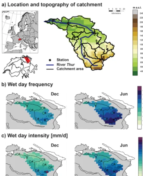
Figure 1. (a) The catchment of the river Thur, located in north-eastern Switzerland, together with the underlying topography (in m a.s.l.). The dots indicate the locations of the investigated sta-tions. 1: Andelfingen (AFI, 47.60◦N, 8.69◦E); 2: Frauenfeld (FRF, 47.57◦N, 8.89◦E); 3: Bischofszell (BIZ, 47.50◦N, 9.23◦E); 4: Eschlikon (EKO, 47.45◦N, 8.97◦E); 5: Ebnat-Kappel (EBK, 47.27◦N, 9.11◦E); 6: Herisau (HES, 47.39◦N, 9.26◦E); 7: Appen-zell (APP, 47.34◦N, 9.40◦E); 8: Saentis (SAE, 47.25◦N, 9.34◦E). The polygons represent sub-catchments. (b) Observed precipitation climatology of the wet day frequency (1961–2011) derived from a 2.2 km×2.2 km gridded daily precipitation data set (Frei and Schär, 1998) for December and June. The grey polygons represent the north-eastern part of the Swiss territory. (c) The same as in (b) but for wet day intensity (in mm day−1). A wet day is defined as a day with a precipitation amount equal to or higher than 1 mm day−1. The filled circle symbols point to the station locations (as in (a)) together with the observed station measurements.
snow at higher stations in the mountains, whereas in the low-lands less than 10 % of the annual sums fall as snow. This particular catchment was selected for mainly two reasons.
1. In an upcoming study our generated synthetic time se-ries over the Thur catchment will serve as input to two hydrological models to assess the runoff regime under current and future climates (similar to in Jasper et al., 2004). The Thur is a well-studied and well-observed river catchment in Switzerland (e.g. Fundel et al., 2013; Kunstmann et al., 2006) providing high-quality hydro-logical measurement series for a robust calibration of hydrological runoff models. It further represents the
largest Swiss river without a natural or artificial reser-voir and therefore exhibits discharge fluctuations simi-lar to unregulated Alpine rivers.
2. Owing to the complex topography over this catchment area (ranging from less than 400 m a.s.l. to more than 2500 m a.s.l.), precipitation exhibits a large variability both in space and in time (see Fig. 1b and c based on gridded observational data from Frei and Schär, 1998). Over 1961–2011 and for a winter and summer month, the data clearly show larger precipitation frequencies and intensities over higher-elevated regions compared to the lowlands. A large portion of these precipitation characteristics can be explained by a north-east to south-west lying mountain range (Alpstein) extracting precip-itation from westerly flows and triggering convective storms. These spatio-temporal variations hence serve as an ideal observation basis to validate and analyse the capabilities and limitations of the WG.
For the purpose of this study, we selected eight evenly dis-tributed measurement stations (Fig. 1a) of MeteoSwiss that all provide homogenised time series covering a 51-year pe-riod from 1961 to 2011 (Begert et al., 2003), and that suffi-ciently cover the elevation profile of the catchment area.
3 Method
3.1 Precipitation occurrence and amount model The core of our multi-site WG is a Richardson-type pre-cipitation generator (Richardson, 1981) consisting of an oc-currence and amount model. To model ococ-currence at a sin-gle station we rely on a first-order two-state Markov chain (Gabriel and Neumann, 1962; Richardson, 1981; Wilks and Wilby, 1999). The use of a first-order model in our WG was justified by inspecting the Akaike information crite-rion (AIC) (Akaike, 1974) and the Bayesian information criterion (BIC) (Schwarz, 1978). Both criteria revealed a substantial improvement when going from a zero-order to first-order model, but the additional gain at a second- or higher-order model was negligible (not shown). We used a specific wet day threshold of 1 mm day−1 to discretise a given daily precipitation time seriesX(t )at a given site into the two states “dry” (X(t ) <1 mm day−1,J
t=0) and “wet”
(X(t )≥1 mm day−1, J
t=1). The wet–wet (p11) and dry– wet (p01) transition probabilities suffice to fully specify the first-order two-state Markov chain model.
For an estimate of the transition probabilities, we rely on their conditional relative frequencies (Wilks, 2011). Other important precipitation indices can be inferred. The wet day frequency (wdf,π) is defined as the ratio of the number of wet days to the total number of days over a given time pe-riod:
π= p01
1+p01−p11
[image:3.612.50.286.65.354.2]Similarly, the lag-kautocorrelationrkis defined as
rk=(p11−p01)k. (2)
Since day-to-day precipitation generally exhibits positive se-rial correlation (i.e.r1>0),p11is usually larger thanp01and the wdf is between the two. Note that a first-order Markov chain does not imply independence for lags greater than 1. The autocorrelation rk (Eq. 2) decays exponentially with
larger lagsk.
Given a simulated wet day from the occurrence model, precipitation amounts are set. This is done by sampling from a mixture model of two exponential distributions (Wilks, 1999a):
f (x)= w
β1
exp
−x
β1
+1−w
β2
exp
−x
β2
. (3)
f (x) is a weighted average (weightw)of two exponential
distributions with means β1 andβ2. The parameters w,β1 andβ2are estimated based on maximum likelihood (Tallis and Light, 1968). Note that the estimation of PDF parameters is subject to sampling uncertainty from the available number of wet days in a given calendar month.
3.2 Stochastic modelling of multi-site daily precipitation
The simulation process is based on Richardson (1981) at sin-gle stations with the five above-introduced parameters, i.e. the transition probabilitiesp11andp01as well asw,β1and
β2. That is, a uniform random number between 0 and 1 is compared to eitherp11 orp01, depending on the state of the previous day, and correspondingly set as either dry or wet. In the case of a wet day, a second uniform random number is drawn to assign the precipitation amount based on the quan-tile function. For further details on the simulation of precip-itation at a single location, we refer the reader to Wilks and Wilby (1999) and to the Supplement. The simulation allows time series of arbitrary lengths resembling observed clima-tological precipitation statistics, in terms of both frequency and intensity.
The main extension to a multi-site model after Wilks (1998) is to drive several single-site WGs simul-taneously with spatially correlated but serially independent random numbers. To generate correlated random number streams, we rely on a Cholesky decomposition (e.g. Higham, 2009). The latter requires matrices that are positive definite, which is not always granted. In their absence, a fall-back solution based on the nearest positive correlation matrix is chosen (e.g. Higham, 1989). This problem, however, occurs only a few times in our study. One of the main hurdles in simultaneously generating precipitation at multiple sites is to ensure that the spatial dependence is also preserved in the final generated time series (Wilks and Wilby, 1999; Wilks, 1998). This difficulty mainly arises from the stochastic
process that partly destroys the initially imposed correlation structure again (Wilks, 1998). To circumvent this problem, Wilks (1998) suggested an optimisation procedure based on a bisection method (Burden and Faires, 2010) that minimises the difference between the generated spatial correlation and the target correlation of observations. In our case, the iteration is repeated until a precision of 0.005 is reached. This estimation procedure is done prior to the actual simulation and has to be done for each station pair and each month. For further details regarding the set-up of stochastic simulation and in particular the implementation of multi-site simulation, we refer the reader to the Supplement.
3.3 Implementation
3.3.1 Implementation of the multi-site WG over the Thur catchment
The precipitation generator is calibrated on a monthly basis. First, all the single-site input parameters (p11,p01,β1,β2 andw) were estimated for each of the eight stations within the catchment and for each month separately using a time window of 51 years (1961–2011). In this study we chose a relatively long calibration period in order to minimise the ef-fect of sampling uncertainties. This allows us to accurately assess the added value of a multi-site model against multiple single-site models and to better quantify systematic biases of the WG. For the two transition probabilities in a given month, the climatological mean over the 51 yearly values ofp11and
re-● ●
● ●
0.0 0.2 0.4 0.6 0.8 1.0 0.0
0.2 0.4 0.6 0.8 1.0
Wet day frequency
INPUT
MODEL
Sample size 10000 1000 100 30 Sample size
10000 1000 100 30
● ●
●
●
0 5 10 15 20
0 5 10 15 20
Wet day intensity [mm]
INPUT
MODEL
● ●
● ●
0.0 0.2 0.4 0.6 0.8 1.0 0.0
0.2 0.4 0.6 0.8 1.0
Wet−wet transition probability
INPUT
MODEL
● ●
● ●
0.0 0.2 0.4 0.6 0.8 1.0 0.0
0.2 0.4 0.6 0.8 1.0
Dry−wet transition probability
INPUT
[image:5.612.51.288.66.303.2]MODEL
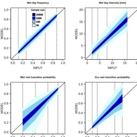
Figure 2. Reproduction of average wet day frequency (wdf), mean wet day intensity (wdi), wet–wet transition probability (p11) and
dry–wet transition probability (p01) for the four idealised climate
regimes ranging from very dry (left) to very wet (right) as indicated by dashed lines. The shaded areas correspond to the range between the 2.5 and 97.5 % empirical quantiles of 100 realisations. Results are shown for sample sizes of 10 000, 1000, 100 and 30 (grey shad-ing).
sults presented in Sect. 4 are calculated over the time period 1961–2011.
3.3.2 Reproduction and uncertainty of WG model parameters
To test whether our WG is properly implemented, we evalu-ated the reproduction of WG input parameters extracted from the generated time series. A correct reproduction in parame-ters such as wet day intensity, frequency and transition prob-abilities is a prerequisite for all the subsequent analyses pre-sented in Sect. 4. The evaluation was performed for four sub-jectively defined climatic regimes: a very dry, a dry, a wet and a very wet climate. The corresponding model parameters are indicated in Fig. 2 with dashed vertical lines. For each of these precipitation regimes, 100 synthetic daily time series were generated. To test the effect of sample size, different sizes of time windows were used: (a) 10 000 days, (b) 1000 days, (c) 100 days and (d) 30 days. The latter corresponds to the same sample size as for the simulation of precipitation occurrence over the Thur catchment. For each of the gener-ated time series, the WG parameters were re-estimgener-ated and the 95 % inter-quantile range was computed across the set of 100 realisations (Fig. 2). Three main results can be in-ferred: (a) our precipitation generator is able to correctly
re-produce the key WG parameters, implying that the chances of substantial coding errors are small. (b) As expected, the estimate of the input parameters becomes more uncertain for smaller sample sizes; in fact, the uncertainty range in-creases by a factor of 18.3 when the sample size is reduced from 10 000 to 30. At a sample size of 1000, the uncertainty range stays at around±0.03, which is only marginally low-ered when going to a sample size of 10 000. (c) The different pre-defined climate regimes affect the uncertainty, particu-larly in the estimated transition probabilities. In a very dry or wet climate, the wet–wet or dry–wet transition probabil-ity, respectively, exhibits large uncertainties in the estimate. This again is mainly related to a sample size problem due to very few wet–wet or dry–wet pairs. Thus, we expect that the weather generator will not work optimally in extremely wet or arid climates.
4 Results
An in-depth evaluation of the generated time series with our calibrated multi-site WG is now undertaken with real ob-servations. First, the reproduction of the daily and longer-term precipitation statistics at individual sites is analysed (Sect. 4.1). In a second step, the performance of the multi-site model is investigated regarding spatially aggregated precip-itation indices in comparison to WGs without incorporating spatial dependencies (Sect. 4.2).
4.1 Validation of the precipitation generator at individual sites
Based on our ensemble of synthetic time series, each con-taining 51 years, we analyse the reproduction of key precip-itation characteristics. This validation goes beyond the re-production of pure model parameters used to calibrate the WG (Sect. 3.3.2), as it includes precipitation statistics that are not directly used in the specification and calibration of the model. Note that we present this analysis for the same time period as used for calibrating our WG. This is justified for the study here, as long as we treat and use our WG to simulate long-term monthly precipitation statistics. In such a set-up, the stationarity of the model is given by definition. However, in a climate prediction or projection context, this stationarity assumption would have to be tested, and hence separate calibration and validation periods are needed. 4.1.1 Long-term mean and inter-annual variance of
monthly precipitation sums
● ● ● ● ● ● ● ● ● ● ● ● 20 40 60 80 100 120
Monthly sums [mm]
● ● ● ● ● ● ● ● ● ● ● ● ● ● ● ● ● ● ● ● ● ● ● ●
J F M A M J J A S O N D
34 24 28 26 32 38 42 46 40 32 27 29 AFI ● ● ● ● ● ● ● ● ● ● ● ● 50 100 150 200 250
Monthly sums [mm] ● ● ● ● ● ● ● ● ● ● ● ● ● ● ● ● ● ● ● ● ● ● ● ●
J F M A M J J A S O N D
28 21 34 33 34 45 32 46 43 49 29 26 APP ● ● ● ● ● ● ● ● ● ● ● ● 20 40 60 80 100 120 140
Monthly sums [mm]
● ● ● ● ● ● ● ● ● ● ● ● ● ● ● ● ● ● ● ● ● ● ● ●
J F M A M J J A S O N D
77 62 59 41 40 54 46 47 34 50 30 38 BIZ ● ● ● ● ● ● ● ● ● ● ● ● 50 100 150 200 250
Monthly sums [mm]
● ● ● ● ● ● ● ● ● ● ● ● ● ● ● ● ● ● ● ● ● ● ● ●
J F M A M J J A S O N D
24 18 22 31 41 46 32 44 35 40 27 25 EBK ● ● ● ● ● ● ● ● ● ● ● ● 40 60 80 100 120 140 160
Monthly sums [mm]
● ● ● ● ● ● ● ● ● ● ● ● ● ● ● ● ● ● ● ● ● ● ● ●
J F M A M J J A S O N D
29 23 31 33 33 44 37 50 32 39 24 28 EKO ● ● ● ● ● ● ● ● ● ● ● ● 40 60 80 100 120 140 160
Monthly sums [mm]
● ● ● ● ● ● ● ● ● ● ● ● ● ● ● ● ● ● ● ● ● ● ● ●
J F M A M J J A S O N D
35 22 33 32 32 40 48 42 39 37 27 28 FRF ● ● ● ● ● ● ● ● ● ● ● ● 50 100 150 200
Monthly sums [mm]
● ● ● ● ● ● ● ● ● ● ● ● ● ● ● ● ● ● ● ● ● ● ● ●
J F M A M J J A S O N D
50 33 33 39 37 46 41 49 39 45 43 53 HES ● ● ● ● ● ● ● ● ● ● ● ● 100 150 200 250 300 350
Monthly sums [mm]
● ● ● ● ● ● ● ● ● ● ● ● ● ● ● ● ● ● ● ● ● ● ● ●
J F M A M J J A S O N D
[image:6.612.113.485.62.422.2]24 23 20 22 29 38 32 31 39 34 28 17 SAE
Figure 3. Long-term mean and variability of monthly precipitation sums during the period 1961–2011 for eight stations in the Thur catch-ment. The black (blue) lines refer to the mean annual cycle of observed (modelled) precipitation sums. The grey (blue) shaded areas repre-sent the inter-quartile ranges of observed (simulated) monthly precipitation sums. The simulation comprises 100 realisations covering every 51 years. The numbers at the bottom indicate for each month the percentage of variance explained by the precipitation generator. Note that the scale of the y-axis differs between different stations.
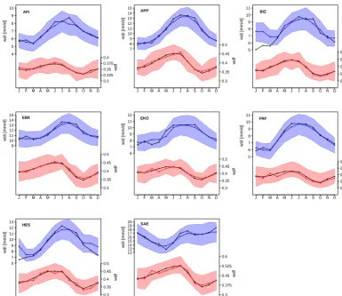
also true of the long-term seasonal as well as for the an-nual precipitation sums (not shown). But, the WG tends to slightly underestimate precipitation sums in June and Au-gust, and overestimate them in October. In addition, the two stations Bischofszell (BIZ) and Herisau (HES) show rather large positive deviations from the observed record during the winter months. In order to explain part of these deviations, we decomposed the long-term mean of monthly (T =30 days) precipitation sums (E[S(T )]) into the product of the mean monthly wet day frequency (wdf) and intensity (wdi) (Fig. 4):
E[S (T )]=T·wdf·wdi. (4)
Since these two climatological quantities are indirectly forced (Sect. 3.3.2), we expect from the results in Fig. 2 a good match on average. As shown in Fig. 4, this is true for the wet day frequency, where the deviations between gen-erated (red) and observed (black) values are relatively small.
The differences, however, are more pronounced in the case of mean wet day intensities. In fact, it is the wet day intensities that explain the mismatches in precipitation sums. In case of the winter performance over Bischofszell and Herisau, the deviations can be attributed to the failure of converg-ing in the case of fittconverg-ing the non-zero precipitation amount. For those instances, the fallback solution had to be used (see Sect. 3.3.1).
re-● ● ● ● ● ● ● ● ● ● ● ● ● ● ● ● ● ● ● ● ● ● ● ● ● ● ● ● ● ● ● ● ● ● ● ●
J F M A M J J A S O N D
wdi [mm/d] 4 5 6 7 8 9 10 AFI ● ● ● ● ● ● ● ● ● ● ● ● ● ● ● ● ● ● ● ● ● ● ● ● ● ● ● ● ● ● ● ● ● ● ● ● wdf 0.3 0.325 0.35 0.375 0.4 ● ● ● ● ● ● ● ● ● ● ● ● ● ● ● ● ● ● ● ● ● ● ● ● ● ● ● ● ● ● ● ● ● ● ● ●
J F M A M J J A S O N D
wdi [mm/d] 7 8 9 10 11 12 13 14 15 APP ● ● ● ● ● ● ● ● ● ● ● ● ● ● ● ● ● ● ● ● ● ● ● ● ● ● ● ● ● ● ● ● ● ● ● ● wdf 0.3 0.35 0.4 0.45 0.5 ● ● ● ● ● ● ● ● ● ● ● ● ● ● ● ● ● ● ● ● ● ● ● ● ● ● ● ● ● ● ● ● ● ● ● ●
J F M A M J J A S O N D
wdi [mm/d] 5 6 7 8 9 10 11 BIZ ● ● ● ● ● ● ● ● ● ● ● ● ● ● ● ● ● ● ● ● ● ● ● ● ● ● ● ● ● ● ● ● ● ● ● ● wdf 0.3 0.35 0.4 0.45 0.5 ● ● ● ● ● ● ● ● ● ● ● ● ● ● ● ● ● ● ● ● ● ● ● ● ● ● ● ● ● ● ● ● ● ● ● ●
J F M A M J J A S O N D
wdi [mm/d] 9 10 11 12 13 14 15 EBK ● ● ● ● ● ● ● ● ● ● ● ● ● ● ● ● ● ● ● ● ● ● ● ● ● ● ● ● ● ● ● ● ● ● ● ● wdf 0.3 0.35 0.4 0.45 0.5 ● ● ● ● ● ● ● ● ● ● ● ● ● ● ● ● ● ● ● ● ● ● ● ● ● ● ● ● ● ● ● ● ● ● ● ●
J F M A M J J A S O N D
wdi [mm/d] 6 7 8 9 10 11 12 EKO ● ● ● ● ● ● ● ● ● ● ● ● ● ● ● ● ● ● ● ● ● ● ● ● ● ● ● ● ● ● ● ● ● ● ● ● wdf 0.3 0.35 0.4 0.45 0.5 ● ● ● ● ● ● ● ● ● ● ● ● ● ● ● ● ● ● ● ● ● ● ● ● ● ● ● ● ● ● ● ● ● ● ● ●
J F M A M J J A S O N D
wdi [mm/d] 5 6 7 8 9 10 11 FRF ● ● ● ● ● ● ● ● ● ● ● ● ● ● ● ● ● ● ● ● ● ● ● ● ● ● ● ● ● ● ● ● ● ● ● ● wdf 0.3 0.35 0.4 0.45 0.5 ● ● ● ● ● ● ● ● ● ● ● ● ● ● ● ● ● ● ● ● ● ● ● ● ● ● ● ● ● ● ● ● ● ● ● ●
J F M A M J J A S O N D
wdi [mm/d] 6 7 8 9 10 11 12 13 HES ● ● ● ● ● ● ● ● ● ● ● ● ● ● ● ● ● ● ● ● ● ● ● ● ● ● ● ● ● ● ● ● ● ● ● ● wdf 0.3 0.35 0.4 0.45 0.5 ● ● ● ● ● ● ● ● ● ● ● ● ● ● ● ● ● ● ● ● ● ● ● ● ● ● ● ● ● ● ● ● ● ● ● ●
J F M A M J J A S O N D
[image:7.612.105.490.64.396.2]wdi [mm/d] 12 13 14 15 16 17 18 19 20 SAE ● ● ● ● ● ● ● ● ● ● ● ● ● ● ● ● ● ● ● ● ● ● ● ● ● ● ● ● ● ● ● ● ● ● ● ● wdf 0.3 0.375 0.45 0.525 0.6
Figure 4. Observed and modelled monthly mean wet day intensity (blue) and frequency (red) at eight stations during 1961–2011. The black (coloured) lines indicate the observed (modelled) values. The blue (red) shaded areas correspond to the inter-quartile range across the set of synthetic daily time series. They comprise 100 runs covering every 51 years.
duced variability is expected, as observations are subject to additional sources of variability, which our comparable sim-ple WG is not trained for. The WG is forced with mean ob-served values, varying between months but not between dif-ferent years. The annual cycle is assumed to be stationary, and hence interannual variability, e.g. related to the North Atlantic Oscillation (Hurrell et al., 2003), is missing. Con-sequently, the ratio of simulated to observed variance ac-counts for approximately 33 % on average. The magnitude of this result is consistent with other studies (e.g. Gregory et al., 1993). Further insights can be gained from a de-composition of the variance of monthly (T =30 days) pre-cipitation sums (Var[S(T)]) into the variance of non-zero amount (Var[X≥1 mm day−1]) and the variance of the num-ber of wet days (Var [N(T)]) as proposed by Wilks and Wilby (1999):
Var [S (T )]=T·wdf·VarhX≥1 mm d−1i+Var [N (T )]·wdi2. (5) Since the mean wet day frequency (wdf) and intensity (wdi) are reasonably reproduced, we expect that the reduced vari-ability of monthly precipitation sums will originate from
de-ficiencies in correctly reproducing the inter-annual variabil-ity of the number of wet days and/or of the non-zero amount. One likely reason is the neglect of low-frequency variabil-ity in the WG parameters. It has been shown that physically based models that include large-scale circulation as a pre-dictor could alleviate this problem (Chandler and Wheater, 2002; Furrer and Katz, 2007; Wheater et al., 2005; Yang et al., 2005).
Dry spells
1 3 5 8 12 16 20
0.2 0.4 0.6 0.8 1.0
Frequency
Spell length [days] June
OBS IQR WG Median WG
January
OBS IQR WG Median WG
Wet spells
1 3 5 8 10 14
0.3 0.4 0.5 0.6 0.7 0.8 0.9 1.0
Frequency
Spell length [days]
Dry spells
1 3 5 8 12 16 20
0.2 0.4 0.6 0.8 1.0
Frequency
Spell length [days] June
OBS IQR WG Median WG
January
OBS IQR WG Median WG
Wet spells
1 3 5 8 10 14
0.3 0.4 0.5 0.6 0.7 0.8 0.9 1.0
Frequency
Spell length [days]
Andelfingen (AFI)
[image:8.612.140.454.65.403.2]Saentis (SAE)
Figure 5. Cumulative distribution of the observed and simulated dry (left) and wet (right) spell length frequencies for lowland station Andelfingen (top) and mountain station Saentis (bottom). Results are for January and June during the time period of 1961–2011. The coloured area (line) represents the inter-quartile range (median) of the 100 realisations covering each 51 year long daily time series.
intensities are systematically underestimated at all stations. This issue could be overcome by more sophisticated amount models combining e.g. a gamma with a generalised Pareto distribution (Vrac and Naveau, 2007).
4.1.3 Reproduction of multi-day statistics
While the frequencies of precipitation amounts and the fre-quencies of wet and dry days are realistically simulated, it remains unclear how the WG performs for multi-day spells. For many application studies, this is essential information that requires a specific analysis. Figure 5 displays observed and modelled cumulative frequencies of dry and wet spell lengths at the example of 2 months and 2 stations. The two stations Saentis and Andelfingen are selected for dis-play since they represent the stations with the highest and lowest elevations in the catchment. For both stations a clear seasonal difference in the probability of dry spells toward more short and fewer long dry spells during summer com-pared to winter is found. A plausible explanation are the more intermittent (convective) precipitation systems during
Figure 6. Cumulative distribution functions (CDFs) of multi-day precipitation sums for the three stations Andelfingen (AFI), Appenzell (APP) and Saentis (SAE). The lines represent the CDFs of non-zero precipitation amounts over 1 day (red), over 3 consecutive wet days (green) and over 5 consecutive wet days (blue). Darker and lighter colours refer to observations and simulations, respectively. The observed CDFs have been derived from a 51-year long daily time series between 1961 and 2011, those of the weather generator from 100 realisations of 51-year long daily simulations. Note that the scaling of the horizontal axis differs between different stations.
Given that the frequency of wet spell lengths is realisti-cally simulated, the question arises whether this also holds for multi-day precipitation sums. Multi-day periods of rain is a common phenomenon over Switzerland, especially dur-ing prevaildur-ing weather situations that favour orographic up-lift. We compared observed and simulated cumulative dis-tribution functions (CDFs) of precipitation sums over mul-tiple consecutive wet days (Fig. 6). Overall, we found that the differences between generated and observed time series are largest for the higher quantiles and for long lasting wet spells (5 day wet spells) where the WG tends to underesti-mate large multi-day sums. This reduced skill in simulating longer wet spell sums can be explained by the fact that our WG is only prescribed with the temporal structure of pre-cipitation occurrence but not in amount. In other words, the WG has the memory to realistically reproduce multi-day wet spell lengths (Fig. 5), while the combined analysis of multi-day occurrence and accumulated amount loses this memory again somewhat. Two further noticeable features in Fig. 6 are that intense 1 day precipitation sums are often overesti-mated by the model compared to the observations, while a relatively good match is obtained for 3 day sums. Although the deficiency in correctly simulating multi-day sums of con-secutive wet days is to be expected by construction of the WG, it could be improved by more sophisticated precipi-tation models, such as multi-state Markov chains with dif-ferent probability density distributions conditioned on pre-defined states, as for instance “dry”, “wet”, and “very-wet” (Boughton, 1999; Gregory et al., 1993).
4.2 Performance of spatial precipitation indices Up to this point we evaluated the generator at individual sites only. One of the key issues of this study though is the poten-tial added value of incorporating inter-station dependencies. Similarly as in the previous section, we analyse the perfor-mance first in terms of occurrence-related statistics and
sec-ond in terms of the combined occurrence and amount statis-tics.
4.2.1 Dry and wet spell statistics for the whole catchment
Based on the eight stations in our catchment, with each be-ing either in a wet or dry state on a given day, theoretically 28(=256) different dry–wet patterns in space are possible. In observations, though, it turns out that 70 % of the investi-gated days over 1961–2011 are in fact either completely dry (45 %) or completely wet (25 %), and the remaining 254 dry– wet patterns are subject to far smaller frequencies (around 10−5–10−3%). The pre-dominance of a dry or a wet catch-ment makes sense given that the catchcatch-ment is relatively small and given that precipitation is to a large degree circulation triggered. Analysing the synthetic time series from our multi-site WG reveals an almost perfect match with observations (Table 1), a consequence of prescribing the spatial depen-dency structure in the occurrence process. Indeed, when re-doing the same experiments with multiple single-site WGs without inter-site dependencies, only about 2 % of all days are completely dry in the catchment, and none of the days is simulated as completely wet (Table 1). In a single-site WG set-up, the chances of all stations being dry or wet ultimately depend on the calibrated wet day frequencies at the eight sta-tions that remain below 0.5 in almost all months (see Fig. 4). This implies that the likelihood of dry conditions over the catchment is higher than for wet conditions.
Table 1. Frequencies (given in percent) of a completely wet or dry catchment together with the frequencies of its spell lengths. The observed (OBS) frequencies are calculated over 1961–2011. The multi-site simulated frequencies are given by the mean of 100 runs over 51 years (1961–2011).
Wet catchment Dry catchment
OBS Multi-site Single-site OBS Multi-site Single-site
Overall frequency 25 25 0 45 44 2
Frequencies of spell lengths 1 34.8 34.4 0.0 14.1 17.3 2
2 27.3 29.4 0.0 16.2 20.7 0.0
3 16.7 18.2 0.0 13.0 18.2 0.0
4 11.5 9.7 0.0 10.8 14.1 0.0
5 4.1 4.7 0.0 9.1 10.3 0.0
6 2.7 2.1 0.0 5.9 7.0 0.0
7 0.9 0.9 0.0 7.2 4.7 0.0
8 0.7 0.4 0.0 5.1 3.0 0.0
9 0.6 0.2 0.0 3.5 1.9 0.0
10 0.2 0.0 0.0 3.5 1.2 0.0
that the calibrated multi-site WG not only captures the fre-quencies of spatially aggregated binary series very well, but it also does a surprisingly good job in reproducing multi-day dry/wet spells of the Thur catchment.
4.2.2 Daily non-zero precipitation sums over the catchment
The above findings on the spatio-temporal correlation struc-ture in the occurrence process also give confidence that daily precipitation sums aggregated over the catchment are rea-sonably simulated. To answer this user-relevant question, we first analyse seasonal distributions of single-day precipita-tion area sums over the time period 1961–2011 (Fig. 7). Area sums are defined as the precipitation sum over the eight sta-tions. Note that days with an area sum of zero were excluded from this analysis and are not shown. The observations (grey box plots) show in the median only a weak inter-seasonal variability with somewhat higher sums during summer. The spread in daily precipitation is smallest for winter and spring and largest for summer, owing to the higher extreme precip-itation values observed. Common to all seasons is a distri-bution that is heavily right-skewed, ranging from nearly dry conditions up to about 220 mm day−1. Note that the spread shown here includes variability from year to year but also within the season of the same year.
Compared to observations, the multi-site generator repro-duces well the median of the observed daily areal sums. The relative deviations remain rather small, ranging from−8.5 % in summer to +1.6 % in autumn. Moreover, the multi-site model is able to capture about 95 % of the observed vari-ability in the daily sums, while the single-site WG only ex-plains about 13 %. Even for extreme areal precipitation, the deficiencies are rather small. Contrary to a multi-site model, the areal sum derived from several single-site WGs over the
−0.6 −25.6 −2.2 −18.4 −8.5 −21.6 1.6
0 50 100 150 200 250
−27.9
Daily areal precipitation sums [mm]
DJF MAM JJA SON
[image:10.612.325.526.296.501.2]Seasons
Figure 7. Daily non-zero precipitation sums over the catchment for the four seasons during 1961–2011. Daily precipitation intensity of the eight stations is summed and days with an area sum of zero are excluded. Box plots of observed daily sums (grey), of multi-site simulated time series (blue) and of single-site simulated time series (red) are shown. The WG models were run 100 times over a 51-year time period. The numbers (in percentage) indicated above the cor-responding model represent the relative deviation of the simulated median from the observed median.
catchment (red) systematically underestimates the median, variability and consequently the magnitude of extreme pre-cipitation amounts (Fig. 7). The relative deviations from ob-servations in the median range from −28 % in autumn to
all stations are wet (Sect. 4.2.1). Also, the spatial structure of the precipitation amount is not accounted for.
4.2.3 Annual maximum precipitation sums of consecutive days over the catchment
The previous analysis has revealed a pronounced added value when incorporating spatial dependencies in the stochastic simulation of daily areal precipitation sums over the Thur.
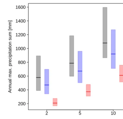
Similarly to Sect. 4.2.1, we want to go a step beyond and additionally include the temporal structure. Note that by in-vestigating spatial precipitation sums over multi-days, we ex-plore the limits of our WG. We analyse in Fig. 8 annual max-ima of observed (grey) and modelled (blue and red for multi-site and single-multi-site, respectively) precipitation sums over sev-eral consecutive days (2, 5, and 10 days). This means that out of the aggregated catchment time series, we compute tem-poral sums over consecutive days and take the maximum in each year.
Regarding the performance of the calibrated WG in multi-site and single-multi-site mode, Fig. 8 shows that both clearly un-derestimate the observed sums. Yet, the multi-site model ex-hibits much smaller deviations from the observed distribu-tion than the single-site model, and hence the added value of the multi-site WG is clearly evident. In fact, the sums simu-lated with the multi-site WG are larger by a factor of around 1.8 than those generated with the single-site WG. Overall, deviations from observations are reduced from about−53 % (single-site WG) to about−17 % (multi-site WG). The added value of the multi-site model is not constant for different consecutive sums. Differences are larger at shorter multi-day sums and decrease toward longer time windows. This is re-lated to the fact that the spatio-temporal correlation structure at longer lags is not prescribed in the model, as already seen in Sect. 4.2.1 and Table 1. The benefit of a multi-site WG in terms of maximum daily areal precipitation sums is therefore restricted to consecutive sums over a few days only. And, as a consequence for time windows of 30 days (or monthly sums), a single-site WG performs equally well as a multi-site WG (not shown), as both models are calibrated for monthly sums at the eight stations and consequently at the catchment.
5 Discussion
The incorporation of inter-station dependencies into the stochastic model brings substantial added value over mul-tiple single-site models regarding daily and multi-day areal precipitation sums over the Thur catchment. Similar benefits from the multi-site WG would be expected for other Alpine catchments and regions with complex topography, where cor-relations between sites are significant but well below unity. For very homogeneous regimes (inter-station correlation near unity), one single-site WG would be sufficient for the
catch-● ●
●
200 400 600 800 1000 1200 1400 1600
Ann
ual max. precipitation sum [mm]
Consecutive Days
[image:11.612.325.527.64.259.2]2 5 10
Figure 8. Annual maximum precipitation summed over all eight stations and over consecutive days. The analysis is done for all days of the year. The bars (horizontal line) indicate the range between the 2.5 and 97.5 % empirical quantiles of the yearly maximum area sums during 1961–2011. The observations are plotted in grey, the multi-site simulations in blue and the single-site simulations in red. The observations comprise 51 years, and the models were run 100 times over a 51-year time period.
ment area, whereas for low spatial correlations, several inde-pendent single-site WGs can be used.
A stochastic simulation with multi-site correlation struc-ture comes with additional uncertainty from parameter es-timations, additional implementation complexity and addi-tional computaaddi-tional costs. The decision for incorporating spatial dependencies must therefore be balanced with the benefit. A careful inspection of the observed precipitation regime and its spatial structure over the catchment prior to the simulation is necessary to decide in favour of or against multi-site simulation. This is also important in terms of vali-dation: for a large catchment area that is frequently affected by frontal passages, the validation of the precipitation gen-erator should include more complex space–time dependency analyses. An example is the probability of a certain precipi-tation amount at a particular sprecipi-tation given precipiprecipi-tation at a neighbouring station some days earlier.
constrained when used as a downscaling technique. How-ever, from model evaluation studies it is well known that climate models are prone to substantial circulation errors (e.g. van Haren et al., 2012; van Ulden and van Oldenborgh, 2006), with effects on the local precipitation. Furthermore, the overall performance of a NHMM is highly dependent on the predictive power of atmospheric circulation patterns and the number of synoptic weather states, respectively (Schie-mann and Frei, 2010). In winter, we would expect a NHMM to perform better than in summer, when the precipitation process is mainly dominated by local-scale convective pro-cesses triggered by orography. However, we need a down-scaling technique that equally applies to all seasons. Also, for a small catchment scale such as the Thur, the variability of the local precipitation pattern is pre-dominantly caused by physiographic factors, such as height differences, or shield-ing effects, rather than by large-scale atmospheric patterns. As was shown in Table 1, at around 70 % of all days over 1961–2011, all stations in the catchment are simultaneously dry or wet. Under these circumstances the use of a NHMM would be feasible after careful calibration. For all these rea-sons, the precipitation generator by Wilks (1998) is in our view the more direct approach to guarantee the spatial con-sistency for the stations in our catchment.
For many impact applications, gridded precipitation data instead of multiple scattered stations would be beneficial. This demand could be achieved by interpolating the spatially consistent synthetic station data over the area of interest. A more sophisticated and elegant method, however, is to build a field generator, for instance by high-dimensional random Gaussian fields (e.g. Pegram and Clothier, 2001), random cascade models (e.g. Over and Gupta, 1996) or Poisson clus-ter models (e.g. Burton et al., 2008). An alclus-ternative would be to rely on geostatistical methods, for instance by prescribing a spatial correlation function at gauged and ungauged loca-tions, which additionally also requires specifying parameters of the WG between the sites (e.g. Wilks, 2009). In regions with complex topography, this additional interpolation is not straightforward. It could be alleviated by explicitly including information on topographic aspects (e.g. altitude, aspect and slope) in a GLM (McCullagh and Nelder, 1989) or Bayesian hierarchical modelling approach (Gelman and Hill, 2006). These are appealing frameworks that allow the modelling of physiographic dependencies in the precipitation amount and occurrence model. However, this alone is not sufficient for a space–time weather generator, as the spatial dependence of daily precipitation is also determined by spatial autocor-relation and not just by the physiographic conditioning of parameters. Clearly, the development of a gridded space– time weather generator dealing with spatial autocorrelation, physiographic conditioning, intermittence and temporal au-tocorrelation is highly challenging and needs fundamental methodological development. This is beyond the scope in the present study, where our main focus was to develop an
easy-to-use statistical downscaling tool for current and future cli-mate.
6 Summary and outlook
The multi-site precipitation generator of Wilks (1998) has been successfully developed, implemented and tested over Swiss Alpine river catchment Thur. The precipitation gener-ator treats precipitation occurrence as a Markov chain and simulates non-zero daily precipitation amounts from a mix-ture model of two exponential distributions. The spatial de-pendency is ensured by running the WG with spatially cor-related random numbers. The model was calibrated on a monthly basis by using daily station data over a 51-year long time period from 1961 to 2011, and extensively compared to the observed record and to simulations based on multiple independent single-site WGs.
Our main findings of this study are the following. – The multi-site precipitation generator realistically
re-produces key precipitation statistics at single stations, including the annual cycle, quantiles of non-zero precip-itation amounts, multi-day spells and multi-day amount statistics.
– The precipitation generator is able to generate relatively large stochastic variability. Nevertheless, it is rather low compared to observed inter-annual variability, where it underestimates inter-annual variability by a factor of 3. – The incorporation of inter-station dependencies into the stochastic process brings substantial added value over multiple single-site WGs. The medians of daily area sums are higher by about a factor of 1.3 than those from independent single-site models. In addition, the multi-site WG is able to capture about 95 % of the observed variability, while the single-site WG only explains about 13 %. Annual maxima of multi-day sums over the catch-ment increase by about a factor of 1.8 by incorporat-ing the inter-site dependence into the stochastic simula-tions.
– The added value is largest when the precipitation regime is subject to a large spatial and temporal heterogeneity, as is the case over the Thur catchment.
the day-to-day and multi-day variability of precipitation. Ex-treme values and longer spell lengths are hence underesti-mated. The generator further underestimates the year-to-year variability in monthly precipitation sums.
Therefore, care should be taken when using the precipita-tion generator as a tool for a broad risk assessment, in partic-ular with respect to extreme events.
These inherent limitations point to potential future refine-ments of the presented model. (a) To better reproduce ex-treme precipitation, we intend to implement a three-state Markov chain model with the states dry, wet, and very wet and with state-dependent PDFs. From this, we expect a sub-stantial improvement of 1-day and multi-day extremes as well as a better reproduction of multi-day precipitation sums. (b) To alleviate the underestimation of inter-annual variabil-ity, we will introduce a non-stationary model. This could be accomplished by sampling from a distribution of observed WG parameters (instead of taking the mean) or by formu-lating a regression model using large-scale atmospheric vari-ables as predictors (see e.g. Furrer and Katz, 2007).
Besides these methodological improvements, the precip-itation generator will be subject to two extensions: (a) the coupling of daily minimum and maximum temperature as ad-ditional atmospheric variables and (b) the adjustment of the WG parameters to represent a future mean climate. Finally, the time series over the Thur catchment will serve as input for a hydrological model to assess the added value of multi-versus single-site WGs in terms of runoff and to assess the implications of the systematic biases of the WG for hydro-logical quantities.
The Supplement related to this article is available online at doi:10.5194/hess-19-2163-2015-supplement.
Acknowledgements. This work is supported by ETH research
grant CH2-01 11-1. We would like to thank the Center for Climate Systems Modeling (C2SM) at ETH Zurich for providing technical and scientific support.
Edited by: E. Morin
References
Akaike, H.: A new look at the statistical model
identi-fication, IEEE Trans. Automat. Contr., 19, 716–723,
doi:10.1109/TAC.1974.1100705, 1974.
Allen, M. R. and Ingram, W. J.: Constraints on future changes in climate and the hydrologic cycle, Nature, 419, 224–232, doi:10.1038/nature01092, 2002.
BAFU: Hydrologischer Atlas der Schweiz HADES, Hydrol. Atlas der Schweiz HADES available at: http://www.hydrologie.unibe. ch/hades/index.html (last access: 10 April 2014), 2007.
BAFU: Auswirkungen der Klimaänderung auf Wasserressourcen und Gewässer. Synthesebericht zum Projekt “Klimaänderung und Hydrologie in der Schweiz” (CCHydro), Bern, Switzerland., 2012.
Baigorria, G. A. and Jones, J. W.: GiST: A Stochastic Model for Generating Spatially and Temporally Correlated Daily Rainfall Data, J. Clim., 23, 5990–6008, doi:10.1175/2010JCLI3537.1, 2010.
Bárdossy, A. and Pegram, G.: Copula based multisite model for daily precipitation simulation, Hydrol. Earth Syst. Sci., 13, 2299–2314, doi:10.5194/hess-13-2299-2009, 2009.
Begert, M., Seiz, G., Schlegel, T., Musa, M., Baudraz, G., and Moesch, M.: Homogenisierung von Klimamessreihen der Schweiz und Bestimmung der Normwerte 1961–1990, Zurich, 2003.
Bellone, E., Hughes, J., and Guttorp, P.: A hidden Markov model for downscaling synoptic atmospheric patterns to precipitation amounts, Clim. Res., 15, 1–12, doi:10.3354/cr015001, 2000. Bosshard, T., Kotlarski, S., Ewen, T., and Schär, C.: Spectral
rep-resentation of the annual cycle in the climate change signal, Hy-drol. Earth Syst. Sci., 15(9), 2777–2788, doi:10.5194/hess-15-2777-2011, 2011.
Boughton, W. C.: A daily rainfall generating model for water yield and flood studies, Monash Univ., Melbourne, Victoria, Australia, 1999.
Buishand, T. A. and Brandsma, T.: Multisite simulation of daily precipitation and temperature in the Rhine Basin by nearest-neighbor resampling, Water Resour. Res., 37, 2761–2776, doi:10.1029/2001WR000291, 2001.
Burden, R. and Faires, J. D.: Numerical Analysis, 9th Ed., edited by: Julet, M., Brooks/Cole, Cengage Learning, Boston 1–895, 2010. Burton, A., Kilsby, C. G., Fowler, H. J., Cowpertwait, P. S. P., and O’Connell, P. E.: RainSim: A spatial–temporal stochastic rain-fall modelling system, Environ. Model. Softw., 23, 1356–1369, doi:10.1016/j.envsoft.2008.04.003, 2008.
Calanca, P.: Climate change and drought occurrence in the Alpine region: How severe are becoming the extremes?, Glob. Planet. Change, 57, 151–160, doi:10.1016/j.gloplacha.2006.11.001, 2007.
CH2014-Impacts: Toward quantitative scenario of climate change impacts in Switzerland, published by: OCCR, FOEN, Me-teoSwiss, C2SM, Agroscope, and ProClim, Bern, Switzerland, 2014.
Chandler, R. E.: Rglimclim, available at: http://www.homepages. ucl.ac.uk/~ucakarc/work/glimclim.html (last access: 10 April 2014), 2014.
Chandler, R. E. and Wheater, H. S.: Analysis of rainfall variability using generalized linear models: A case study from the west of Ireland, Water Resour. Res., 38, 1192, doi:10.1029/2001WR000906, 2002.
Cowpertwait, P. S. P.: A Generalized Spatial-Temporal
Model of Rainfall Based on a Clustered Point Process, Proc. R. Soc. A Math. Phys. Eng. Sci., 450, 163–175, doi:10.1098/rspa.1995.0077, 1995.
Fatichi, S., Ivanov, V. Y., and Caporali, E.: Simulation of future cli-mate scenarios with a weather generator, Adv. Water Resour., 34, 448–467, doi:10.1016/j.advwatres.2010.12.013, 2011.
Frei, C. and Schär, C.: A precipitation climatology of
Int. J. Climatol., 18, 873–900, doi:10.1002/(SICI)1097-0088(19980630)18:8<873::AID-JOC255>3.0.CO;2-9, 1998. Fundel, F., Jörg-Hess, S., and Zappa, M.: Monthly
hydrometeoro-logical ensemble prediction of streamflow droughts and corre-sponding drought indices, Hydrol. Earth Syst. Sci., 17, 395–407, doi:10.5194/hess-17-395-2013, 2013.
Furrer, E. M. and Katz, R. W.: Generalized linear modeling ap-proach to stochastic weather generators, Clim. Res., 34, 129– 144, doi:10.3354/cr034129, 2007.
Gabriel, K. R. R. and Neumann, Y.: A Markov chain model for daily rainfall occurrence at Tel Aviv, Q. J. Roy. Meteor. Soc., 88, 90– 95, 1962.
Gelman, A. and Hill, J.: Data Analysis Using Regression and Mul-tilevel/Hierarchical Models, Cambridge University Press, 1–511, 2006.
Gregory, J., Wigley, T. M., and Jones, P.: Application of Markov models to area-average daily precipitation series and interan-nual variability in seasonal totals, Clim. Dynam., 8, 299–310, doi:10.1007/BF00209669, 1993.
Held, I. M. and Soden, B. J.: Robust Responses of the Hydro-logical Cycle to Global Warming, J. Clim., 19, 5686–5699, doi:10.1175/JCLI3990.1, 2006.
Hertig, E. and Jacobeit, J.: A novel approach to statistical down-scaling considering nonstationarities: application to daily precip-itation in the Mediterranean area, J. Geophys. Res. Atmos., 118, 520–533, doi:10.1002/jgrd.50112, 2013.
Higham, N. J.: Matrix nearness problems and applications, in Appl-ciations of Matrix Theory, edited by: Gover, M. and Barnett, S., 1–27, Oxford University Press, 1989.
Higham, N. J.: Cholesky factorization, Wiley Interdiscip. Rev. Comput. Stat., 1, 251–254, doi:10.1002/wics.18, 2009.
Hughes, J. P., Guttorp, P., and Charles, S. P.: A non-homogeneous hidden Markov model for precipitation occurrence, J. R. Stat. Soc. Ser. C, 48, 15–30, doi:10.1111/1467-9876.00136, 1999. Hurrell, J. W., Kushnir, Y., Ottersen, G., and Visbeck, M.: An
overview of the North Atlantic Oscillation, in The North At-lantic Oscilation: Climatic Significance and Environmental Im-pact, edited by: J. W. Hurrell, Y. Kushnir, G. Ottersen, and M. Visbeck, Am. Geophys. Union, Washington, D. C., 1–648, 2003. Huser, R. and Davison, A. C.: Space-time modelling of extreme events, J. R. Stat. Soc. Ser. B (Statistical Methodol., 76, 439– 461, doi:10.1111/rssb.12035, 2014.
Isotta, F. A., Frei, C., Weilguni, V., Perˇcec Tadi´c, M., Lassègues, P., Rudolf, B., Pavan, V., Cacciamani, C., Antolini, G., Ratto, S. M., Munari, M., Micheletti, S., Bonati, V., Lussana, C., Ronchi, C., Panettieri, E., Marigo, G., and Vertaˇcnik, G.: The climate of daily precipitation in the Alps: development and analysis of a high-resolution grid dataset from pan-Alpine rain-gauge data, Int. J. Climatol., 34, 1657–1675, doi:10.1002/joc.3794, 2013. Jasper, K., Calanca, P., Gyalistras, D., and Fuhrer, J.: Differential
impacts of climate change on the hydrology of two alpine river basins, Clim. Res., 26, 113–129, 2004.
Kioutsioukis, I., Melas, D., and Zanis, P.: Statistical downscaling of daily precipitation over Greece, Int. J. Climatol., 28, 679–691, doi:10.1002/joc, 2008.
Köplin, N., Viviroli, D., Schädler, B., Weingartner, R., and Bor-mann, H.: How does climate change affect mesoscale catch-ments in Switzerland? a framework for a comprehensive
assess-ment, Adv. Geosci., 27, 111–119, doi:10.5194/adgeo-27-111-2010, 2010.
Kunstmann, H., Krause, J., and Mayr, S.: Inverse distributed hydro-logical modelling of Alpine catchments, Hydrol. Earth Syst. Sci., 10, 395–412, doi:10.5194/hess-10-395-2006, 2006.
Maraun, D., Wetterhall, F., Ireson, A. M., Chandler, R. E., Kendon, E. J., Widmann, M., Brienen, S., Rust, H. W., Sauter, T., The-meßl, M. J., Venema, V. K. C., Chun, K. P., Goodess, C. M., Jones, R. G., Onof, C. J., Vrac, M., and Thiele-Eich, I.: Precip-itation downscaling under climate change: Recent developments to bridge the gap between dynamical models and the end user, Rev. Geophys., 48, RG3003, doi:10.1029/2009RG000314, 2010. McCullagh, P. and Nelder, J. A.: Generalized linear models, Chap-man and Hall, London England, 1–35, doi:10.1029/134GM01, 1989.
Mehrotra, R., Srikanthan, R., and Sharma, A.: A comparison of three stochastic multi-site precipitation occurrence generators, J. Hydrol., 331, 280–292, doi:10.1016/j.jhydrol.2006.05.016, 2006.
Mezghani, A. and Hingray, B.: A combined
downscaling-disaggregation weather generator for stochastic
gener-ation of multisite hourly weather variables over com-plex terrain: Development and multi-scale validation for the Upper Rhone River basin, J. Hydrol., 377, 245–260, doi:10.1016/j.jhydrol.2009.08.033, 2009.
Over, T. M. and Gupta, V. K.: A space-time theory of mesoscale rainfall using random cascades, J. Geophys. Res., 101, doi:10.1029/96JD02033, 1996.
Paschalis, A., Molnar, P., Fatichi, S., and Burlando, P.: A stochastic model for high-resolution space-time precip-itation simulation, Water Resour. Res., 49, 8400–8417, doi:10.1002/2013WR014437, 2013.
Pegram, G. G. S. and Clothier, A. N.: High resolution space–time modelling of rainfall: the “String of Beads” model, J. Hydrol., 241, 26–41, doi:10.1016/S0022-1694(00)00373-5, 2001. Peleg, N. and Morin, E.: Stochastic convective rain-field
simula-tion using a high-resolusimula-tion synoptically condisimula-tioned weather generator (HiReS-WG), Water Resour. Res., 50, 2124–2139, doi:10.1002/2013WR014836, 2014.
Racsko, P., Szeidl, L., and Semenov, M. A.: A serial approach to local stochastic weather models, Ecol. Modell., 57, 27–41, doi:10.1016/0304-3800(91)90053-4, 1991.
Richardson, C. W.: Stochastic simulation of daily precipitation, temperature, and solar radiation, Water Resour. Res., 17, 182– 190, doi:10.1029/WR017i001p00182, 1981.
Robertson, A., Kirshner, S., and Smyth, P.: Downscaling of daily rainfall occurrence over northeast Brazil using a hidden Markov model, J. Clim., 17, 4407–4424, available at: http://journals. ametsoc.org/doi/abs/10.1175/jcli-3216.1 (last access: 9 February 2015), 2004.
Robertson, A., Moron, V., and Swarinoto, Y.: Seasonal predictabil-ity of daily rainfall statistics over Indramayu district, Indonesia, Int. J. Climatol., 29, 1449–1462, doi:10.1002/joc, 2009. Samuels, R., Rimmer, A., and Alpert, P.: Effect of extreme rainfall
events on the water resources of the Jordan River, J. Hydrol., 375, 513–523, doi:10.1016/j.jhydrol.2009.07.001, 2009.
precipitation, Phys. Chem. Earth, Parts A/B/C, 35, 403–410, doi:10.1016/j.pce.2009.09.005, 2010.
Schwarz, G.: Estimating the Dimension of a Model, Ann. Stat., 6, 461–464, doi:10.1214/aos/1176344136, 1978.
Tallis, G. M. and Light, R.: The Use of Fractional Mo-ments for Estimating the Parameters of a Mixed
Ex-ponential Distribution, Technometrics, 10, 161–175,
doi:10.1080/00401706.1968.10490543, 1968.
Themeßl, J. M., Gobiet, A., and Leuprecht, A.: Empirical-statistical downscaling and error correction of daily precipitation from regional climate models, Int. J. Climatol., 31, 1530–1544, doi:10.1002/joc.2168, 2011.
van Haren, R., van Oldenborgh, G. J., Lenderink, G., Collins, M., and Hazeleger, W.: SST and circulation trend biases cause an underestimation of European precipitation trends, Clim. Dynam., 40, 1–20, doi:10.1007/s00382-012-1401-5, 2012.
van Ulden, A. P. and van Oldenborgh, G. J.: Large-scale atmo-spheric circulation biases and changes in global climate model simulations and their importance for climate change in Central Europe, Atmos. Chem. Phys., 6, 863–881, doi:10.5194/acp-6-863-2006, 2006.
Vrac, M. and Naveau, P.: Stochastic downscaling of precipitation: From dry events to heavy rainfalls, Water Resour. Res., 43, W07402, doi:10.1029/2006WR005308, 2007.
Wheater, H. S., Chandler, R. E., Onof, C. J., Isham, V. S., Bel-lone, E., Yang, C., Lekkas, D., Lourmas, G., and Segond, M.-L.: Spatial-temporal rainfall modelling for flood risk es-timation, Stoch. Environ. Res. Risk Assess., 19, 403–416, doi:10.1007/s00477-005-0011-8, 2005.
Wilks, D. S.: Multisite generalization of a daily stochastic precipitation generation model, J. Hydrol., 210, 178–191, doi:10.1016/S0022-1694(98)00186-3, 1998.
Wilks, D. S.: Interannual variability and extreme-value characteris-tics of several stochastic daily precipitation models, Agric. For. Meteorol., 93, 153–169, doi:10.1016/S0168-1923(98)00125-7, 1999a.
Wilks, D. S.: Simultaneous stochastic simulation of daily precipita-tion, temperature and solar radiation at multiple sites in complex terrain, Agric. For. Meteorol., 96, 85–101, doi:10.1016/S0168-1923(99)00037-4, 1999b.
Wilks, D. S.: A gridded multisite weather generator and synchro-nization to observed weather data, Water Resour. Res., 45, 1–11, doi:10.1029/2009WR007902, 2009.
Wilks, D. S.: Statistical Methods in the Atmospheric Sciences, Aca-demic Press, 1–704, 2011.
Wilks, D. S. and Wilby, R. L.: The weather generation game: a re-view of stochastic weather models, Prog. Phys. Geogr., 23, 329– 357, doi:10.1177/030913339902300302, 1999.