Durham Research Online
Deposited in DRO:12 September 2017
Version of attached le: Accepted Version
Peer-review status of attached le: Peer-reviewed
Citation for published item:
Konomi, B. and Karagiannis, G. and Sarkar, A. and Sun, X. and Lin, G. (2014) 'Bayesian treed multivariate Gaussian process with adaptive design : application to a carbon capture unit.', Technometrics., 56 (2). pp. 145-158.
Further information on publisher's website: https://doi.org/10.1080/00401706.2013.879078
Publisher's copyright statement:
This is an Accepted Manuscript of an article published by Taylor Francis in Technometrics on 16/01/2014 available online:https://doi.org/10.1080/00401706.2013.879078
Additional information:
Use policy
The full-text may be used and/or reproduced, and given to third parties in any format or medium, without prior permission or charge, for personal research or study, educational, or not-for-prot purposes provided that:
• a full bibliographic reference is made to the original source • alinkis made to the metadata record in DRO
• the full-text is not changed in any way
The full-text must not be sold in any format or medium without the formal permission of the copyright holders. Please consult thefull DRO policyfor further details.
Bayesian Treed Multivariate Gaussian Process with
Adaptive Design: Application to a Carbon Capture
Unit
Bledar Konomi∗, Georgios Karagiannis, Avik Sarkar, Xin Sun, and Guang Lin Pacific Northwest National Laboratory
December 19, 2013
Abstract
Computer experiments are widely used in scientific research to study and predict the be-havior of complex systems, which often have responses consisting of a set of non-stationary outputs. The computational cost of simulations at high resolution often is expensive and im-practical for parametric studies at different input values. In this paper, we develop a Bayesian treed multivariate Gaussian process (BTMGP) as an extension of the Bayesian treed Gaus-sian process (BTGP) to model the cross-covariance function and the non-stationarity of the multivariate output. We facilitate the computational complexity of the Markov chain Monte Carlo (MCMC) sampler by choosing appropriately the covariance function and prior distri-butions. Based on the BTMGP, we develop a sequential design of experiment for the input space and construct an emulator. We demonstrate the use of the proposed method in test cases and compare it with alternative approaches. We also apply the sequential sampling technique and BTMGP to model the multiphase flow in a full scale regenerator of a carbon capture unit.
Keywords: multivariate Gaussian process, separability, Bayesian treed Gaussian process, Markov chain Monte Carlo, computer experiments
1
Introduction
Using numerical simulations to model the behavior of large-scale complex systems is common in many fields of science and technology. While improving the level of detail and model resolution may increase the accuracy of these simulations compared to real systems, the increase in the associated computation cost may be significant. Despite the availability of faster and parallelized computational resources, it often is too expensive to run such complex models for all possible input conditions.
One example of expensive and complex models is computational fluid dynamics (CFD)-based simulations of a post-combustion carbon capture device (details in Section 6.1). Carbon
∗
capture is an alternative approach to limit greenhouse gas emissions from thermal power plants (MacDowell et al., 2010). Carbon capture simulations should include fluid flow dynamics, reac-tion kinetics, and heat transfer occurring in the system. Moreover, commercial devices can be as large as tens of meters in height, requiring a large number of computational cells to obtain reasonably accurate solutions. For such large-scale systems, each simulation may take several days or even weeks to run. Parametric studies for varying operating conditions and material properties, such as those performed in Sarkar et al. (2014), become infeasible when reaction kinetics and heat transfer are included. The simulations become even more expensive compu-tationally when these additional physical complexities are introduced. Therefore, time efficient surrogate models derived from a finite number of simulations need to be developed.
In this paper, we are interested in emulating the flow inside the regenerator of a carbon capture unit. The quantity of interest is the density function describing the distribution of volume fractions of sorbent particles in the device. The sorbent, comprised of small chemically reactive particles flowing through the device, is capable of reacting with the carbon dioxide and removing it from the thermal power plant exhaust. The distribution of the sorbent particles inside the regenerator, predicted by the CFD model, strongly affects carbon capture efficiency. Therefore, in a local region inside the regenerator, the relative volume occupied by sorbent particles, i.e., the sorbent volume fraction, is of interest. Using fewer CFD simulations, a surrogate model for predicting the distribution function of sorbent volume fraction will be developed, along with uncertainty estimates for the predictions.
Several methods based on the Gaussian process (GP) (Cressie, 1993) have been proposed to build surrogate models used to predict the response surface with only a few observations. Often, these methods make it possible to emulate the simulator output to a high degree of precision using only a few hundred runs, or fewer, of the simulator. Typically, the GP is used successfully as an emulator because it can investigate and incorporate dependencies involved with multivariate output, e.g., (Mardia and Goodall, 1993; Conti and O’Hagan, 2010). These works have concentrated on the stationary multivariate Gaussian process (MGP) but not much attention has been given to computer experiments with non-stationary output. We refer to a MGP as as non-stationary if its mean has abrupt changes or its behavior depends on their actual position and not on the distance between any two realizations.
Partitioning provides a straightforward mechanism for creating a non-stationary model and can help ease computational demands by fitting models to less data. Kim et al. (2005) used the Voronoi tessellation to partition the space into an independent stationary GP. Denison et al. (1998) and Chipman et al. (1998) used a Bayesian tree with different priors to partition the input space into simple linear regressions. Gramacy and Lee (2008) generalized, with the
Bayesian treed Gaussian process (BTGP), the Bayesian tree proposed by Chipman et al. (1998) to partition the input space into multiple stationary GPs. Despite the success of the BTGP, it has only been developed to analyze each component of the multivariate output separately.
Sampling methods have been developed to increase accuracy of the emulator and improve predictability. Proposed methods, such as Latin hypercube sampling (LHS) (Iman and Conover, 1980), orthogonal arrays, and multilevel Monte Carlo (Giles, 2008), have been developed to sample the input space without considering information about the output. Other more so-phisticated methods use the active learning sequential design of experiment, such as Active Learning MacKay (ALM) and Active Learning Cohn (ALC) (Seo et al., 2000; Gramacy and Lee, 2009). These methods depend on what we already know about the output and are based on the predictive variance of the candidate input samples.
In this paper, we develop a novel Bayesian treed multivariate Gaussian process (BTMGP) to model the uncertainty of multivariate and non-stationary computer experiment output. The input domain is partitioned into disjoint subregions with a binary tree similar to the classification and regression tree (CART) (Chipman et al., 1998) and BTGP (Gramacy and Lee, 2008). Each subregion, which corresponds to one external node of the tree, is modeled independently by a MGP with separable covariance function as in Conti and O’Hagan (2010). The Kronecker product of the separable model simplifies the computations in each external node. We design local moves for the reversible jump Markov chain Monte Carlo (MCMC) involved in the Bayesian tree operations that lead to a satisfactory mixing of the MCMC sampler. The BTMGP can be used to explicitly predict the non-stationary response surface and represent the uncertainty associated with it. In addition, we extend the univariate ALC technique to sequentially sample multivariate output from the most informative input with the help of the proposed BTMGP and expert prior knowledge. In a Bayesian formulation, a prior distribution of the computer experiment output is updated in light of new observations and is conditional on various hyper-parameters. By using an active learning sequential design of experiment, we can determine the response surface of the multivariate output from a simulator using well-selected observations. The simultaneous BTMGP fitting and sequential adaptive sampling provide a good prediction fit even for a small number of realizations. Finally, we apply our method to computer experiments of a regenerator device from a carbon capture plant.
The rest of the paper is organized as follows: in Section 2, we review the statistical models, and in Section 3 we describe the Bayesian inference and prediction. In Section 4, we introduce an adaptive sampling technique. We conduct an artificial example study in Section 5, while we use our proposed method to analyze the multiphase flow in a full-scale regenerator of the carbon capture problem in Section 6. Conclusions are presented in Section 7.
2
Statistical model
Consider a computer model with input domain X ⊂ Rl, where l is the dimension of the
input space. Also, let f(xi) ∈ Rq denote the 1×q vector observed output at input xi; ˜Y =
(f(x1), . . . ,f(xn))T denote the (nq) ×1 observed output vector; Y = (fT(x1), . . . ,fT(xn))T
denote then×q observed output matrix; and X = (x1, . . . ,xn)T represent the n×l observed
input matrix. The challenge in the multivariate process is to model its parameters in the presence of non-stationarity. In this paper, we used Bayesian treed ideas coupled with MGP with separable covariance function. In the following we present two of the main components of the proposed method: the MGP with separable covariance function and the Bayesian tree.
2.1 Gaussian process with separable covariance
The basic multivariate Gaussian regression model often used in geostatistics, is of the form:
f(x) =hT(x)B+w(x) +(x), (1)
whereh(x) is the m×1 vector of basis functions atx,B is the linear regression coefficient of dimensionm×q,w(x) is a zero mean MGP, and(x) is the nugget error.
The separable model, a special case for the covariance function ofw(x), frequently has been used in previous works (Mardia and Goodall, 1993; Conti and O’Hagan, 2010). The covariance function can be written asc(w(x),w(x0)) =ρ(x,x0;ψ)Σ, whereΣis theq×qvariance matrix of
f(x) = (f1(x), . . . , fq(x))hT(x) at any locationx,ρ(., .;ψ) is a known correlation function (e.g.,
the power exponential, rational quadratic, and Mat´ern), and ψ are the parameters associated with the correlation function of the input. This form of the covariance function assumes the same correlation parameters for everyfi(x). For computational purposes, the nugget error(x)
may be assumed equal to zero.
The covariance matrix of the vector ˜Y can be written asC =R⊗Σ, whereR∈Rn×nis the
correlation matrix generated by X and ρ(·,·;ψ) (R(i, j) = [ρ(xi,xj;ψ)] is the correlation of
thexi and xj input). This representation of the covariance matrix facilitates the computation
of the likelihood, which depends on the determinant and inverse of C. The determinant can be expressed as|C| =|R|q|Σ|n and the inverse as C−1 = R−1⊗Σ−1. The likelihood can be
written as a function of the matrixY:
logL(Y;·) =const−1
2log(|R|
q|Σ|n|)− 1
2tr(Σ
−1(Y −HB)TR−1(Y −HB)), (2)
whereY is an×q matrix andHB is the multivariate linear regression mean ofY.
com-putational simplification of the Kronecker product requires the nugget error to be zero. As a result, we, in practice, we may experience computation instabilities. A remedy for the ill-conditioned matrix is to assume that in every separate correlation matrix, a positive quantity exists in the diagonals similar to Bilionis et al. (2013). We assume a nugget random parame-ter for the correlation function that has to be estimated. The modified correlation function is assumed ρ(x,x0;ψ) = ˜ρ(x,x0;λ) +g2δx,x0,where ψ = (λ,g), λ= (λ1, . . . , λl), whereλk
repre-sents the correlation strength of w(·) in the kth direction, and g is the nugget quantity used for the stability of the input correlation matrix. In this paper, we use the square exponential ˜
ρ(ξ,ξ0;λx) = exp{−12Pkl=1(xk−x0k)2/λ2k}, which has been proven to work well in previous
studies. Despite ρ(x,x;ψ)> 1 caused by the positive nugget termg, we callρ(·) correlation function for notational convenience.
2.2 Bayesian tree
The separable model can be too simplistic to deal with computer experiments in practice. In many applications, a stationary MGP may not be appropriate due to the non-stationary structure of the data. The mean, variance, and spatial dependency may differ from one input subregion to another.
A Bayesian tree (Chipman et al., 1998; Gramacy and Lee, 2008) partitions the input space into non-overlapping regions by making binary splits recursively. Chipman et al. (1998) employ a piecewise constant and Gramacy and Lee (2008) use a GP inside of each external node. Each new partition is a sub-partition of a previous one. Conditional on a treed partition, the prediction from the BTGP model is done independently within each subregion, following the conventional GP prediction technique (Hjort and Omre, 1994). Although each realization of the predictive surface is discontinuous, the aggregated posterior predictive mean surface tends to produce approximately smooth transitions between subregions. To extend the described Bayesian treed model to multivariate output, we follow the same setting.
In the Bayesian framework, a binary tree is treated as random and assigned with a prior distribution via a tree-generating process (Chipman et al., 1998). Starting with a null tree (all data in a single region), a leaf node η ∈ T, representing a subregion of the input space, splits with probability Psplit(η,T) = a(1 +dη)−b, where dη is the depth of η ∈ T, a controls the
balance of tree’s shape, and bcontrols the tree’s size. The treed model prior is:
P(T) =Prule(ρ|η,T) Y ηi∈I Psplit(ηi,T) Y ηj∈D (1−Psplit(ηj,T)),
the splitting process, which initially chooses the splitting dimensionu from a discrete uniform distribution. Then, the split location ζ is chosen uniformly from a subset of the locations S in theuth dimension.
3
Bayesian inference
We consider a partition {X1, . . . ,XD} of disjoint subregions of the input domain X, such
that X = SD
i=1Xi, corresponds to a tree structure T with D external nodes. We model each
partition{Xi}Di=1 with a MGP with likelihood Li(Yi|φi) as defined in Section 2.1, whereφi =
(Bi,λi,gi,Σi) denotes the parameters of the MGP of theithexternal node. The joint likelihood
defined on the whole domain X is:
L(Y|φ,T) = n Y j=1 D X i=1 Li(f(xj)|φi)1{Xi}(xj),
whereφ= (φ1, . . . ,φD) and 1{Xi}(xj) is the indicator function, which is equal to 1 ifxj ∈ Xi
and 0 otherwise.
According to the Bayesian framework, we assign a prior distribution on the parameter (T,φ), such asπ(T,φ) =π(T)Q
i=1:Dπ(Bi)p(Σi)p(λi)p(gi). Here, we consider that the MGP
param-eters (Bi,λi,gi,Σi) are apriori independent between different partitions and independent of
each other within the partitions of the input domain. However, the proposed method is not limited solely to this prior model.
The marginal prior distribution of the binary tree π(T) is defined according to the tree generating process suggested by Chipman et al. (1998) and discussed in Section 2.2. Moreover, forφ, we choose the same prior specification of the local MGP parameters for each of the terminal nodes. Given a tree partitionXi (that corresponds to a terminal nodeηi of the binary tree), we
assign conjugate prior distributions on the (Bi,Σi) to obtain a more convenient form for the
posterior distributions. More precisely, for the mean coefficient Bi, we consider a multivariate
normal prior distribution N(0,IσB2 ) with mean zero and varianceIσB2. The prior distribution onΣiis an inverse Wishart,IW(r,Ω). We consider non-informative priorπ(Bi,Σi)∝ |Σi|−
q+1 2 ,
which is a limiting case for Ω→0 andσB→ ∞. This will lead to a closed form of the marginal
posterior distribution ofλi (Conti and O’Hagan, 2010).
The prior of λi,j, for i = 1, . . . , D and j = 1, . . . , l, is more complicated and may depend on the correlation function used. For example, for exponential correlation function a non-informative distribution forλi,j isIG(2, b0) whereb0 =x0/(−2 ln(0.05)) andx0 is the maximum
distance of the ith direction (Banerjee et al., 2004). In this paper, we choose the mixture
exponential distribution prior for the nugget standard deviationgi.
Because the resulting posterior distribution is intractable, we use MCMC methods to carry out inference. A blockwise MCMC sampler (Gelfand and Smith, 1990) is used to simulate each component ofT |φand φ|T.
3.1 Within-tree MCMC simulation
Given a fixed tree structureT, the parametersφi of the MGP in each of the external nodes
(i = 1, . . . , D) are updated independently. The conditional distribution of (Bi,Σi) can be
factorized asp(Bi,Σi|Yi,λi,gi) =p(Bi|Yi,Σi,λi,gi)p(Σi|Yi,λi,gi), where: Bi|Yi,Σi,λi,gi∼Nm,q( ˆBi,(HiTR −1 i Hi),Σi), Σi|Yi,λi,gi∼IW((r+ni),(ni−m) ˆΣi), with ˆBi = (HiTR −1 i Hi)−1HiTR −1 i Yi and ˆΣi = (ni−m)−1(Yi−HiBˆi)TRi−1(Yi−HiBˆi).
For i = 1, . . . , D, full conditional posterior distribution of λi,gi|Y,Σi,Bi for an arbitrary
choice ofπ(λi,gi) is such that:
p(λi,gi|Yi,Σi,Bi)∝π(λi,gi)|Ri|− q 2 exp(−1 2tr(Σ −1 i (Yi−HiBi)TRi−1(Yi−HiBi))). (3)
Fori= 1, . . . , D, conditional posteriors ofλi and gi cannot be sampled directly. Therefore,
we use Metropolis-Hastings updates within a Gibbs sampler, (Mueller, 1993; Gelfand and Smith, 1990; Hastings, 1970). Given the prior specification for Bi and Σi in the previous section and
integrating outBi andΣi from the posterior ofλi,gi,Σi,Bi|Yi, the conditional distribution of
λi,gi|Y can be expressed similarly to Conti and O’Hagan (2010) as:
p(λi,gi|Yi)∝π(gi)π(λi)|Ri|− q 2|HT i R−i 1Hi|− q 2( ˆΣi)ni −m 2 , (4)
where m is the total number of basis functions in the model and ˆΣi is the generalized least
square estimator of Σi given above. This representation is appealing because it simplifies the
problem into separate matrices. Yet, integrating equation (3) overBi and Σi can improve the
mixing of the MCMC (Liu et al., 1994; Berger et al., 2001). For every external node we impose the constrainni > m+q, such that the posteriors of all parameters are proper, before initiating
sampling from the posterior distribution. Moreover, given this restriction, it is possible to integrate out both Bi and Σi, resulting in the predictive distribution of f(x) conditional only
on λi,gi (as shown in Section 3.3). This constraint must be maintained when generating the
3.2 Across-tree MCMC simulation
The structure of the binary tree of the MGP model is updated through a random scan MCMC sweep that includes (as updates) the Change, Swap, Rotate, and Grow & Prune operations. These operations are similar to the BTGP operations introduced by Gramacy and Lee (2008) with differences in the covariance structure and, thus, the likelihood. The first three operations are Metropolis-Hastings updates operating on fixed dimensional spaces, while the last two are a reversible jump pair of moves (Green, 1995) that perform changes to the dimension of the parameter space. For more details, refer to Chipman et al. (1998) and Gramacy and Lee (2008). The Grow & Prune operations are a reversible jump pair of moves that change the struc-ture of the binary tree by adding or removing nodes while they change the dimension of the parametric space. Given the current state is at binary tree T, the Grow operation involves several steps. We randomly select an external node ηj0 that corresponds to a subregion Xj0
with data {Xj0,Yj0} and MGP model with parameters φj0 = (Bj0,λj0,gj0,Σj0). We propose
nodeηj0 to split into two new child nodesηj1 and ηj2 according to the splitting rulePrule used
in the priors, and we denote the proposed tree as T0. We consider that nodes ηj1 and ηj2
correspond to disjoint subregionsXj1 and Xj2, the union of which is Xj0, with data {Xj1,Yj1}
and{Xj2,Yj2}, respectively. Letφj1 = (Bj1,λj1,gj1,Σj1) andφj2 = (Bj2,λj2,gj2,Σj2) denote
the parameter vectors of the MGP associated with the new nodesηj1 and ηj2. A newly formed
child, lets sayηj1, is randomly chosen to receive values for (λj1,gj1) from the parent such that
(λj1,gj1) = (λj0,gj0). Meanwhile, for the other, (λj2,gj2), we generate values from a proposal
Q(λj2,gj2). Q(λj2,gj2) can be the prior distribution of (λj2,gj2). We generate proposals for
(Bj1,Σj1) and (Bj2,Σj2) from the posterior conditional distributions p(Bj1,Σj1|Yj1,λj1,gj1)
and p(Bj2,Σj2|Yj2,λj2,gj2). Let G and P
0 denote the set of the growable nodes of T and
prunable nodes ofT0, respectively. TheGrow operation is accepted with probability min{1, A}, where A= 1−a(1 +dηj0) −b a(1 +dηj0) −b(1−a(2 +dη j0) −b)2 |G| |P0| p(λj1,gj1|Yj1)p(λj2,gj2|Yj2) p(λj0,gj0|Yj0)Q(λj2,gj2) . (5)
The Prune operation is the reverse analogof Grow, from treeT0 toT, and designed so the detailed balanced condition is satisfied. The operation is accepted with probability min{1,1/A}.
Remark 1: Note that theGrow/ Prune andChangeoperations must be accepted upon the condition nj > m+q. Each of these operations must satisfy the constraints of the separable
model to ensure a proper posterior.
Remark 2: For the multivariate case, Gramacy and Lee (2008) separately implement q
different univariate Bayesian trees using parallel computing. Basically, their method can be considered as a one-by-one, separate univariate analysis for each of the outputs. The proposed
BTMGP model uses only one tree and a covariance function that can model the dependence between random variables. For one-dimensional output, our model is the same, in principle, as the BTGP in Gramacy and Lee (2008), with some differences in the formulation.
Remark 3: In practice, it is unnecessary to generate proposal values or compute the pro-posal densities for (Bj1,Σj1) and (Bj2,Σj2) (or (Bj,Σj0)) before aGrow (orPrune) operation
is accepted or rejected. This is because these parameters are not involved in the computation of the acceptance ratioA(or 1/A) or the generation of other proposals withinGrow/ Prune opera-tions. However, after aGrow (orPrune) operation has been accepted, (Bj1,Σj1) and (Bj2,Σj2)
(or (Bj0,Σj0)) can be generated from the conditional posterior distributions if inference on these
parameters is of interest.
Remark 4: The fact that we are able to use the conditional posterior distributions of the linear coefficient and covariance matrices as reversible jump proposals is possible to lead to more acceptableGrow/ Prune operations, as discussed by Karagiannis and Andrieu (2013) and Godsill (2001), and creates simpler acceptance ratios at relatively low computational cost. This is particularly important here given the multidimensional nature of the model.
3.3 Predictive distribution
In this section, we calculate the predictive distribution ofy(x0) =f(x0)∈Rqat a new input
point,x0∈Rkx. The predictive distribution can be used to predict the response surface and its
associated error.
Given the data, the tree, and the parameters of the MGP in each external leaf, the conditional posterior distribution for the emulatorf(·) is:
p(f(x0)|B,Σ,g, λ,T,Y)≡ X i=1:D 1{Xi}(x 0 )Nq m∗i(x 0 ;Bi), ri∗(x 0 ,Xi;gi, λi)Σi , (6)
wherem∗i(x0;Bi) =BTi hi(x0) +r(Xi,x)TR−i 1(Yi−HiBi) andr∗i(x0,Xi;gi, λi) = (ri(x0,x0)−
r(Xi,x)TRi−1r(Xi,x)). The preceding representation can be further simplified using the
con-ditional distribution off(·)|Y,g, λ. Given the prior specification of π(Bi,Σi) ∝ |Σi|−
q+1
2 and
integrating outBi and Σi, the distribution of f(x0)|T,g, λ,Y ≡f(x0)|gi, λi,Yi, if x0 ∈ Xi, is a
multivariate t-student (Conti and O’Hagan, 2010):
p(f(x0)|T,g, λ,Y)≡ X i=1:D 1{Xi}(x 0)T q m∗i(x0; ˆBi), r∗(x0,Xi;gi, λi) ˆΣi;ni−m , (7)
withni−m representing the degrees of freedom of the t-distribution.
av-eraging (BMA) as p(f(x)|Y) =X T Z λ,g p(f(x)|λ,g,Y,T)π(λ,g,T |Y)dλdg. (8)
In practice, exhausting enumeration and summation over all possible T in equation (8) is not feasible. Moreover, the integral in equation (8) is computationally intractable. Thus, the following numerical methods are required for the evaluation of the predictive density function
p(f(x)|Y):
1. Generate MCMC samples (λ(1),g(1),T(1)), . . . ,(λ(M),g(M),T(M)) from p(λ,g|Y) as we
described in Section 3.2 and 3.1.
2. Approximatep(f(x)|Y) by ˆp(f(x)|Y) = 1/MPM
k=1p(f(x)|T(k),λ(k),g(k),Y).
This predictive process tends to smooth the prediction surface around the tree limit regions edges (refer to Gramacy and Lee (2008)). Also, the proposed method allows the computation of the predictive distribution of any function off without relying on approximation transformation methods, such as the delta method. As we observe in our application section, this is crucial.
4
Sequential design of experiments via active learning
The sequential design of experiments (SDOE) via active learning is a popular sequential data collection method in computer experiments (Gramacy and Lee, 2009). The main goal of SDOE is to select a subset of points on the input space that maximizes a utility function chosen by the practitioner. Active Learning MacKay (ALM) and Active Learning Cohn (ALC) are the two main approaches for SDOE via active learning. The ALM approach uses the concept of maximizing the information gained by sequentially selecting a subset of the input point, which has the greatest uncertainty in the output space. On the other hand, the ALC approach (Cohn, 1996) sequentially selects a subset of data by maximizing the expected reduction in mean squared error averaged over the whole input space:
∆ˆσ2( ˜x) = Z X ∆ˆσ2x˜(z)p(z)dz= Z X (ˆσ2(z)−σˆx˜2(z))p(z)dz, (9)
where ∆ˆσx2˜(z) is the reduction of variance of the output in location z when an observation in location ˜x is added. Also,p(z) is the input variable density function, which can be considered as a prior of the input space (where a generalized Beta or truncated Normal distribution is a convenient choice in practice), σ2(z) is the variance of output in locationz without observing the output in location ˜x, and ˆσx2˜(z) is the variance at locationzwhen an observation at location
˜
xexists. The integral in equation (9) usually is analytically intractable. Therefore, we compute it numerically by choosing a predetermined subset of gridded input data. Seo et al. (2000) have shown empirically that ALC performs better than ALM but is computationally more expensive. A detailed description of these techniques for the univariate case can be found in Seo et al. (2000) and Gramacy and Lee (2009). In this work, we extend the univariate ALC to the multivariate case and couple it with the proposed BTMGP.
Let Xn denote the input points with n observations and Xn+1 = [Xn,x˜]. Also, let Rn ∈ Rn×ndenote the correlation matrix generated byXnandρ(·,·;λ,g), andRn+1 ∈R(n+1)×(n+1)
denote the correlation matrix generated byXn+1 and ρ(·,·;λ,g). We define a scalar quantity associated directly with the uncertainty pertaining the input locationz as:
ˆ
σ2(z) = tr(r(z,z)−r(Xn,z)T(Rn)−1r(Xn,z))⊗Σ ,
and
ˆ
σx2˜(z)) = tr(r(z,z)−r(Xn+1,z)T(Rn+1)−1r(Xn+1,z))⊗Σ .
This is the sum of the variances of all outputs at all different input points. This form simplifies the multivariate active learning technique into a univariate form that can be used to sample the input space.
Similar to Gramacy and Lee (2009), we sample points according to the multivariate ALC conditional on the BTMGP parameters (φ,T) at candidate locations ˜X. Using the treed Gaussian process solves both non-stationarity and computational complexity. Different helping intermediate steps, such as choosing a few good candidates (Gramacy and Lee, 2009), based on the maximum a posteriori (MAP) Bayesian tree obtained in the previous trial, also can be incorporated to speed up the ALC algorithm.
Gramacy and Lee (2009) also offer details on how to invert a covariance matrix at low cost in the ALC algorithm. We follow the same setting to invert the matrix Rn+1 in terms of Rn
by using:
∆ˆσx˜(z) =
tr(Σ)[r(Xn,z)T(Rn)−1r(Xn,x˜)−r( ˜x,z)]
r( ˜x,x˜)−r(Xn,x˜)T(Rn)−1r(Xn,x˜) , (10)
where the subscriptn denotes the sample size. Because of the independence assumption of the Bayesian tree, ifz and ˜xbelong in two different external nodes, we take ∆ˆσx˜(z) = 0. Instead
of solving the integral in equation (9) with a direct method, we use a simple MC procedure to obtain an approximate solution. A large subset ofZ is drawn from the prior distribution of the input, and ∆σ( ˜x) is approximated by ∆σ( ˜x) =|Z|−1P
y∈Z∆ˆσx2˜(z).
We sequentially sample the input ˜x, which has a larger ∆σ( ˜x). Compared to ALM, ALC adaptive sampling have the advantage of not only giving more reasonable values, but it also
accounts for the distribution of the input variables. In practice, this may be very important as we can now concentrate attention on scientifically more reasonable subregions of the input space.
The above sampling technique assumes that the multiple responses are in the same scale. As pointed out by a reviewer, this sampling technique is not appropriate in cases where the outputs are expressed in different scale. To deal with this issue, we should normalize the output responses in order to be in the same scale. When we cannot normalize the output responses, other solutions should be explored in future work.
5
Artificial examples
In this section, we conduct a number of simulation studies to illustrate the performance of the proposed BTMGP and the ALC sequential adaptive sampling. We design the artificial examples so that they involve multivariate output with discontinuities and localized features. The parameters in the prior distribution of the tree are set α = 0.6 and β = 2 as in Chipman et al. (1998). For simplicity, we use constant mean in each external leaf (subregion) of the BTMGP. After running a number of MCMC iterations, we run the ALC five times consecutively by increasing the number of points by 5 each time. We call this the ALC with BTMGP adaptive sampling technique withStep 5 samples. In our examples, we have not observed any significant differences between ALC with BTMGP ofStep 5 and Step 1.
5.1 2-input and 2-output example
In this artificial example, we consider a two-dimensional input space x∈ [−2,6]2 and two-dimensional output functions problemf1(x) =x1exp (−x21−x22)+1andf2(x) =
p
|x1|exp (−x21−x22)
+2, where 1 ≡2 ∼N(0, σ= 0.001). These functions have two localized features inside the
box [−2,2]×[−2,2], while they are practically zero everywhere else. The first function f1(x)
has been used in previous work by Gramacy and Lee (2009) with only one-dimensional output. The second functionf2(x) is chosen such that there is a dependency with function f1(x), which
changes from subregion to subregion. For input subregion [−2,0]×[−2,2], the two output func-tions have negative correlation, while for input subregion [0,2]×[−2,2], the two output functions have positive correlation. This difference should be captured from the proposed model. More-over, the computational simplicity of these functions allows us to thoroughly test the dependence of our scheme on any number of adaptive sampling techniques.
We assume a uniform prior distribution for the input space. To ensure the posterior distri-bution of the parameters in each external leaf is proper, each leaf of the tree must contain at leastni≥m+q+ 1 = 1 + 2 + 1 = 4 input samples.
−2 0 2 4 6 −2 0 2 4 6 x1 x 2
(a) Sample sizen= 35
x1 x2 −2 0 2 4 6 −2 0 2 4 6 0 0.02 0.04 0.06 0.08 0.1 (b) MSPES forn= 35 −2 0 2 4 6 −2 0 2 4 6 x 1 x 2 (c) Sample sizen= 65 x 1 x2 −2 0 2 4 6 −2 0 2 4 6 0 0.02 0.04 0.06 0.08 0.1 (d) MSPES forn= 65 −2 0 2 4 6 −2 0 2 4 6 x1 x 2
(e) Sample sizen= 75
x1 x2 −2 0 2 4 6 −2 0 2 4 6 0 0.02 0.04 0.06 0.08 0.1 (f) MSPES forn= 75 −2 0 2 4 6 −2 0 2 4 6 x1 x 2 (g) Sample sizen= 85 x1 x2 −2 0 2 4 6 −2 0 2 4 6 0 0.02 0.04 0.06 0.08 0.1 (h) MSPES forn= 85
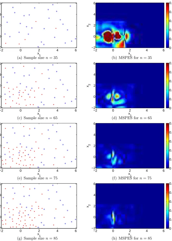
Figure 1: Left column represents the exponential data after 35 (top), 65 (second row), 75 (third row) and 85 (bottom) adaptively chosen samples. In the right column, mean squared prediction error surface (MSPES) is plotted for the corresponding sample size in the same row.
Table 1: f1 and f2 Mean Square Prediction Error for different methods and sample sizes Sample size Method Function n= 35 n= 45 n= 55 n= 65 n= 75 n= 85 ALC with BTMGP f1 0.0131 0.0089 0.0042 0.0026 0.0013 0.0009 f2 0.0159 0.0105 0.0069 0.0043 0.0024 0.0018 ALC with BTGP f1 0.0141 0.0085 0.0048 0.0024 0.0012 0.0009 f2 0.0230 0.0137 0.0096 0.0074 0.0043 0.0029 LHS with BTMGP f1 0.0146 0.0100 0.0092 0.0084 0.0051 0.0032 f2 0.0187 0.0143 0.0129 0.0098 0.0074 0.0051 ALC with MGP f1 0.0448 0.0221 0.0204 0.0098 0.0235 0.0154 f2 0.1870 0.1387 0.1170 0.1364 0.1309 0.1304
We start with an initial set of 30 LHSs (blue circles), and new candidates are chosen from a sequential ALC with BTMGP adaptive sampling as previously described (red stars). The first column of Figure 1 illustrates the sequential adaptive sampling for different sample sizes. Figure 1 shows four different snapshots taken after 5,35,45, and 55 ALC with BTMGP adaptive samples. The ALC with BTMGP prefers samples from the first quadrant, where variations off1
andf2 are high, and results in higher frequency of adaptive sampling in the region, e.g., the left
bottom row plot of the figure has more than 58% of the total samples located in this quadrant. The second row of the figure shows the mean square prediction error surface (MSPES), which corresponds to the sample in the first column. The MSPES is computed as the mean square error of the true value in comparison with the mean of the Bayesian predictive density function as it is described in Section 3.3, for both outputs at particular locations. As we increase the sample size, the MSPES reduces. To better visualize the response surface, we also plot the mean of the Bayesian predictive density function for sample size 85 in Figure 2. Both response surfaces demonstrate very good approximation of the predicted values with the true functions.
x1 x2 prediction of y1 −2 0 2 4 6 −2 −1 0 1 2 3 4 5 6 −0.4 −0.3 −0.2 −0.1 0 0.1 0.2 0.3 0.4 (a) x1 x2 prediction of y2 −2 0 2 4 6 −2 −1 0 1 2 3 4 5 6 0 0.1 0.2 0.3 0.4 0.5 (b)
Figure 2: Average prediction values of the Bayesian treed multivariate Gaussian process.
it to some potential alternatives. For comparison, we use the mean square prediction error (MSPE) integrated over the whole input space. We compare the proposed ALC with BTMGP and the ALC with multiple and independent BTGP described in Gramacy and Lee (2009). This comparison illustrates the importance of modeling the dependence of the output in our multivariate analysis. We also compare the proposed method with the multivariate GP described in Conti and O’Hagan (2010) and sequentially sample the input space using the ALC as described in this paper. This comparison shows the importance of the proposed BTMGP juxtaposed with the MGP model. Moreover, to depict the usefulness of ALC with BTMGP adaptive sampling, we also compare its prediction performance to that of BTMGP when samples are chosen by LHS.
Table 1 shows the MSPE of the four different methods and two output variables (f1,f2) for
different sample sizes. Overall, the MSPE of ALC with BTMGP is smaller than ALC with MGP and LHS with BTMGP. The MSPE of ALC with multiple and independent BTGPs is similar to the MSPE of ALC with BTMGP for the first function (f1). However, in the second function (f2),
the MSPE of ALC with multiple and independent BTGPs is larger than the proposed ALC with BTMGP. For example, when the sample size is 85, ALC with BTMGP produces predictions withM SP E = 0.0009 for f1 and M SP E= 0.0017 for f2. For the same sample size, the mean
square error using ALC with BTGP is M SP E = 0.0009 for f1 and M SP E = 0.0029 for f2.
From these differences, it is evident why the proposed method should be preferred over BTGP (Gramacy and Lee, 2008, 2009) when the outputs are correlated. For the same sample size, the mean square error using LHS with BTMGP isM SP E= 0.0032 forf1 andM SP E= 0.0051 for
f2. A prediction using only a single global multivariate GP for the whole input region affords
an even poorer result. Specifically, M SP E = 0.0154 for f1, and M SP E = 0.1304 for f2. The
stationary assumption is violated. As such, the MGP fails to fit the data. This also is evident by the fact that even when we increase the sample size, there is not much improvement in the MSPE. More sophisticated covariance functions, such as the linear model of coregionalization (LMC) (Banerjee et al., 2004), can be used to improve predictability. However, this is beyond the scope of the present work.
One more interesting observation, shown in Table 1, is decreasing rate of MSPE as we increase the sample size. Using ALC with BTMGP has the fastest MSPE decrease rate as the sample size increases. The ALC with MGP results appear problematic as its MSPE seems to increase the sample size. Even in cases using ALC sampling, a good model should be used for the data to ensure viable results. The combination of the BTMGP model and ALC sampling achieves the best results in terms of prediction performance.
offers an automatic and reliable way for predicting and sampling the input space within the most informative input variables. Moreover, as shown in the online supplementary material, it allows us to focus the sampling into input areas that are more interesting to domain scientists.
6
Application: regenerator of a carbon capture unit
6.1 Carbon capture regenerator unit
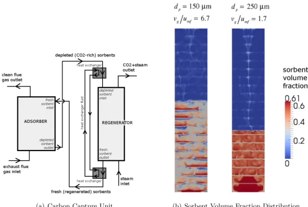
A typical carbon capture unit consists of two devices: the adsorber and the regenerator (Figure 3(a)). Solid sorbent particles capable of reversibly reacting with carbon dioxide (CO2)
is looped through the two devices. In the adsorber, fresh sorbent particles react and trap the CO2 from the exhaust flue gas. The depleted sorbent is then transferred to the regenerator,
where the reverse chemical reaction releases the carbon dioxide back into the gaseous phase for further liquefaction and sequestration (i.e., long-term storage in deep underground reservoirs). The regenerated sorbent particles are recycled back to the adsorber.
In this study, we focus on the regenerator of the capture unit. The bulk of the energy penalty is associated with the regenerator (MacDowell et al., 2010; G´asp´ar and Cormo¸s, 2011) and therefore efforts to increase capture plant efficiency should begin with optimizing the regenerator performance. Details regarding the design and flow in the regenerator are presented in Sarkar et al. (2014). Sorbent flow inside the device is chaotic, and different regions can have varying distribution of sorbent densities (representative snapshots shown in Figure 3(b)). Variations in the local distribution of sorbents, in turn, affects carbon capture rates and device efficiency. Flow of sorbent particles in the regenerator, characterized using the density distribution of sorbent volume fraction, is sensitive to operating conditions such as the velocity of exhaust gases entering the device and the size of sorbent particles, and can sometimes change abruptly with these operating parameters (Sarkar et al., 2014). Therefore, we expect the sorbent volume fraction distribution to be non-stationary with respect to the operating conditions for the regenerator. In this work, though our BTMGP model, we will show that the output (solid fraction distribution) is indeed non-stationary with respect to the input parameters (operating conditions).
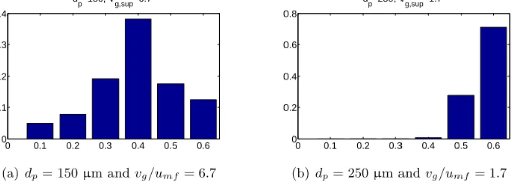
Figure 4 presents the (heterogeneous) distribution functions of the sorbent volume fraction for the two operating conditions shown in Figure 3(b). In this study, we investigate the depen-dence of sorbent distribution function for two input operating conditions: the particle diameter
dp (expressed in micro metres, µm), and the scaled velocityvg/umf of gas injected at the
bot-tom inlet (dimensionless, scaled by a characteristic velocity scale umf; see Gidaspow (1994)). At this point, with little information regarding reaction kinetics, we expect that intermediate solid volume fractions (0.2-0.4) are likely to result in better regenerator performance.
(a) Carbon Capture Unit (b) Sorbent Volume Fraction Distribution
Figure 3: (a) Schematic of a carbon capture unit with adsorber and regenerator. (b) Snapshots of the sorbent volume fraction distribution in the regenerator for two operating conditions: for different sorbent particle diameters (dp) and scaled gas inlet velocities (vg/umf). Blue signifies
empty regions with no particles, while and red represents regions with densely packed sorbents.
computationally expensive CFD simulations may be performed. Approximately 4−7 days of wall-time was required to complete each simulation, running in parallel on 20 processors. The high cost of these CFD models motivates us to develop a BTMGP-based surrogate model capable of predicting the solid fraction distribution in the regenerator which can be used in a sequential sampling design.
6.2 BTMGP on the regenerator of a carbon capture unit
In this section, we focus on the analysis of the sorbent distribution function in a carbon capture unit regenerator (as described in Section 6.1). We begin our analysis with the 36 avail-able simulations of the regenerator reported in Sarkar et al. (2014). Simulations are performed for varying particle diameter dp and scaled gas velocity vg/umf. For our purposes, six bins
are considered sufficient to characterize the distribution function of the solid volume fraction. The full solid fraction range of 0.0 to 0.6 is subdivided into six bins of fixed length, given by [0,0.1],(0.1,0.2],(0.2,0.3],(0.3,0.4],(0.4,0.5],and (0.5,0.6]. As explained in Section 6.1, the frequency distribution function is a key multivariate response that affects the reaction kinetics.
0 0.1 0.2 0.3 0.4 0.5 0.6 0 0.1 0.2 0.3 0.4 dp=150, Vg,sup=6.7 (a)dp= 150µm andvg/umf= 6.7 0 0.1 0.2 0.3 0.4 0.5 0.6 0 0.2 0.4 0.6 0.8 dp=250, Vg,sup=1.7 (b) dp= 250µm andvg/umf= 1.7
Figure 4: Solid fraction distribution function for the two operating cases shown in Figure 3(b).
For each of the 36 simulations, we compute the frequency distribution of the solid fraction as depicted in Figure 4. The height of theith bin represents the relative frequencyπi(x) of the corresponding solid fraction range, where i = 1, . . . ,6 and x = (dp, vg/umf). In order to use
the BTMGP model developed in Section 3, we transform the values of the relative frequency
πi(x) from [0,1] to (−∞,+∞). The logit (logarithm of the odds) transformation, a well-known and popular transformation with the desired properties, is used to transform πi(x), given by
fi(x) = ln (πi(x)/(1−πi(x))), wherei(= 1, . . . ,6) represents theithbin,πi(x) is the probability
value of theithbin, andxrepresents the input variables. We can now build a BTMGP surrogate model for the vector of the logitsf(x) = (f1(x), . . . , f6(x))T. Conditionally on a tree leaf, we
assume thatf(·) follows a multivariate normal distributed (as in Section 2.1) equation 1 with constant mean.
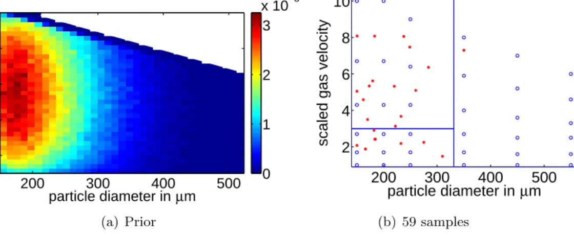
Based on the knowledge gained from a preliminary analysis on the 36 initial simulations (Sarkar et al., 2014), we focus our attention on the region with particle sizedp∈[150µm,270µm] and scaled superficial gas velocity vg/umf ∈ (1.5,9.0). Hence, we generate an artificial two-dimensional Beta distribution that assigns greater importance to this region of interest. Specif-ically, we assume two independent truncated (modified) Beta distributions in the rectangular region, given by [150,550]×[1.0,10.0], and exclude the upper-right corner as the operating conditions lying in that region are not of interest. Figure 5(a) depicts our assumed prior input distribution.
We begin our analysis by running a number of MCMC iterations using the 36 simulations from Sarkar et al. (2014) as the first sample. The hierarchical Bayesian model for the multivariate treed GP in the examples is defined as it is in Section 3. The parameters in the prior distribution of the tree are set α = 0.6 and β = 2 as in Chipman et al. (1998). The mean in each external leaf (subregion) of the BTMGP is modeled as constant. After a number of MCMC iterations, we run the ALC five times while including results from 5 new simulations each time similar to Gramacy and Lee (2009) and the artificial example setting. The inputsdp andvg/umf for these
particle diameter in µm
scaled gas velocity
200 300 400 500 2 4 6 8 0 1 2 3 x 10⁻³ (a) Prior 200 300 400 500 2 4 6 8 10
scaled gas velocity
particle diameter in µm
(b) 59 samples
Figure 5: (a) Prior input probability and (b) 23 ALC with BTMGP samples and the maximum a posteriori (MAP) estimation of the Bayesian tree. The existing input samples are denoted with blue circles and the sequential ALC within BTMGP samples with red stars.
5 additional simulations are chosen based on the BTMGP uncertainty coupled with the input prior distribution. Hence, in addition to the initial set of 36 simulations, 25 more simulations are performed during the five ALC runs ofStep 5.
Along with the prior input distribution, Figure 5 shows the initial observations (blue circles), the sequential adaptive samples (red stars), and the MAP estimation of the Bayesian tree. However, 2 of the 25 additional simulations performed using Multiphase Flow with Interphase eXchanges (MFIX) failed to converge satisfactorily. Instead of 25 sequential adaptive samples, only 23 samples are included in Figure 5(b). To better understand the BTMGP in this problem, we also present the MAP estimation of the Bayesian tree calculated with 59 observations and 30000 MCMC iterations in Figure 5(b), reviling are three distinct subregions as the maximum a posteriorly (MAP) of the Bayesian tree. Scaled gas velocity between 1.5 and 4.0 appears to have 10 ALC with BTMGP samples, and it is an area where non-stationarity is observed. In contrast, for scaled gas velocity between 7.0 and 10.0, the model appears to be quite smooth, and only 4 ALC with BTMGP samples are selected.
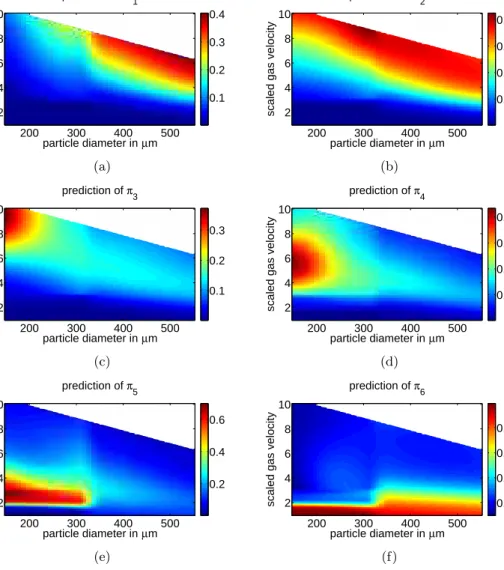
Figure 6 shows the prediction surface of the six different probabilities πi using BMA in a dense grid (70×70). As mentioned previously, operating conditions lying in the upper-right corner are not of interest. Therefore, no simulations are performed for those values. If good regeneration is expected for an intermediate solid fraction range of, say, 0.3 to 0.4, the areas of interest would be regions where π4 is large. From Figure 6(d), the region where π4 is large is
given by dp ∈(150µm,250µm) and scaled gas velocity vg/umf ∈(4.0,8.0). As mentioned, we
pay particularly close attention to this region. Other probabilities may also be of interest. For example, we may want to avoid the regions whereπ1 andπ6 are large, regions with very low or
particle diameter in µm
scaled gas velocity
prediction of π 1 200 300 400 500 2 4 6 8 10 0.1 0.2 0.3 0.4 (a) particle diameter in µm
scaled gas velocity
prediction of π 2 200 300 400 500 2 4 6 8 10 0.05 0.1 0.15 0.2 (b) particle diameter in µm
scaled gas velocity
prediction of π 3 200 300 400 500 2 4 6 8 10 0.1 0.2 0.3 (c) particle diameter in µm
scaled gas velocity
prediction of π 4 200 300 400 500 2 4 6 8 10 0.1 0.2 0.3 0.4 (d) particle diameter in µm
scaled gas velocity
prediction of π 5 200 300 400 500 2 4 6 8 10 0.2 0.4 0.6 (e) particle diameter in µm
scaled gas velocity
prediction of π 6 200 300 400 500 2 4 6 8 10 0.2 0.4 0.6 0.8 (f)
Figure 6: BMA prediction surface of the six different probabilities, as defined above, for different particle diameters in µmand scaled gas velocities.
very high solid fractions.
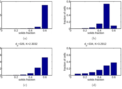
To better evaluate the different models’ prediction abilities, a cross-validation analysis is conducted. We sample the computer code four more times for different combinations of particle diameterdp and scaled gas velocityvg/umf. Figure 7 shows the six bin empirical solid fraction
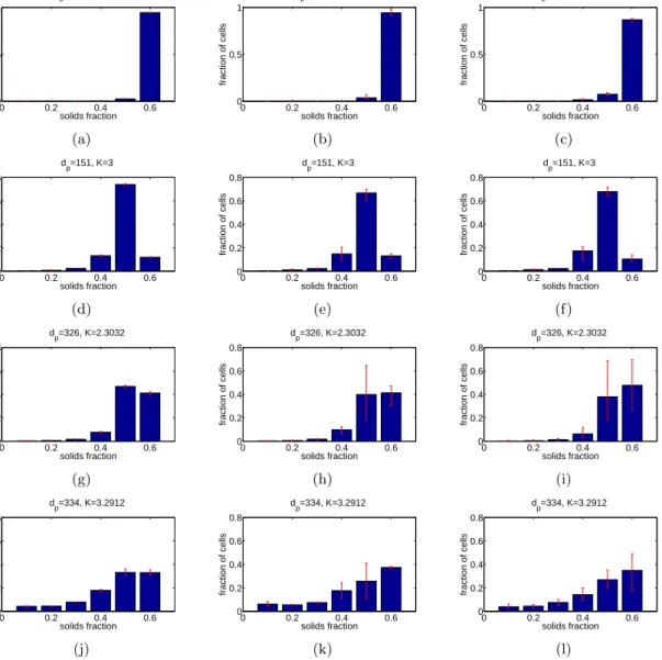
distribution for these four different combinations. We compute and compare the predicted solid fraction distribution of four input values using the multivariate GP with separable function, the BTGP (Gramacy and Lee, 2008), and the proposed BTMGP. Figure 8 illustrate the empirical and prediction probabilities with a 95% prediction interval using the MGP with separable func-tion (first column), the BTGP proposed by Gramacy and Lee (2008) (second column), and the proposed BTMGP (third column).
0 0.2 0.4 0.6 0 0.5 1 solids fraction fraction of cells d p=154, K=1.36 (a) 0 0.2 0.4 0.6 0 0.2 0.4 0.6 0.8 solids fraction fraction of cells d p=151, K=3 (b) 0 0.2 0.4 0.6 0 0.2 0.4 0.6 0.8 solids fraction fraction of cells d p=326, K=2.3032 (c) 0 0.2 0.4 0.6 0 0.2 0.4 0.6 0.8 solids fraction fraction of cells d p=334, K=3.2912 (d)
Figure 7: Real computer code results for four different combinations of particle diameterdp and
scaled gas velocityvg/umf.
Compared with MGP, BTMGP performs better. The mean of the predictions also is closer to the real computer experiment simulation. Specifically, the MSPE using BTMGP is 0.0097, and the MSPE using MGP is 0.0216. However, predictions based on the BTMGP have larger variability due to independent assumption in the subregions associated with the Bayesian tree. Confidence intervals based on the proposed BTMGP are larger than those based on MGP. This variation can be reduced by employing Bayesian tree techniques used in Konomi et al. (2013), which defines dependent covariance functions for each subregion. However, this is beyond the scope of this paper.
In comparison with the BTGP, BTMGP performs also better. The MSPE using multiple BTGP is 0.0119, which is significantly higher than the MSPE using BTMGP. One interesting observation for the predicted solid fraction distribution with BTGP is that for the same input it has different prediction interval (PI) lengths for the six predicted bars. This is due to the fact that BTGP uses independently six simple Bayesian trees which may be different to each other. For some of the predicted bars the 95% PI lengths are similar to the BTMGP intervals. Meanwhile, for others, they are different. For example, the PI of the fifth predicted bar (π5) of
the solid fraction distribution using BTGP for input locations (326,2.3032) and (334,3.2912) have similar PI lengths to the corresponding PI lengths using BTMGP, while the sixth prediction bar (π6) have smaller PI lengths. However, the accuracy is not necessary better. On the contrary,
0 0.2 0.4 0.6 0 0.5 1 solids fraction fraction of cells d p=154, K=1.36 (a) 0 0.2 0.4 0.6 0 0.5 1 solids fraction fraction of cells d p=154, K=1.36 (b) 0 0.2 0.4 0.6 0 0.5 1 solids fraction fraction of cells d p=154, K=1.36 (c) 0 0.2 0.4 0.6 0 0.2 0.4 0.6 0.8 solids fraction fraction of cells dp=151, K=3 (d) 0 0.2 0.4 0.6 0 0.2 0.4 0.6 0.8 solids fraction fraction of cells dp=151, K=3 (e) 0 0.2 0.4 0.6 0 0.2 0.4 0.6 0.8 solids fraction fraction of cells dp=151, K=3 (f) 0 0.2 0.4 0.6 0 0.2 0.4 0.6 0.8 solids fraction fraction of cells dp=326, K=2.3032 (g) 0 0.2 0.4 0.6 0 0.2 0.4 0.6 0.8 solids fraction fraction of cells dp=326, K=2.3032 (h) 0 0.2 0.4 0.6 0 0.2 0.4 0.6 0.8 solids fraction fraction of cells dp=326, K=2.3032 (i) 0 0.2 0.4 0.6 0 0.2 0.4 0.6 0.8 solids fraction fraction of cells d p=334, K=3.2912 (j) 0 0.2 0.4 0.6 0 0.2 0.4 0.6 0.8 solids fraction fraction of cells d p=334, K=3.2912 (k) 0 0.2 0.4 0.6 0 0.2 0.4 0.6 0.8 solids fraction fraction of cells d p=334, K=3.2912 (l)
Figure 8: Prediction probabilities and their 95% prediction intervals using different models for four combinations of particle diameterdp and scaled gas velocity vg/umf. The first column
shows the prediction probabilities and their 95% prediction intervals using multivariate GP with separable covariance function. The second column gives the prediction probabilities and their 95% prediction intervals using BTGP, and the third column provides the prediction probabilities and their 95% prediction intervals using the proposed BTMGP.
in most of the cases the mean of BTGP is misspecified, with the most remarcable difference noticed in the input (326,2.3032). The probabilities in this applicatrion are correlated, as such the BTMGP is a better model than BTGP, which assumes independent multivaraite output.
In general, we observe that prediction probabilities for input values close to available obser-vations are more accurate than prediction for input values further away from the obserobser-vations. In particular, prediction probabilities for dp = 151 µm and vg/umf = 3 are more accurate
than prediction probabilities fordp = 334 µm and vg/umf = 3.2912. We also observe that the
probability predictionsπi (histogram bar heights) with values close to 0.5 tend to have larger
uncertainty in comparison toπi values close to 0 and 1. This is expected because the variance
of the proportion is higher when the estimated proportion is close to 0.5.
7
Concluding remarks and extensions
Herein, we developed a Bayesian treed multivariate Gaussian process (BTMGP) that com-bines the Bayesian tree (Chipman et al., 1998; Gramacy and Lee, 2008) and the MGP with a separable covariance function (Mardia and Goodall, 1993; Conti and O’Hagan, 2010). The proposed BTMGP provides a multi-output emulator that can handle problems with discontinu-ities and localized features. The form of the separable covariance function simplifies the form of the inverse and determinant of the covariance matrix involved and, therefore, facilitates the computations within MCMC updates. Moreover, the prior specification of the MGP parameters leads to efficient local proposals in theGrow and Prune operations of the Bayesian tree. Only the parameters of the correlation function need to be updated at each MCMC iteration for prediction purposes. Moreover, we introduce numerical stability in the covariance function by adding a nugget term without increasing the computational complexity of the model.
We also propose a sequential experimental design technique based on the BTMGP predictive uncertainty. We extend the univariate ALC to properly deal with multivariate output and incorporate knowledge gained from prior studies. The proposed ALC with BTMGP adaptive sampling offers an automatic and reliable way to sample the input space and perform prediction at a low computational cost. As shown in this paper, the proposed method performs better than the multiple BTGP when the output variables are dependent.
The separable covariance function used in the proposed BTMGP can be extended into more general models such as the Linear model of Coregionalization (LMC) (Banerjee et al., 2004). Moreover, the proposed model can be extended to multiple Bayesian trees such that each output has its own Bayesian tree structure. The proposed model performs acceptably well when the output variables are dependent but one could expect a potential problematic behavior in the independent scenario. The LMC covariance function is more general than the separable covariance function and may result in better fitting. Moreover, multiple Bayesian tree may be more appropriate for some applications when some of the outputs are independent. Despite the nice features of these extensions, they involve more parameters and they are expected be computationally more expensive. A more comprehensive study of the selection of multivariate covariance functions and the use of multiple Bayesian trees is left for future research.
regen-erator of carbon capture system. We define the problem and transform the data to a form such that we can apply the proposed model. In our numerical example, we begin with 36 samples collected from a previous study and sequentially generate 23 more samples using ALC with BTMGP. Then, we produce predictions of the solid fraction distribution in the regenerator for different combinations of bottom inlet gas flow rate (gas velocity) and sorbent size (particle diameter). We envision that the model and computationally efficient method developed in this paper have the potential to analyze similar computer experiments. Moreover, the BTMGP can be used as a computationally efficient model to deal with high-dimension non-stationary spatial data sets with multivariate output.
Acknowledgments The research at Pacific Northwest National Laboratory (PNNL) was supported by the Department of Energy Carbon Capture Simulation Initiative. PNNL is oper-ated by Battelle for the U.S. Department of Energy under Contract DE-AC05-76RL01830. We thank the referees and the editors for their valuable comments.
References
Banerjee, S., Carlin, B., and Gelfand, A. (2004),Hierarchical Modeling and Analysis for Spatial Data, Boca Raton, FL: Chapman & Hall-CRC.
Berger, J. O., Oliveira, V. D., and Sanso, B. (2001), “Objective Bayesian Analysis of Spatially Correlated Data,”Journal of the American Statistical Association, 96, 1361–1374.
Bilionis, I., Zabaras, N., Konomi, B., and Lin, G. (2013), “Multi-output separable Gaussian process: Towards an efficient, fully Bayesian paradigm for uncertainty quantification,”Journal of Computational Physics, 241, 212–239.
Chipman, H., George, E., and McCulloch, R. (1998), “Bayesian CART Model Search,”Journal of the American Statistical Association, 93, 935–960.
Cohn, D. A. (1996), “Neural Network Exploration Using Optimal Experiment Design,”Advances in Neural Information Processing System, 6, 679–686.
Conti, S. and O’Hagan, A. (2010), “Bayesian emulation of complex multi-output and dynamic computer models,” Journal of Statistical Planning and Inference, 140, 640–651.
Cressie, N. (1993), Statistics for Spatial Data. 2nd edition, New York: John Wiley and Sons Inc.
Denison, D., Mallick, B., and Smith, A. (1998), “A Bayesian CART Algorithm,” Biometrika, 85, 363–377.
G´asp´ar, J. and Cormo¸s, A. (2011), “Dynamic modeling and validation of absorber and desorber columns for post-combustion CO2 capture,” Computers & Chemical Engineering, 35, 2044–
2052.
Gelfand, A. E. and Smith, A. F. M. (1990), “Sampling-Based Approaches to Calculating Marginal Densities,”Journal of the American Statistical Association, 85, 398–409.
Gidaspow, D. (1994), Multiphase Flow and Fluidization: Continuum and Kinetic Theory De-scriptions, Academic Press, San Diego, 1st ed.
Giles, M. B. (2008), “Multi-level Monte Carlo path simulation,” OPERATIONS RESEARCH, 56, 607–617.
Godsill, S. (2001), “On the relationship between Markov chain Monte Carlo methods for model uncertainty,”Journal of Computational and Graphical Statistics, 10, 230–248.
Gramacy, R. B. and Lee, H. K. H. (2008), “Bayesian treed Gaussian process Models with an application to computer modeling,” Journal of the American Statistical Association, 103, 1119–1130.
— (2009), “Adaptive Design and Analysis of Supercomputer Experiments,”Technometrics, 51, 130–145.
Green, P. (1995), “Reversible Jump Markov Chain Monte Carlo Computation and Bayesian Model Determination,” Biometrika, 82, 711–732.
Hastings, W. K. (1970), “Monte Carlo sampling methods using Markov chains and their appli-cations,”Biometrika, 57, 97–109.
Hjort, N. and Omre, H. (1994), “Topics in Spatial Statistics [with Discussion, Comments and Rejoinder],” Scandinavian Journal of Statistics, 289–357.
Iman, R. L. and Conover, W. J. (1980), “Small sample sensitivity analysis techniques for com-puter models, with an application to risk assessment,”Communications in Statistics - Theory and Methods, 9.
Karagiannis, G. and Andrieu, C. (2013), “Annealed Importance Sampling Reversible Jump MCMC Algorithms,” Journal of Computational and Graphical Statistics, 22, 623–648.
Kim, H.-M., Mallick, B., and Holmes, C. (2005), “Analyzing nonstationary spatial data using a piecewise Gaussian process,”Journal of the American Statistical Association, 470, 653–658.
Konomi, B., Sang, H., and Mallick, B. (2013), “Adaptive Bayesian nonstationary modeling for large spatial datasets using covariance approximations,” Journal of Computational and Graphical Statistics, doi: 10.1080/10618600.2013.812872.
Liu, J., Wong, W., and Kong, A. (1994), “Covariance structure of the Gibbs sampler with applications to the comparisons of estimators and augmentation schemes,” Biometrika, 81, 27–40.
MacDowell, N., Florin, N., Buchard, A., Hallett, J., Galindo, A., Jackson, G., Adjiman, C., Williams, C., Shah, N., and Fennell, P. (2010), “An overview of CO2 capture technologies,”
Energy & Environmental Science, 3, 1645–1669.
Mardia, K. V. and Goodall, C. R. (1993), “Spatial temporal analysis of multivariate environ-mental monitoring data,” In Multivariate Environmental Statistics (G. P. Patil and C. R. Rao, eds.), 347–386.
Mueller, P. (1993), “Alternatives to the Gibbs sampling scheme,” Tech. rep., Institute Statistics and Decision Sciences, Duke University.
Sarkar, A., Pan, W., Suh, D., Huckaby, E., and Sun, X. (2014), “Multiphase flow simulations of a moving fluidized bed regenerator in a carbon capture unit,” Powder Technology, In press.
Seo, S., Wallat, M., Graepel, T., and Obermayer, K. (2000), “Gaussian Process Regression: Active Data Selection and Test Point Rejection.” IEEE. In Proceedings of the International Joint Conference on Neural Networks, III, 241–246.
Disclaimer: This journal article was prepared as an account of work spon-sored by an agency of the United States Government. Neither the United States Government nor any agency thereof, nor any of their employees, makes any war-ranty, express or implied, or assumes any legal liability or responsibility for the accuracy, completeness, or usefulness of any information, apparatus, product, or process disclosed, or represents that its use would not infringe privately owned rights. Reference herein to any specific commercial product, process, or service by trade name, trademark, manufacturer, or otherwise does not necessarily consti-tute or imply its endorsement, recommendation, or favoring by the United States Government or any agency thereof. The views and opinions of authors expressed herein do not necessarily state or reflect those of the United States Government or any agency thereof.