Union College
Union | Digital Works
Honors Theses Student Work
6-2014
Does Public School Administrative Spending
Affect District House Prices?
Catherine Degen
Union College - Schenectady, NY
Follow this and additional works at:https://digitalworks.union.edu/theses
Part of theEducational Administration and Supervision Commons, and theEducation Economics Commons
This Open Access is brought to you for free and open access by the Student Work at Union | Digital Works. It has been accepted for inclusion in Honors Theses by an authorized administrator of Union | Digital Works. For more information, please [email protected].
Recommended Citation
Degen, Catherine, "Does Public School Administrative Spending Affect District House Prices?" (2014).Honors Theses. 510. https://digitalworks.union.edu/theses/510
Does Public School Administrative Spending Affect District House Prices?
by
Catherine A. Degen
* * * * * * * * *
Submitted in partial fulfillment of the requirements for
Honors in the Department of Economics
UNION COLLEGE June, 2014
ii
ABSTRACT
DEGEN, CATHERINE A. Does Public School Administrative Spending Affect District House Prices? Department of Economics, June 2014.
ADVISOR: Stephen J. Schmidt
Public schools are often criticized for the way in which they elect to distribute their limited resources. Perhaps the most critical assets for schools are teachers and
administrators, and the compensation of these individuals varies widely amongst public school districts. There exists an optimal level of spending on district administration. Districts that pay administrators above or below this optimal point are likely not allocating their resources in the best possible manner, and educational quality may suffer. We
hypothesize that within districts where either of the above situations is the case, home prices will be lower, as homebuyers will be less willing to pay for homes within a district where the schools do not function efficiently and allot taxpayer dollars well. Using boundary discontinuity methods, we find a district's amount of administrative spending per pupil, to be highly significant and inversely related to district house prices. We also find a significant inverse relation between a district's level of non-administrative spending per pupil and home values, and a significant positive correlation between a district's level of wealth and house prices. Thus, based upon its valuation by homebuyers, we conclude that school spending within Capital District schools is currently above its optimum point. Additionally, we find the significance of district size, student-to teacher ratio and test scores, to district house prices, to vary by specification, and do not find race or teacher salaries to be significant.
iii
TABLE OF CONTENTS
Table of Figures v
Chapter One: Introduction 1
Chapter Two: A Review of School Costs and Housing Prices 5
A. School Spending and Student Performance 5
A.1. Overall Levels of School Spending and Student Performance 5 A.2. Levels of Administrative School Spending and Student 9
Performance
B. Public School Quality and House Prices 13
B.1. Capitalization of School Test Scores in House Prices 13 B.2. Capitalization of Other Distinct Measures of Student 18
Performance in House Prices
B.3. Capitalization of Value-added Measures in House Prices 20 B.4. Capitalization of Per Pupil Expenditures in House Prices 23 B.5. Capitalization of Racial Composition in House Prices 25 B.6. Capitalization of Other Variables in House Prices 27 Chapter Three: Model and Theory
A. The Hedonic Housing Price Model 28
B. The Explanatory Variables 31
B.1. House Characteristics 31
B.2.The Regressor of Primary Interest: Administrative 32 Expenditures
B.3. Other Independent Variables 34
B.4. Border Dummies 38
Chapter Four: Data 40
A. District Borders 40
B. School District Data 43
C. House Selection 44
D. House Data 45
Chapter Five: Statistical Tests of Theory 47
A. Regression Equations 47
B. Significance of Results 49
B.1. Home Characteristics 49
B.2. Administrative Spending Levels 50
B.3. Other District Characteristics 52
B.4. The Border Dummies 57
iv
Chapter Six: Policy Implications 59
A. Public School Administrative Spending in the United States 59 B. Public School Administrative Spending in New York State 61
C. Potential Remedies 62
Chapter Seven: Suggestions and Conclusions 65
A. Suggestions for Future Studies 65
B. Conclusions 66
Bibliography 68
v
TABLE OF FIGURES
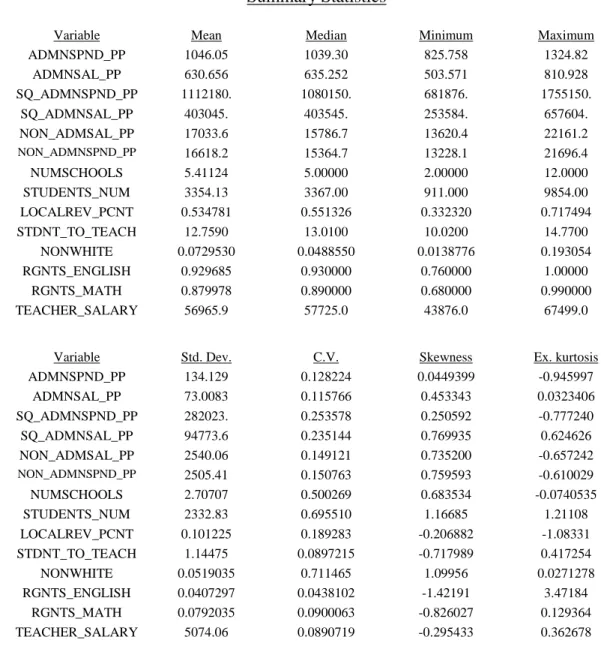
Figure 1: Map of Capital Region School Districts 73 Figure 2: Summary Statistics: School District Level 74 Figure 3: Summary Statistics: Home Characteristics 75
Figure 4: Border Dummy Descriptions 76
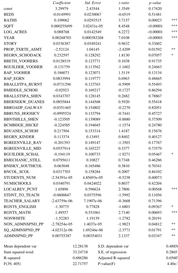
Figure 5: Primary OLS Regression: Dependent Variable is Log of House 77 Price (LOG_SALE_PRICE) and Administrative Spending
Variable is Total Administrative Spending per Pupil (ADMNSPND_PP)
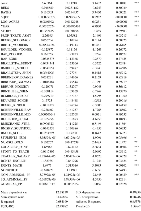
Figure 6: Secondary OLS Regression: Dependent Variable is Log of 78 House Price (LOG_SALE_PRICE) and Administrative Spending Variable is Total Administrative Salary Spending per Pupil (ADMNSAL_PP)
1
CHAPTER ONE
Introduction
Public schools are often criticized for the way in which they elect to distribute their limited resources. Perhaps the most critical assets for schools are teachers and
administrators, and the compensation of these individuals varies widely amongst public school districts. There exists an optimal level of pay for district administrators. Districts that pay administrators above or below this optimal point are likely not allocating their resources in the best possible manner, and educational quality may suffer.
Resources lost to excess administration are resources that districts could have allocated to other things that would improve students' educational experiences (e.g. more advanced placement courses, music programs, and physical education). Conversely, districts that do not adequately compensate their administrators may struggle to attract quality personnel, potentially causing a decline in educational quality. School districts need a strong administration that is capable of overseeing school programs and resolving issues when they arise. Thus, we take the level of administrative spending in a district to be symbolic of the district's ability to allocate its resources efficiently.
We hypothesize that within districts where either of the above situations is the case, home prices will be lower, as homebuyers will not want to live in a district whose schools do not function efficiently and allot taxpayer dollars well. By inefficiently
allocating their resources, schools are likely hurting the quality of the education they offer their students. Parents and other taxpayers will notice that these schools are not allocating their resources well, and will be less willing to pay less for homes within these districts, and thus house prices there will fall. We hypothesize the relationship between house
2
prices and administrative spending to be ∩-shaped, with the optimal point of administrative spending being the maximum of the curve.
The economic literature has clearly demonstrated that there is a relationship between public school quality and district house prices. This literature has shown a strong positive correlation between test scores in school districts and the house prices within those districts (Brasington 1999, Downes and Zabel 2002, Crone 2006, etc.). The literature has shown that correlations between other quality measures (e.g. per student spending, value-added, class size) and house prices are weaker (Brasington and Haurin 2006, Seo and Simons 2009, Iberman and Lovenhiem 2013, etc.). We anticipate both administrative salary spending and total administrative spending per pupil, measures of school efficiency, to be capitalized in house prices as well. Previous economic studies have observed the relationship between administrative spending and student performance, but to our
knowledge, no study has investigated the potential correlation of administrative spending levels and house prices (Brewer 1996, Jaggia and Kelly-Hawke 1999, Jacques and Brorsen 2002, etc.).
Independent variables that we will control for within the hedonic model include: house characteristics (number of bedrooms, number of bathrooms, year built, square footage, lot size, stories, property tax rate), non-administrative expenditures per pupil, student test performance, the student-to-teacher ratio, race, poverty, average teacher salaries, and the regressor of primary interest, total administrative spending per pupil. We will observe a sample of 445 houses from New York State's Capital Region that sold in 2012 or 2013. Within our sample, we will only include houses located in the proximity of the district boundary. This use of boundary methods will help us to eliminate much of the
3
omitted variable bias that exists in the equation due to our inability to sufficiently control for all neighborhood characteristics.
Using these boundary discontinuity methods, we find a district's amount of
administrative spending per pupil, to be highly significant and inversely related to district house prices. However, though definitively negative, we do not find the relationship between a district's level of administrative salary spending per pupil, a subset of total administrative spending, and home values to be of significance. We find a significant inverse relation between a district's level of non-administrative spending per pupil and home values, and a significant positive correlation between a district's level of wealth and house prices. Thus, based upon its valuation by homebuyers, we conclude that school spending within Capital District schools is currently above its optimum point.
Additionally, we find the significance of district size, student-to teacher ratio and test scores, to district house prices, to vary by specification, and do not find race or teacher salaries to be significant.
In recent years, New York State, as the nation, has witnessed a substantial increase in its number of public school administrators. From fiscal year 1992 to fiscal year 2009, New York State experienced a 4 percent increase in its number of public school students, but a 26 percent increase in its number of administrators and non-teaching staff (Scafidi 2013). One would expect that increases in administrative expenditures would correlate to increases in student test performance. However, this has not been the case. Both nationally and within New York State, increases in administrative spending have not been shown to correlate with improved school quality and student performance, and thus we conclude that administrative spending levels within the United States are currently above the
4
optimal (Scafidi 2013). Our regression results demonstrate this to be the case within the Capital Region as well.
5
CHAPTER TWO
A Review of School Costs and Housing Prices
To our knowledge, the economic literature has not explored the potential
correlation between levels of administrative spending and district house prices, as we will discuss in this paper. Thus, we are not able to perform a literature review of papers that investigate this specific relationship. As an alternative, we will review the literature on school costs, specifically administrative spending, and house prices each individually.
A. School Spending and Student Performance
To date, the majority of economic literature on school spending pertains to its correlation with student performance. Though economists have discussed the issue extensively in the literature, they have yet to reach a consensus. The literature better defines the correlation between levels of school administrative spending per pupil and student performance, suggesting an inverse relationship between the two.
A.1. Overall Levels of School Spending and Student Performance
Communities are deeply invested in their public schools and many community members have strong feelings about the magnitude of local school budgets. Schools generate positive externalities for their communities and school quality is an important determinant of students' future productivity and earnings. As cited by Hanushek (1996), national school spending totals about four percent of the U.S. gross domestic product, and is the most significant piece of most local government budgets. Thus, the question of whether altering the school budget would influence student performance is of great importance to community members. It is a delicate balance between keeping tax rates low and ensuring that students have the resources they need to succeed.
6
The literature discussion over the connection between school spending and student performance began with a 1966 U.S. Government report on educational equality,
frequently cited as the "Coleman Report." The report found that school expenditures have only a minor impact on student achievement, concluding that family background is instead the most significant determinant of achievement (Coleman et al. 1966). Twenty years later, Hanushek cited similar findings (1986, 1989). Analyzing the then existing body of
literature, Hanushek concluded that school expenditures have no relation to test
performance, once one controls for family background (1986, 1989). Instead of requesting increased funding, Hanushek suggests that schools should instead provide teachers with performance incentives (1989). His findings reflect an important synthesis of the existing research, as his search for data uncovered 187 "qualified studies" in 38 separately published books and articles (1989).1 The data used in these "qualified studies" is representative of all
regions of the Unites States and contains information on multiple grade levels, different measures of performance and different statistical approaches (1989).2
Hedges, Laine and Greenwald (1994) (henceforth HLG) contest Hanushek's (1986, 1989) results, as they instead find a positive correlation between levels of school spending
1 Hanushek (1989) defines a " qualified study" as a "production-function estimate that is: (1) published in a book or refereed journal; (2) relates some objective measure of student output to characteristics of the family and the schools attended; and (3) provides information about the statistical significance of estimated
relationships" (46).
2 "About one-third draw their data from a single school district, whereas the remaining two-thirds compare school performance across multiple districts. Additionally, a majority of the studies (104) use individual students as the unit of analysis, with the remainder relying upon aggregate school, district, or state-level data. The studies are about evenly split between primary schooling (grades 1-6) and secondary schooling (grades 7-12). Over 70 percent of the studies measure school performance by some kind of standardized test. However, those that use non-test measures (such as dropout rates, college continuation, attitudes, or
performance after school) are for obvious reasons concentrated in studies of secondary schooling. There is no indication that differences in sample and study design lead to differences in conclusions, and thus only an overall tabulation of results is presented." (Hanushek 1989, 46)
7
and student performance. Using a meta-analysis method, they conclude that a ten percent increase in a school's real resources will improve students' measured achievement by 0.7 standard deviations (HLG 1994). They claim that Hanushek's (1989) "vote counting methodology" gives no indication of the magnitude of relationships between variables and assert that his tests had a low degree of statistical power (HLG 1994). Hanushek (1994) immediately responds to this criticism, claiming that Hedges, Laine and Greenwald's meta-analysis is flawed, as they omitted many of the studies that show increasing
expenditures has no effect from their analysis. To further back up his initial conclusions, Hanushek (1994) cites a statistic from the U.S. Department of Education: in the 25 years to 1994, real expenditures per pupil rose more than 100 percent, while student
performance remained constant at best and likely declined. Despite this, Hedges and Greenwald (1996) again refute Hanushek's findings. They claim that expansion in the level and comprehensiveness of education and a decline in the social capital available in families have acted as substitutes for school resources, and thus argue that increased resources do in fact result in increased student productivity (1996).
In recent years, Hanushek's findings (1986, 1989, and 1994) have remained fiercely debated, and a number of more recent studies have found at least a weak
correlation between per pupil school expenditures and student achievement. Sander (1999) finds a slightly positive correlation between these two variables. Using 1996 data from the Illinois Goal Assessment Program, standardized tests issued by the state all third and eighth grade students; Sander (1999) concludes that expenditures per pupil have a significant link to students' results on the eighth grade math assessment. Though
8
per pupil would have to more than double to increase test scores by one standard deviation" (Sander 1999, 229).
Papke (2005) also cites a positive correlation between spending per pupil and student achievement, a finding based on data solely from within the state of Michigan. Proposition A, passed by the Michigan State government in 1994, greatly altered the funding structure of the state's public K-12 schools, thus making Michigan an optimal place to perform this study. Though Papke (2005) has access to all Michigan state test scores from 1992 to 1998, she elects to focus specifically on fourth grade math test scores, as this data set is the most complete and consistent. Papke (2005) finds that a ten percent increase in a district's real spending increases school pass rates on the fourth grade state math test by between one and two percentage points. Notably, her findings also show that this statistically significant effect is largest for schools with initially poor performance (Papke 2005).
We must note, however, that these studies by Sander (1999) and Papke (2005) only incorporate data from a single state. In contrast, Hanushek's (1989, 1994, and 1996)
studies utilized a sample with a significantly greater geographic and economic diversity. It is possible that funding may affect schools in different states differently, as the states' educational systems and levels of expenditures vary greatly. For instance, in contrast to the findings of Sander (1999) and Papke (2005), a recent study of Vermont schools by Sherlock (2011) finds no significant correlation between levels of school spending and student test performance. Measuring the impact of changes under Vermont's Equal Education Opportunity Act, Sherlock (2011) concludes that this shift in resources had no significant effect on the passing rates of the state's fourth grade reading and writing tests.
9
She finds a slightly positive, though insignificant, correlation between per student spending and the passing rate on the fourth grade state math test. Sherlock (2011) also provides suggestive, though inconclusive, evidence that resources are more effective at increasing passing rates at initially lower spending schools, though not at lower achieving schools.3
If considering the law of decreasing marginal returns, this suggestion is logical.
A.2. Levels of Administrative School Spending and Student Performance
There is no clear consensus within the economic literature about the relationship between the level of public school spending and the level of student achievement. However, the literature has suggested that there is an inverse correlation between a district's level of administrative inputs (on a per student basis) and student performance within that district. Brewer (1996) was one of the first to extensively investigate this relationship, and argues that test scores and per pupil administrative expenditures are simultaneously related. For this reason, Brewer (1996) elects to use a simultaneous equations estimator to determine the correlation between the variables. His data comes exclusively from New York State, and he examines a panel of school districts over the 1978 to 1987 period. Separating the data into elementary, middle school and high school segments, overall, he finds a weak negative correlation between administrative inputs per student and the pass rates on state tests, with inconsistency between the models used (Brewer 1996).4 Brewer concludes that, "more administration lowers teacher productivity
and has a negative marginal product at current expenditure levels" (1996, 998). Though
3 It is important to note that lower spending schools do not necessarily have low levels of achievement. It is very possible for schools to have below average spending, and for a variety of reasons (e.g. economies of scale), still have high levels of student achievement.
4 Brewer (1996) uses an ordinary least squares model (OLS), a fixed effects model and a three-stage least squares regression mode (3SLS) model within this study.
10
Brewer (1996) finds a weak correlation between per pupil spending and student performance, the significance of his results is weak, potentially indicating that his instruments were inadequate.5
In line with the findings of Brewer (1996), Jaggia and Kelly-Hawke (1999) conclude that there is an inverse relationship between per pupil administrative spending and student test performance. Jaggia and Kelly-Hawke (1999) utilize data from the 1992 Massachusetts Educational Assessment Program (MEAP) test. The State of Massachusetts administers MEAP tests annually to all fourth, eighth and twelfth grade students to measure student learning.6 Using an ordered logit model, as test results were in groups, Jaggia and Kelly-Hawke (1999) find that per pupil administrative spending is inversely correlated to students' MEAP test performance at all grade levels, and the effect is large enough to be significant at the fourth and eighth grade levels. Resources allocated to administration likely come at the expense of resources for instruction. Jaggia and Kelly-Hawke (1999) also find that family background and the stability of community contribute significantly to student performance.
Similarly, Jacques and Brorsen (2002) conclude that there is an inverse
relationship between per pupil spending on student support services (i.e. administration and counseling) and student performance on standardized tests. They elect to use data from the Oklahoma Department of Education, specifically the results of the state's
5
Brewer (1996) instead found that increasing the number of teachers in a district had the greatest impact on test pass rates.
6 The fact that all of the schools were located within the same state helps to remove a great deal of omitted variable bias from the study (Jaggia and Kelly-Hawke 1999).
11
Criterion Referenced Test (CRT) and Norm Referenced Tests (NRT).7 Jacques and Brorsen's (2002) study corrects for the heteroskedasticity created by differences in school district size, helping to give the model greater statistical power. Using a maximum
likelihood distribution, an alternative to ordinary least squares, Jacques and Brorsen (2002) find a statistically insignificant, negative correlation between per pupil spending on school administration and student performance. They conclude that high administrative spending displaces funds that could be utilized in a more productive manner, and suggest that school administrators may take up valuable student instruction time with
announcements and assemblies (Jacques and Brorsen 2002). Yet, it is important to note, that schools with lower test scores and more problems overall may need to hire more administrators and school counselors, and it is possible that "socioeconomic variables may not fully capture the problems that these schools face" (Jacques and Brorsen 2002, 997).8
Mensah, Schoderbek and Sahay (2013) (henceforth MSS) also examine the relationship between levels of school administrative spending and student achievement. They note that in recent years a number of states have passed measures to limit
administrative expenses in their public schools. At the forefront of this movement was the Chicago School Reform Act, passed by the Illinois State Legislature in 1988, which
imposed limits on the maximum levels of non-instructional costs within the Chicago public school system (MSS 2013). New Jersey, the state of origin for MSS's (2013) data, passed
7 The State administers the CRT to students in grades 5, 8 and 11 to determine if students are at grade level. The State also administers the NRT to students in grades 3 and 7 as a test of knowledge, not to ensure the correct grade level. Test results were available by school district and grade for each district in the sample for 1994-1995 (Jacques and Brorsen 2002).
8
This issue may cause omitted variable bias within Jacques and Brorsen's (2002) equations. Specifically, this explains why we expect an ∩-shaped relation between administrative spending levels and house prices, in which the optimal level of administrative spending varies from district to district.
12
legislation in 2004, anchoring per pupil administrative costs to the lower of, "per-pupil admin costs average for the district's region" and "the prior year's admin costs adjusted by the cost of living or 2.5 percent, whichever is less" (MSS 2013, 2). In 2011, New Jersey passed another law limiting the level of public school administrative spending, instituting a salary cap for district superintendents. Under this new cap, the maximum yearly salary a superintendant can be paid is $175,000 per year, for large districts with over 6,500 students, with less for smaller districts (MSS 2013). These laws put New Jersey at a competitive disadvantage in attracting well-qualified administrators and encouraged an exodus of school administrators to other states without pay restrictions (MSS 2013).
Due to these changes in school administrative pay scales, and the variance thus produced, New Jersey is an excellent place to study the effect of administrative
expenditures on test scores. Mensah, Schoderbek and Sahay (2013) use data from the New Jersey Department of Education, specifically a sample of 217 Kindergarten to Grade 12 districts for the years 2002-2009. Their dependent variable is the weighted test score averages for the state's standardized tests, administered at the fourth, seventh and twelfth grade levels. Using a one-way fixed effects model, MSS (2013) find administrative spending per pupil to be negatively associated with student test performance, though this correlation they do not find the correlation to be significant in the two-way models.9
Overall, the literature suggests that there is at least a weak negative correlation between administrative expenditures per pupil and test scores (Brewer 1996, Jaggia and Kelly-Hawke 1999, Jacques and Brorsen 2002, MSS 2013). The relationship between
9 The two way models analyzed were the way fixed effects model (time and school district) and the two-way random effects model. The one-two-way fixed effects model is only fixed time-wise.
13
administrative spending per student and district house prices has yet to be defined within the economic literature.
B. Public School Quality and House Prices
It is clear that the quality of local public schools is capitalized into the housing market, but the question of what is the most appropriate measure of school quality
remains. To date, the literature has shown a reasonably strong positive correlation between district schools' performance on state tests and house prices within that district. The
literature has also explored average district expenditures per student, value-added, and student to teacher ratios as potential measures of school quality, but the correlations of these variables with the housing market are found to be significantly weaker.
B.1. Capitalization of School Test Scores in House Prices
One of the earliest papers to analyze the capitalization of school test scores in district house prices is that of Hayes and Taylor (1996). Using data from the Dallas Independent School District (DISD), they find that district house prices reflect school test scores and that homebuyers value the marginal effects of schools on student performance ("value-added"). The significance of their initial findings, however, is limited, as the study's sample size is quite small. To measure the housing market, Hayes and Taylor (1996) used the selling prices of the 288 DISD properties that sold in July 1987. The breadth of test scores used is also limited, as the only measure incorporated in the study is average sixth grade achievement on the Iowa Test of Basic Skills; a measure of high school performance is not used.
Later studies build on this early work of Hayes and Taylor (1996), increasing both the number of houses and variety of student test scores included in the sample. Similar to
14
Hayes and Taylor (1996), Brasington (1999) finds a positive correlation between student performance on standardized tests and district house prices. Brasington (1999) uses a significantly larger sample of houses, a greater diversity of properties and an increased variety of performance measures.10 He utilizes data from the Ohio Department of
Education on passage rates of the state's standardized tests, administered to students in grades 4, 9 and 12. For housing prices, Brasington (1999) uses 1991 sample data from major metropolitan communities in Ohio, from 128 different communities for a sample size of over 27,000 houses. This is a significantly larger sample than used in previous studies (Hayes and Taylor 1996). Using both a traditional hedonic price estimation model and a hedonic model corrected for spatial autocorrelation, Brasington (1999) finds that the housing market does indeed value proficiency test passage rates, though not the value-added by the school district.
Black (1999) is a frequently cited paper examining the relationship between school test scores and district house prices. She builds greatly on the existing literature in that she is able to better control for neighborhood characteristics, as well as socioeconomic status, within her sample. To do this, Black (1999) looks only at houses situated on school attendance boundaries, thereby the houses in the sample differ only in what school the children attend. This method successfully removes the variation between neighborhoods. Black (1999) uses test score data from the Massachusetts Educational Assessment Program
10 Brasington (1999) includes a large number of variables in his study. He finds that test scores, per pupil expenditures and student-to-teacher ratios have significant effects on district house prices. This finding is logical, as these measures are widely publicized and easily available to homebuyers. Brasington (1999) concludes that teacher salaries and student attendance may also have some impact on house prices, but the relationship is not significant. He finds that school graduation rates, levels of teacher experience and levels of teacher of education are not capitalized in house prices whatsoever.
15
(MEAP), a standardized test given to all Massachusetts students in grades 4, 8 and 12.11
She sums and averages student math and reading performance in three testing periods (1988, 1990, 1992) in attempt to remove any variance that might occur by using test data from only a single year. Black's (1999) sample of recent house transactions is quite large as well, as she uses the prices from all border purchases and sales from 1993 to 1995 in the Middlesex, Essex and Norfolk counties of Massachusetts - all suburbs of Boston.12
Using a hedonic pricing model, Black (1999) finds that for a five percent increase in test scores, approximately a one standard deviation rise; parents are willing to pay 2.1 percent more for a house in that district.13 She suggests that a move "from a school that
scores in the twenty-fifth percentile of the sample to a school in the seventy-fifth percentile of the sample would result in a house price increase of $5,452" (Black 1999, 595). Black (1999) notes that this result is significantly smaller than that found in many previous studies that did not sufficiently control for neighborhood characteristics, and speculates that these studies likely overestimated the effects of test scores.14
Though Downes and Zabel (2002) also find a positive relationship between school test scores and local house prices, the models used to come to this result differ greatly from those used in other studies. Rather than using recent selling prices for individual homes as their models' dependent variable, Downes and Zabel (2002) use data on estimated home
11 Massachusetts administers MEAP tests in five subject areas: reading, science, social studies, mathematics and writing (Black 1999). Black (1999) elects to use only math and reading scores in her study.
12 These are excellent districts to use in her sample as they are fairly small and their populations are reasonably homogeneous. Within these three counties, there are 39 separate school districts (Black 1999). 13
For a house with the sample's mean price of $188,000, this represents exactly $3,948 more (Black 1999). 14 Black (1999) also notes that the preferences of Boston homeowners may be different from homeowners in other parts of the country. This is logical, as the state of Massachusetts as a whole, places great value on education and is known for having high quality schools.
16
values from the American Housing Survey (AHS). AHS does not include data solely from recently sold homes, rather it contains "detailed information on particular homes through time that includes the current owner’s evaluation of the house price, house characteristics, and self-reported information on the house’s current occupants" (Downes and Zabel 2002, 9). As a measure of student performance, they elect to use test score data from the Illinois School Report Card, for districts in Chicago over 1987 to 1991. Using a hedonic model and correcting for endogeneity, Downes and Zabel (2002) find that homebuyers are willing to pay more for a house situated near a school with higher standardized test scores. They estimate the elasticity of this relationship between house prices and test scores to be roughly one. As Black (1999) demonstrates to be necessary, Downes and Zabel (2002) control for a large set of neighborhood variables.
In concordance with most of the literature, Brasington and Haurin (2006), Crone (2006), and Seo and Simmons (2009), all find a significant positive correlation between district test scores and local house prices. Brasington and Haurin (2006) conclude that test scores are consistently capitalized into house prices, with an increase in test scores of one standard deviation found to raise house prices by 7.1 percent. Crone (2006), using home sale data from the 21 school districts in Montgomery County, Pennsylvania, also finds a positive correlation between these two variables.15 To measure student performance, Crone
(2006) uses data from state mandated tests in math and reading at both the high school and elementary level.Using a hedonic model, he concludes that some test score averages are better predictors of district house prices than others are. For example, Crone (2006) finds
15 Montgomery County, Pennsylvania is a suburban county located near Philadelphia. The sample of recent housing transactions used in this study stretches from January to July 2000, a total sample size of 3,150 house sales (Crone 2006).
17
both fifth grade math and reading test scores to be significant at the one percent level, but not high school reading tests.16 Likewise, Seo and Simons (2009) find that a one standard
deviation increase in test scores results in a three to five percent change in housing prices. Sedgley, Williams and Derrick (2008) (henceforth SWD) also find evidence that standardized test scores are capitalized into house prices, though the measured effects they find are smaller than other studies. SWD (2008) address potential omitted variable bias by incorporating school performance measures over the K-12 grade range, in contrast to the majority of studies that utilize test scores from only one or two grade levels. Using a hedonic model incorporating spatial discontinuity and data on house prices from Howland County, Maryland, SWD (2008) find that eighth grade test scores and student's SAT scores are consistently capitalized into house prices.
In line with prior studies, Dhar and Ross (2012) find that student test performance relates to district house prices. Rather than examining differences across school attendance zone boundaries, as Black (1999), they elect to use a sample of houses on differing sides of school district boundaries. They suggest that this is an improvement on prior studies as many factors, such as school spending and property taxes, do not vary within districts, and school attendance lines are subject to change. As a measure of student achievement, Dhar and Ross (2012) elect to use a three-year moving average of student performance on eighth grade mathematics state tests.17 To measure school district housing markets, Dhar
and Ross (2012) use cross-sectional data for a sample of housing transactions, situated
16 Crone (2006) suggests that high school reading tests may not be reliable gauges of student achievement and school quality.
18
near school boundaries, in Connecticut from 1994 to 2004.18 Using a hedonic price
equation, they find that a one standard deviation increase in test scores produces between a four and six percentage point increase in house prices within the district. The magnitude of this effect is smaller than those found in some OLS and traditional boundary fixed effects estimates, but is comparable to previous studies using attendance boundaries (Dhar and Ross 2012).
B.2. Capitalization of Other Distinct Measures of Student Performance in House Prices
In the past ten years, the body of economic literature on capitalization of school quality in house prices has expanded beyond test scores to incorporate broader measures of student performance, such as school district rankings. Figlio and Lucas (2004) were the first to explore the relationship between these alternative measures of district performance and house prices. They use data from Florida's School Accountability Program, a program in which each of the state's public schools receives a letter grade of between "A" and "F".19
As separate variables, they include measures of schools' fourth grade reading performance and fifth grade math performance on the FCAT. To measure the housing market, Figlio and Lucas (2004) use detailed data on repeated sales of individual residential properties in "platted subdivisions" from the mid-1980s to early 2002, within 37 separate counties. 20
18 This is the same data set used by CNR (2005) and provided by Banker and Tradesman.
19 Specifically, the letter grades in the first three years of the program were based upon student performance on three state examinations: fourth grade reading performance on the Florida Comprehensive Assessment (FCAT), fifth grade math performance on the FCAT and fourth grade performance on the FloridaWrites! Test.
20
"Platted subdivisions" are defined as distinct neighborhoods typically developed at about the same time with similar houses, in terms of square footage, style and lot size. Normally consist of less than 200 houses. Using these "platted subdivisions" allows for better control of neighborhood variance (Figlio and Lucas 2004).
19
Figlio and Lucas (2004) conclude that the housing market responded quite
significantly, at least initially, to these "school report cards" - to a greater degree even than it ever responded to test scores alone. They find that the most significant market price adjustments occurred within the first year of the program, and then the adjustments tapered off, suggesting "that the volatility of school grades in Florida led to a reduction in their informative power", as grades received by schools varied greatly from year to year (Figlio and Lucas 2004, 603). 21 Figlio and Lucas (2004) find that over the first three years of the school grading program, the average premium associated with receiving a letter grade of "A" instead of "B" was 8.7 percent, and the premium for receiving a grade of "B" instead of "C" was nonexistent, once other measures of school and neighborhood quality were controlled for.
Similar to Figlio and Lucas (2004), Zahiroviv and Turnball (2009) find that house prices do respond to categorical rankings of school performance. Zahiroviv and Turnball (2009) examine houses within a single school district, East Baton Parish, Louisiana, a district with a troubled history of segregation, for the period of 1994 to 2002. East Baton Parish is an ideal place to conduct this study due to its unified city-county local
government, which minimizes property tax and public service variation across the sample, and recent policy changes creating permanent school attendance zones. 22 Interestingly,
21 These premiums were much larger in the first year of the school grading program - the premium for "A" versus "B" was 19.5 percent and the premium for "B" versus "C" was 15.6 percent (Figlio and Lucas 2004). 22
Zahirovic and Turnball (2009) further explain this policy change, stating, "As a legacy of a 40-year desegregation lawsuit, the local school system was under direct federal court control for more than 15 years. In the years preceding our first policy event, students were randomly assigned to individual schools in an effort to equalize racial composition, a method that eliminated school quality as a location-specific house attribute (e.g., it was not unusual for different children in the same family to attend different schools). In a surprise move in the summer of 1996, the presiding judge ordered the elimination of random school assignment in favor of stable attendance zones, thereby creating a direct tie between house location and
20
they find that student test scores have no significant effect on house prices when broader school performance measures are published (Zahiroviv and Turnball 2009).
Seo and Simons (2009) also find that school district ratings are capitalized into house prices. They gather house price data from Cuyahoga County, Ohio - the central county of the Cleveland metropolitan area - for the years 2000 and 2005. Specifically, they obtain data on over 30,000 housing sale transactions from the county auditor, with the data coming from 30 separate school districts. As measures of student performance, Seo and Simons (2009) elect to use both the passage rate on the state's fourth grade mathematics exam and the Ohio Department of Education's school "report card"
designations.23 Performing their regression analysis with a spatial error model, they find that though all measures of school quality have some varying degree of explanatory power, it is school district ratings and student test scores that are most capitalized into house prices (Seo and Simons 2009). They find that a one standard deviation increase in either of these variables results in a three to five percent change in housing prices (Seo and Simons 2009). Seo and Simons (2009) conclude that the No Child Left Behind Act of 2001 has greatly increased the availability of school quality information and that this information is increasingly being capitalized into housing prices.
B.3. Capitalization of Value-added Measures in House Prices
Rather than basing school quality solely on student outcomes (i.e. test scores), a more recent body of economic literature has focused on "value-added" statistics as a
school quality. This change from random to zone school assignment represents a natural experiment and an opportunity to observe how the local housing market values the policy changes" (1095).
23 This variable is "a comprehensive measure calculated on how well each student does on all tested subjects in grades 3-8 and on the 10th grade graduation test." 13 of the 31 school districts in Cuyahoga County received a rating of excellent in 2005 (Seo and Simons 2009, 313).
21
potentially improved measure of school quality. These "value-added" statistics measure changes in a student's performance over a period of time, for example, the improvement in a student's score on a state math test from fourth to fifth grade. Considering the fact that schools have no control over the level of knowledge that students have upon enrollment, and must then consistently work to augment this knowledge; value-added, as it measures real student learning, is in a theory, a good measure of school quality. Nevertheless, the literature has not demonstrated value-added to be capitalized into district house prices in the same manner as state test scores and district rankings, likely because it is difficult for homebuyers to readily observe valued-added.
One of the earliest studies to examine this relationship between value-added measures and house prices is Hayes and Taylor (1996).Their findings differ greatly from the later literature in that they suggest that the marginal effect of schools on student performance is in fact capitalized in house prices (Hayes and Taylor 1996). It is important to note, however, that their sample size was quite small (under 300 houses) and thus, it is difficult for one to draw broader conclusions based on this finding.
Using a significantly larger sample size of than Hayes and Taylor (1996),
Brasington (1999) finds that value-added measures are not capitalized into home prices, as proficiency test scores are. 24Brasington (1999) suggests the possibility that "parents do not choose schooling based on which school districts are best able to improve students' academic achievement", and instead they choose "school systems based on peer effects, valuing the type of children who attend the district" (410). For this reason, value-added may be useful for measuring improvement in student performance, but is not useful as a
24 The sample consisted of over 27,000 houses located in 128 different communities (Hayes and Taylor 1996). See Section 2.1 above for further discussion of this paper's methods.
22
measure of school quality in housing market studies (Brasington 1999). Downes and Zabel (2002) also find no correlation between value-added measures and house prices, thereby adding further support to the conclusion that "homeowners do not consider the extent to which a community’s schools contribute to a cohort’s test performance" (19).
Using a hedonic model to measure value-added schooling, Brasington and Haurin (2006) also find no correlation between this variable and the housing market. Notably under the value-added model, "good schools are not necessarily the ones with the highest test scores, because high levels of achievement may reflect parent characteristics"
(Brasington and Haurin 2006, 246). Brasington and Haurin (2006) use house price data from 310 school districts situated within urban Ohio, over 77,000 housing transactions during the year 2000. To measure student performance, they collect data from the Ohio Department of Education, and specifically examine the percentage of students passing all parts of the fourth and ninth grade proficiency tests (Brasington and Haurin 2006). They find that the housing market consistently values school districts' average proficiency tests scores, but not value-added measures (Brasington and Haurin 2006).25
Brasington and Haurin (2006) suggest that this failure of the housing market to consider value-added data is due to the fact that the accessibility of information drives consumer choices, and school proficiency test performance receives greater publicity than value-added data.
Though they find state test scores and school district rankings to be capitalized in house prices, Seo and Simons (2009) find only a weak correlation between value-added measures and the housing market. They find a one standard deviation change in
25 Brasington and Haurin (2006) specifically find that "house prices vary by about 14 percent when comparing a school district with student achievement that is one standard deviation below the mean to a district with achievement that is one standard deviation above the mean" (246).
23
added measures to correlate to less than one percent change in house prices. This finding is only significant at the ten percent level (Seo and Simons 2009).
The findings of Iberman and Lovenhiem (2013) provide further support to the conclusion that there is currently no correlation between school value-added measures and district house prices. In August 2010, the Los Angeles Times released average school value-added data for all 470 public elementary schools in Los Angeles, and in addition released value-added estimates for 6,000 third through fifth grade teachers in the Los Angeles Unified School District (LAUSD). Iberman and Lovenhiem (2013) use this data, along with home sales data from the Los Angeles County Assessor's Office for the period of April 2009 to September 2011, to observe how home values in the county changed following the release of the value-added data. Notably, their study is the first to
incorporate teacher-level value-added data, in addition to school level data (Iberman and Lovenhiem 2013). They conclude that property values do not respond to released value-added information, both at the school and teacher level. Iberman and Lovenhiem (2013) suggest that this failure by the public, and thus the housing market, to appreciate value-added data, could be due to value-value-added data's statistical complexity and an overall lack of understanding in the public as to its true meaning.
B.4. Capitalization of Per Pupil Expenditures in House Prices
Hanushek (1986, 1989, and 1996) found that school spending is not capitalized in student performance and suggested that per pupil expenditures are not a viable measure of school quality. Later studies dispute these findings, and suggest that school expenditures positively correlate with student achievement levels. Likewise, findings on the correlation
24
between school expenditures and house prices vary, with certain studies suggesting at least a weak positive correlation and others finding no evidence of any relationship.
Both Hayes and Taylor (1996) and Downes and Zabel (2002) find no evidence that school expenditures are capitalized into district home prices. Instead, both conclude that it is student test score performance that has the greatest correlation with home prices (Hayes and Taylor 1996, Downes and Zabel 2002). Downes and Zabel (2002) come to the specific conclusion that it is school outputs (i.e. test scores) and not inputs (i.e. per pupil
expenditures) that are valued by the housing market. Crone (2006) also finds that a
district's expenditures per pupil have no effect on house prices within that district, once one controls for student achievement.
In contrast, both Brasington (1999) and Brasington and Haurin (2006) find a positive correlation between per pupil expenditures and district house prices. Once community income levels, tax rates and racial composition are incorporated into the model, Brasington (1999) concludes that higher per student expenditures correlate with higher house prices. Brasington and Haurin (2006) also find that the housing market highly values school expenditures, measuring the elasticity of house prices with respect to per-pupil expenditures at .49.
Seo and Simons (2009) find a significantly smaller correlation between school expenditures and house prices, and suggest that per pupil expenditures are in fact a weak measure of school quality. They conclude that a one standard deviation change in per pupil expenditures correlates to less than a one percent change in house prices (Seo and Simons 2009). Interestingly, they find that spending per student in lower ranked districts is comparable to that in higher ranked districts; thus meaning that, these districts are less
25
efficient overall in terms of both inputs and outputs (Seo and Simons 2009). Seo and Simons (2009) also note that, overall, "tax burdens are greater to taxpayers in poor school districts", though these schools have lower test scores, meaning that individual taxpayers are often forced to pay relatively more for lower quality schools (325).
B.5. Capitalization of Racial Composition in House Prices
A recent question evoked by the literature is that of whether racial preferences are capitalized in house prices. With increasing segregation in American schools, Clapp, Nanda and Ross (2005) (henceforth CNR) are one of the first to ask the question of whether homebuyers pay for test scores or demographic composition. CNR (2005) utilize data from eighth grade Connecticut State tests in math, reading and writing, and
incorporate neighborhood fixed effects into their model. Their housing price data originates from Banker and Tradesman, a provider of real estate data for the state of Connecticut, and contains the over 350,000 transactions that took place between 1994 and 2004. Using this data and a hedonic model, CNR (2005) find that a one standard deviation increase in test scores leads to a one and one third percentage point increase in house prices. This correlation, though positive, is smaller than most prior studies, and confirms Black's (1999) finding that "failing to control for neighborhood unobservable leads to an overstatement of the effect of test scores on property values" (CNR 2005, 454).
Interestingly, they find that homebuyers within the state of Connecticut place greater value on demographic composition than student test scores when deciding where to purchase a home (CNR 2005). CNR (2005) find strong evidence that a neighborhood's increase in percentage of Hispanic residents correlates with a fall in the house prices within that neighborhood. Conducting a long-run analysis, they conclude that a ten-percentage point
26
increase in a neighborhood's percentage Hispanic residents correlates to between a five and ten percent decline in that area's home prices (CNR 2005).
Chiodo, Hernandez-Murillo, and Owyang (2010) (henceforth CHO) also find a neighborhood's racial composition to be capitalized into its house prices. To measure house prices, CHO (2010) collect data from a local real estate company for the period of 1998 to 2001, a total sample of almost 40,000 home sales. To measure school quality, they elect to use state math test scores provided by the Missouri Department of Elementary and Secondary Education (CHO 2010). Using the school attendance boundary method first developed by Black (1999) and data from the 15 school districts within St. Louis County, they find statistically significant evidence of a correlation between racial composition and house prices.
Bayer, Ferreira, and McMillian (2007) (henceforth BFM), however, find no correlation between a neighborhood's racial composition and house prices within that neighborhood.26 Building upon the model of Black (1999), they also elect to use a
boundary discontinuity model and make use of school attendance zone boundaries (BFM 2007). Using restricted data from the 1990 United States Census and San Francisco Bay County public records of home sales between 1992 and 1996, BFM (2007) conclude that neighborhood race is not directly capitalized into housing prices.27 Rather, they conclude that the "negative correlation of neighborhood percent black and housing prices is due
26
Controlling for boundary fixed effects; BFM (2007) also find that for an increase in average school performance of five percent, households are willing to pay less than one percent more for houses within that district.
27
This use of restricted microdata from the U.S. Census allows for a greater control of socioeconomic variables, this data "links detailed characteristics for nearly a quarter of a million households and their houses in the San Francisco Bay Area with their precise residential location" (BFM 2007, 590)
27
entirely to the fact that blacks live in lower-quality neighborhoods"(BFM 2007, 589). Interestingly, BFM (2007) also suggest that individuals have heterogeneity in preferences for schools and neighbors, preferring to self-segregate based on both race and education.
B.6. Capitalization of Other Variables in House Prices
Various studies have suggested the capitalization of other variables, mainly student-to-teacher ratios and teacher salaries, into house prices. To date, however, the significance of these findings is limited, and we will only briefly discuss them here. Brasington (1999) finds that the housing market does indeed capitalize pupil-to-teacher ratios, and similarly Crone (2006) finds an inverse relationship between class size and housing values at the high school level. Both Brasington (1999) and Seo and Simons (2009) find that a district's average teacher salary factors into the district's housing market. Specifically, Seo and Simons (2009) find that a one standard deviation change in average teacher salary generates between a three and five percent change in house prices.
28
CHAPTER THREE Model and Theory
The purpose of this study is to observe the capitalization of public school
administrative spending in district house prices. Within our study, we utilize the hedonic price model, originally developed by Rosen (1974), and modified by Black (1999) to control for neighborhood variation across school boundaries. Below, we will also discuss the theoretical correlations between home price and a number of explanatory variables: home characteristics, border dummies, and district characteristics, specifically the regressor of primary interest, administrative spending per pupil.
A. The Hedonic Housing Price Model
To estimate the effects of administrative spending on house prices, we will use a standard hedonic estimation; a model frequently cited in the housing literature. Rosen (1974) developed the hedonic model, and Black (1999) later modifies his early model to control for neighborhood variation across school boundaries. The standard hedonic estimation assumes that there is an inelastic supply of housing and with that, a variety of consumers whose preferences for housing vary. Rosen (1974) describes the hedonic estimation, stating:
A class of differentiated products is completely described by a vector of objectively measured characteristics. Observed product prices and the specific amounts of characteristics associated with each good define a set of implicit or hedonic prices. A theory of hedonic prices is formulated as a problem in the economics of spatial-equilibrium in which the entire set of implicit prices guides both consumer and producer locational decisions in characteristics space
29
As Black (1999), we make the important assumption that house prices are associated with a district's public school quality. In making this assumption, we assume that homebuyers consider public schools to be something of great value, and thus they scrutinize them closely when making the decision to purchase a house. When purchasing a home, consumers are constrained by the houses that are currently for sale and the public schools available, and perhaps most significantly, their income.
In equilibrium, all homebuyers with the same preferences and income are able to achieve the same level of utility, as price compensates for greater amenities. The hedonic price function depicts this equilibrium, with a home's selling price described as a function of its characteristics and location, with the price of each characteristic representative of the marginal value assigned by the homebuyer. Thus, the basic equilibrium relationship is defined as:
(1) ln (homepriceijk) = α + Xijkβ + Yjη + Zkδ + γAdminspendj + εijk ,
where homepriceijk is the price of house i in neighborhood k within school district j. The
vector Xi includes the characteristics of house i, such as the year built and number of
bedrooms. The vector Yj is a measure of school district characteristics, such as
student-to-teacher ratios and student test scores. Finally, the vector Zk is a measure of neighborhood
characteristics, such as public goods. In our study, the regressor of primary interest is Adminspendj, the measure of total administrative spending per pupil in school district j.
30
Past studies, including Hayes and Taylor (1996) and Brasington (1999), have made use of similar equilibrium models.28
However, there is a significant flaw with this approach. It is not possible to observe all relevant neighborhood characteristics and thus, results are subject to omitted variable bias. To remedy this situation, our model will make use of boundary discontinuity methods. As Black (1999) and Dhar and Ross (2012), our sample only includes houses located in the direct proximity of a school district boundary.29 We make the assumption
that there is little variance amongst these neighborhoods situated near district borders. Thus, in our model, we are able to replace Zk, the measure of neighborhood characteristics
with a set of boundary dummies that indicate houses that share a district boundary. When using boundary methods, we define the relationship as:
(2) ln (homepriceijb) = α + Xijbβ + Yjη + Kbδ + γAdminspendj + εijb ,
where Kb is a vector of boundary dummies. These boundary dummies are able to account
for any unobserved characteristics shared by houses on either side of the district boundary. By looking only at houses very close to school district boundaries, we are able to largely avoid the bias associated with omitted neighborhood characteristics.
28 It is important to note that that previous studies had a different regressor of primary interest (e.g. test scores).
29
Note that Black (1999) made use of attendance district boundaries within her study. We instead utilize school district boundaries, as Dhar and Ross (2012) do. School district boundaries most often have been in place for many years, giving households a chance to sort by school preferences (Dhar and Ross 2012). In contrast, school attendance zones frequently change. Additionally, school finance variables do not largely vary across attendance zones - only changing across district boundaries (Dhar and Ross 2012). Thus, as our study's regressor of primary interest is a school district's level of administrative spending per pupil, it is logical to utilize school district boundaries.
31
B. Statement of Theory
We theorize that when school districts spend more or less than the optimal amount on administrative salaries, house prices within those districts will be lower. In this section, we will discuss the theoretical correlations between home price and a number of
explanatory variables: home characteristics, border dummies, and district characteristics, specifically the regressor of primary interest, administrative spending per pupil. We hypothesize district house prices (LOG_SALE_PRICE) to be dependent upon several things: house characteristics (BEDS, BATHS, SQFT, LOG_ACRES, YEAR, STORY, PROP_TXRATE_ASMT), the district's level of administrative spending per student (ADMNSPND_PP), number of students (STUDENTS_NUM), number of schools (NUMSCHOOLS), percentage of district revenues from local sources (LOCALREV_ PCNT), student-to-teacher ratio (STDNT_TO_ TEACH), total district non-administrative expenditures per pupil (NON_ADMNSPND_PP), and median teacher salary
(TEACHER_SALARY).
B.1. House Characteristics
When purchasing a home, buyers pay premiums for a number of things. Larger homes are generally more expensive, as they cost more to build and buyers put a premium on this increased space. Thus, we anticipate the number of bedrooms in a house (BEDS), the number of bathrooms (BATHS), a home's square footage (SQFT) and the acreage of the lot (LOG_ACRES) to positively correlate with a home's selling price
(LOG_SALE_PRICE).30 We also expect a positive correlation between the year in which a
30 To minimize the effect of variance in lot size, we utilize the log of a lot's acreage. We also run regressions (not included in appendices) that include the linear form of ACRES, and find that the inclusion of
32
home was built (YEAR), and selling price. Newer homes have more modern amenities and are less costly to maintain than older homes, attributes likely valued by homebuyers. All homeowners are required to pay property taxes on their homes, and this property tax rate varies by school district and county. In this study, we measure the property tax rate (PROP_TXRATE_ASMT) to be the amount of property taxes paid by a homeowner in 2011 divided by the county assessment of the property's value.We expect this number to inversely correlate with house price, as higher property taxes are not desirable to buyers.31
B.2. Regressor of Primary Interest: Administrative Expenditures
The regressor of principal interest within our primary equation is the level of school district administrative expenditures per pupil (ADMNSPND_PP).32
This figure includes all expenditures "for board of education and executive administration services", along with all expenditures from the "office of the principal services" (NCES Data
Glossary). 33 We anticipate this relationship between administrative spending per pupil and
home prices to be ∩-shaped, as buyers seek districts that will allocate their taxpayer dollars well and provide a high-quality education to students. To estimate this hypothesized relationship, we will utilize a quadratic function within our regression
31 It is also possible that there exists a direct relationship between tax rates and district expenditures, potentially creating endogeneity within the regression equation. By using property tax rates, as opposed to simply taxes paid, we hope to eliminate this. Tax rates correspond to the level of a district's property tax base. Thus, if a district has a high tax base, its property tax rates may not be that high - even though it is able to maintain a high level of expenditures.
32 From here forward, we will refer to the model that includes administrative expenditures per pupil (ADMNSPND_PP) as the primary regression equation. We refer to the specification that incorporates administrative salary expenditures per pupil (ADMNSAL_PP) as the secondary regression equation. 33 ADMNSPND_PP represents the sum of two categories of the Common Core of Data LEA Finance Survey: Total General Administrative Support Service Expenditures (E08) and Total School Administrative Support Service Expenditures (E09). We then divide this sum to get total administrative spending per pupil. This figure also includes administrative salaries. The data glossary is provided when a data table is generated on the NCES site.
33
equations, as this will allow us to calculate the optimal level of district administrative spending.34
When ADMNSPND_PP is above its optimal point, an increase in administrative spending will drive house prices down; but, when it is below the optimal, an increase in administrative spending will drive house prices up. Resources lost to excess
administration are resources that districts could have allocated to other things, such as additional classroom teachers or early childhood education programs, which would likely improve school quality. On the contrary, schools need a certain level of administration to oversee district programs, and resolve issues when they arise. Thus, a very low level of administrative spending is likely not ideal, either.
Within our secondary regression, we will consider a district's total administrative salary spending per pupil, a subset of administrative spending (ADMNSAL_PP). This figure includes district expenditures on salaries for "board of education staff, board support staff, staff relations and negotiation staff, the superintendant and the superintendent's staff", as well as the salaries of "school principals and their staffs, and department chairs" (NCES Data Glossary). 35 Similar to the above, we expect the relationship between ADMNSAL_PP
and LOG_SALE_PRICE to be ∩-shaped.
34
Note that this optimal level likely varies from district to district, and we will calculate the optimal for the entirety of the sample.
35 This level of total administrative salary spending is the sum of two variables from the Common Core of Data LEA Finance Survey: Salary - General Administrators - Support Service Expenditures (V15) and Salary - School Administrators - Support Service Expenditures (V17). We divide the sum of these two categories by the total number of students in a district to get our value of total administrative salary spending per pupil (ADMNSAL_PP).