The Macroeconomic Shock
with the Highest Price of Risk
Gabor Pinter
∗April 4, 2017
First version: August 10, 2016
Comments Welcome
Abstract
There is a tight empirical link between the determinants of the cross-section of risk premia and selected structural shocks identified by macroeconomists. To show this, I propose an orthogonalisation method that approximates the stochastic dis-count factor with VAR innovations. When applying the method to the HML-SMB-industry portfolios, the obtainedλ-shock closely resembles (up to 85% correlation) monetary policy and technology news shocks studied by macroeconomists. Results are similar for bond returns and across the US and UK.
JEL Classification: C32, G12
Keywords: Stochastic Discount Factor, Vector Autoregression, Shocks, Technology News, Monetary Policy, Cross-section, Stock Returns, Bond Returns
∗Bank of England; email: [email protected]. I would like to thank Saleem Bahaj, Andy Blake, Martijn Boons, Svetlana Bryzgalova, John Campbell, Gino Cenedese, John Cochrane, Wouter den Haan, Clodo Ferreira, Rodrigo Guimaraes, Campbell Harvey, Ravi Jagannathan, Ralph Koijen, Peter Kondor, Sydney Ludvigson, Stefan Nagel, Morten Ravn, Ricardo Reis, Adam Szeidl, Andrea Tamoni, Harald Uhlig, Stijn Van Nieuwerburgh, Garry Young, Shengxing Zhang and participants of seminars at the 2017 ASSA Meeting and the Bank of England for helpful comments. I would also like to thank Kenneth French, Amit Goyal and Sydney Ludvigson for making their data available on their websites. The views expressed in this paper are those of the author, and not necessarily those of the Bank of England or its committees.
1
Introduction
“We would like to understand the real, macroeconomic, aggregate, nondiver-sifiable risk that is proxied by the returns of the HML and SMB portfolios.” (pp. 442 Cochrane (2005))
The literature is yet to find a compelling macroeconomic explanation behind the cross-sectional variation of asset returns. Numerous macroeconomic variables have been pro-posed as pricing factors, with most of these variables being reduced-form objects: they are subject to common structural shocks and are therefore correlated with one another. Using reduced-form variables such as output or inflation innovations, as often done in the empirical asset pricing literature, can thereby pose an insurmountable challenge to estimate risk exposures and risk prices associated with stochastic macroeconomic forces. My paper aims to solve this problem by proposing the following econometric strategy in a vector autoregression (VAR) model: instead of starting with economic assumptions and testing their asset pricing implications, I start by using a given asset portfolio to construct an orthogonal shock that has the highest risk premium when pricing the given portfolio. Equivalently, this shock is the best possible approximation of the stochastic discount factor (SDF) that can be recovered from the space of residuals of a given VAR model when pricing the given portfolio. Only then I check the macroeconomic charac-teristics of the resulting shock by inspecting the associated impulse response functions, forecast error variance decomposition and the estimated time-series of the shock.
The method is general and could be applied to any VAR and any test assets. It can be used as a unifiying framework to model the joint dynamics of any reduced-form variables that individually have been found to price the cross-section of returns, and to link the common stochastic drivers of these variables to a single orthogonal shock. When applying the method to a simple five-variable macroeconomic VAR and to the 25 portfolios ofFama and French (1993) augmented with the 30 industry portfolios as prescribed by Lewellen, Nagel, and Shanken (2010) (FF55 henceforth), the obtained shock, which I refer to as a λ-shock, closely resembles well-known structural shocks, studied by the macroeconomic literature. The shock triggers a delayed reaction in consumption and has a sharp impact on the short-term interest rate and the term spread. These features make the λ-shock similar to monetary policy shocks and also to what macroeconomists refer to as news shocks about future total factor productivity (TFP).
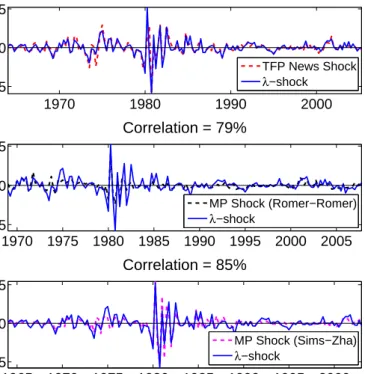
In fact, as shown by Figure1, the correlation between theλ-shock series and theTFP news shock series, estimated by Kurmann and Otrok (2013), and the monetary policy shock series identified by Romer and Romer (2004) and Sims and Zha (2006) is around 80%. This is striking given that my orthogonalisation strategy, as explained further below, has nothing to do with the strategies used to identify monetary policy or TFP news shocks, as my VAR model does not even contain a measure of TFP as an observable.
When applying the method to other equity portfolios such as size-operating profitability or size-investment or to a cross-section of US treasury bonds with different maturities, I find that the economic properties of the λ-shock are largely unchanged. Moreover, using the test assets constructed by Dimson, Nagel, and Quigley (2003) for the UK that are comparable to those constructed by Fama and French (1993) for the US, I find that the properties of the λ-shock are similar across the two countries.
Figure 1: The λ-shock and Well-known Structural Shocks
1970 1980 1990 2000 −5 0 5 % Correlation = 79% TFP News Shock λ−shock 1970 1975 1980 1985 1990 1995 2000 2005 −5 0 5 % Correlation = 79% MP Shock (Romer−Romer) λ−shock 1965 1970 1975 1980 1985 1990 1995 2000 −5 0 5 % Correlation = 85% MP Shock (Sims−Zha) λ−shock
Notes: The construction of theλ-shock is explained in Section2. The TFP news shock series are the ones plotted in Figure 5 on pp. 2625 ofKurmann and Otrok(2013) who apply the method ofUhlig(2004) to identify a TFP news shock over the period 1959Q2-2005Q2. The monetary policy shock series in the middle panel are originally proposed byRomer and Romer(2004) and updated byTenreyro and Thwaites(2016) to the period 1969Q1-2007Q4. The monetary policy shock series in the bottom panel are fromSims and Zha(2006) as documented inStock and Watson(2012).
In contrast, the obtained macroeconomic shock is markedly different when using the same VAR model but applying the orthogonalisation method to momentum portfolios. In this case, theλ-shock induces reactions in consumption, the interest rate and the term spread that are of opposite sign compared to theλ-shock implied by the FF25 portfolios. These results confirm the recent findings by Lettau, Ludvigson, and Ma (2017) and suggest that momentum premia are inversely exposed to the “macroeconomic, aggregate, nondiversifiable risk proxied by the returns of the HML and SMB portfolios”.
The Orthogonalisation Strategy The starting point of my analysis is a standard VAR including a small set of macroeconomic variables. The finance literature often
used Cholesky decomposition to obtain triangularised innovations in the spirit of the Intertemporal CAPM (Merton, 1973)1. Triangularisation is merely one of the infinite number of identification strategies to transform the reduced-form variance-covariance matrix to a structural form. I build on this point by exploring the entire space of possible orthogonalisations, given the estimated time-series of reduced-form residuals, with the aim to find the best approximation of the SDF from linear combinations of these residuals. Mechanically, the λ-shock is constructed as the one that, if used as a factor in the two-pass procedure of Fama and MacBeth (1973) applied to the given test portfolios, would generate the highest estimated factor risk premium in absolute value.
My approach does not make any of the assumptions that macroeconometricians tend to make when identifying structural shocks, e.g. restrictions regarding the short/long-run effects of the shock, or regarding the shock’s contribution to the forecast error variance (FEV) of a target variable in the VAR over a pre-specified horizon. Compared to these approaches, my method can be thought of as much more agnostic. Hence, there is no direct reason to believe that the obtained structural λ-shock should capture any of the economic forces studied by the structural VAR literature. The fact that it does, by closely resembling the statistical features of well-known macroeconomic shocks, could provide strong evidence on the relevance of those shocks in not only driving business cycles but also in explaining the cross-section of stock returns.
In addition, approximating the SDF with VAR residuals may have a possible advan-tage over standard no-arbitrage methods of estimating the SDF. The VAR framework and its rich machinery allows one to explore the link between the SDF and macroeconomic dynamics in more detail, making full use of the traditional macroeconometric toolkit. Impulse response function (IRF) analysis can be used to estimate how the λ-shock prop-agates through the economy in comparison with structural shocks traditionally identified in the macroeconomic literature. FEV decomposition can be used to estimate the con-tribution to business cycle dynamics of shocks that do not demand risk compensation, according to the given test portfolios, compared to shocks that do (λ-shock). These are just two of the examples of how the proposed framework can potentially provide a better understanding of the links between asset prices and business cycles.
Related Literature My paper is related to the finance literature on finding macroeco-nomic factors that drive the cross-sectional variation of risk premia. A partial list includes
Chen, Roll, and Ross (1986), Ferson and Harvey (1991), Campbell (1996), Cochrane
(1996),Vassalou(2003),Brennan, Wang, and Xia(2004),Petkova(2006),Liu and Zhang
(2008), Maio and Santa-Clara (2012), Koijen, Lustig, and van Nieuwerburgh (2012),
Boons and Tamoni (2015), He, Kelly, and Manela (2017). In addition, consumption based asset pricing (CCAPM) models also had success in explaining the cross-section of
returns by introducing conditioning variables (Jagannathan and Wang 1996; Lettau and Ludvigson 2001; Lustig and Nieuwerburgh 2005; Santos and Veronesi 2006; Yogo 2006) or focusing on the long-run component of consumption risk (Bansal and Yaron 2004;
Parker and Julliard 2005;Hansen, Heaton, and Li 2008;Constantinides and Ghosh 2011;
Bryzgalova and Julliard 2015).
A number of recent papers explored factors that are less reduced-form and are more tied to macroeconomic primitives. Modern macroeconomic models interpret business cy-cles as the outcome of simultaneous realisations of various structural disturbances with potentially very different quantities and prices of risk (Smets and Wouters 2007; Jus-tiniano, Primiceri, and Tambalotti 2010; Rudebusch and Swanson 2012; Borovicka and Hansen 2014; Campbell, Pflueger, and Viceira 2015; Greenwald, Lettau, and Ludvigson 2015; Ludvigson, Ma, and Ng 2015; Kliem and Uhlig 2016). In this spirit, more recent explanations of the cross-sectional variation of returns involve macroeconomic surprises related to monetary policy (Weber 2015;Ozdagli and Velikov 2016) and production tech-nology (Papanikolaou 2011; Kogan and Papanikolaou 2014; Garlappi and Song 2016) among others. My paper builds on these developments, and the results from applying my orthogonalisation strategy to the FF55 portfolios are consistent with the empirical findings of these two literatures.
Further, the method I propose builds heavily on the structural VAR literature (Sims 1980;Stock and Watson 2001). More specifically, the implementation of my orthogonali-sation theme draws on the more recent identification themes that use sign restrictions to identify structural shocks (Uhlig 2005;Rubio-Ramirez, Waggoner, and Zha 2010;Fry and Pagan 2011). As mentioned, finance papers using VARs (Campbell,1996;Petkova,2006;
Boons, 2016) typically applied Cholesky decomposition to the estimated reduced-form variance covariance matrix. While the obtained innovations had success in explaining the cross-section of returns, it has been difficult to assign macroeconomic interpretations to these innovations. Moreover, the idea of using observed asset prices to select a struc-tural shock draws on the long-standing literature of no-arbitrage estimation of the SDF (Hansen and Singleton 1982; Ait-Sahalia and Lo 2000;Rosenberg and Engle 2002; Cher-nov 2003; Ross 2015; Ghosh, Julliard, and Taylor 2016). Building on these papers, my method to explore the entire space of possible orthogonalisations in a VAR and to find the structural shock based on approximating the SDF given a set of portfolios is, to the best of my knowledge, novel in the literature.
Structure of the Paper The remainder of the paper is as follows: Section2 explains my empirical approach, Section3 presents the empirical results and Section4 concludes.
2
The Econometric Framework
2.1
The Geometry of the
λ
-shock
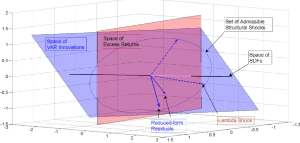
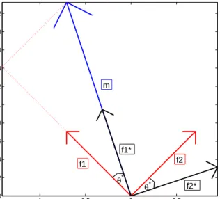
Before presenting the VAR model, it is instructive to first summarise the intuition behind finding the λ-shock. To do so and to highlight the geometrical nature of the ideas, I try to map some of the relevant mathematical background into a simplified 3-dimensional graph shown in Figure 2. There is an underlying probability space, and L2 denotes the
collection of all random variables with finite variances defined on that space. L2 is a
Hilbert-space with the associated norm kpk = (E(p2))1/2 for p∈ L
2. Let P denote the
space of portfolio excess returns (zero-price payoffs) that is assumed to be a closed linear subspace of L2.2 P is represented by the red plane in Figure2. An admissible stochastic discount factor is a random variable m in L2 such that the inner product of the excess
return and m satisfies 0 = E(mp) for all p∈P. The set of all admissible SDFs denoted by M is represented by the black line which goes through the origin and perpendicular to the red plane in Figure 2.3
Figure 2: A Simplified Geometry of Finding theλ-shock
Let S denote the set of reduced-form innovations from a VAR (the blue solid arrows in the Figure) and denote D the space spanned by these innovations. D is assumed to be a closed subspace of L2, and it is represented by the blue plane in the Figure.
The Gram-Schmidt orthogonalisation procedure allows the reduced-form innovations that span D to be transformed into a set of orthonormal vectors that also span D. The blue
2SeeHansen and Jagannathan(1991,1997) for a detailed discussion.
3As is well known, all SDFs can be represented as the sum of the minimum norm SDFs (the intersection
of the black line and the red plane in Figure2) and of a random variable that is orthogonal to the space
dashed arrows in Figure 2 represent two possible elements of the infinite sequence of orthogonalisations. The set of the all admissible orthogonalisations is denoted by O and is represented by the blue circle with unit radius in the Figure.
The space of VAR innovations is unlikely to contain an SDF because of model mis-specification or measurement error associated with observing SDFs (Roll(1977)). Loosely speaking, the tilted nature of the blue plane prevents all elements of O to be orthogonal to the space of excess returns, i.e. M ∩O =∅. Nevertheless, one can find an element in O that is closest to M in the spirit of Hansen and Jagannathan (1997) by applying the classical Projection Theorem.4 This has important implications for linear models of the SDF that use structural innovations from VAR models as pricing factors: there is one
particular orthogonalisation of the reduced-form VAR residuals that delivers a structural shock, which is closer to the SDF than all the other structural shocks in the VAR. This is the blue arrow labelled as the λ-shock in Figure 2, whose projection onto the space of SDFs is the magenta line. Given that this shock is the best possible approximation of the SDF, it summarises all the relevant information contained in all the reduced-form residuals of the VAR model. The next proposition for the two-dimensional case highlights that it is in fact easy to find the rotation which generates the λ-shock.
Proposition 1 Given the linear combination: m =af1+bf2, where a, b∈R, m, f1, f2 ∈ R2, kf1k=kf2k= 1 and hf1, f2i= 0, there exists a rotation rθ =
cosθ −sinθ sinθ cosθ with
0< θ <2π such that m=a?f1?+b?f2?, where a? 6= 0, b? = 0 and fi? =rθfi for i= 1,2.
While the proposition may seem a trivial piece of linear algebra (see Section A of the Appendix), it has important implications for using orthonormalised shocks from VAR models as pricing factors in linear pricing models. It is a well known theorem that beta pricing models are equivalent to linear models for the SDF (pp. 106-107Cochrane(2005)). Denoting the SDF, the pricing factor, the excess returns and the first- and second-stage regression coefficients from a linear pricing model by m, f, Re, β and λ, respectively, I
re-state the version of the theorem when the test assets are all excess returns:
Theorem 2 (Cochrane 2005) Given the model
m = 1 + [f−E(f)]0b 0 =E(mRe),
(2.1)
one can find λ such that
E(Re) = β0λ, (2.2)
4That is, assuming thatO is a complete linear subspace ofH, there exists a unique vectorm 0∈O,
corresponding to any vector x∈ M, such that kx−m0k ≤ kx−mk for allm ∈ O. See pp. 50-51 of
Luenberger(1969) for a classic treatment and pp. 608-609 ofHansen and Richard(1987) for a conditional version of the theorem.
where β are the multiple regression coefficients of excess returns Re on the factors. Con-versely, given λ in 2.2, we can findb such that 2.1 holds.
It is shown by Cochrane(2005) that λ and b are relatedλ=−var(f)b. This result sim-plifies greatly when working with pricing factors (such as orthonormalised VAR residuals) that have zero mean and unit variance. In this case,λ =−b and E(f) = 0.
The following section will highlight that finding the orthonormalised shock in a VAR of any dimension that demands the highest price of risk (λ) when pricing a given portfolio of assets is equivalent to finding a single time series that is a linear combination of the reduced form innovations of the VAR which summarises all the information relevant to pricing the given portfolio.5 More importantly, it is then possible to apply the struc-tural VAR methodology to learn about the causal effect of the shock on macroeconomic dynamics.
2.2
The VAR Model
Given aK×1 time series denoted byXt, thep-th order structural VAR can be represented
as follows6: Xt =k+A1Xt−1+A2Xt−2 +· · ·+ApXt−p+HΣet et ∼(0, IK), Σ = σ11 0 . . . 0 0 σ22 0 0 .. . ... . .. 0 0 0 . . . σKK , σjj ≥0 ∀j, (2.3)
where the structural shocksethave zero mean, unit variance and are serially and mutually
uncorrelated. Knowing the structural form2.3 would be useful for both asset pricing and macroeconomic purposes. For example, the asset pricing literature (Cochrane,2011) may want to see whether elements of et can explain risk premia, whereas the macroeconomic
literature (Sims, 1980) tends to focus on the causal effects of components of et on the
VAR dynamics. The latter is typically done by writing out the M A(∞) representation of 2.3:
Xt=µ+ Ψ (L)HΣet, (2.4)
where Ψ (L) is a lag polynomial of infinite order. The dynamic effects of structural shocks can then be studied by computing impulse response functions (IRF), ∂XT+s/∂ejt. The
reduced form corresponding to the structural form representation (2.3–2.4) can be written 5Another way of saying this is that the cross-sectionalR2-measure associated with a pricing model
that includes all the reduced-form residuals from the VAR is the same as the R2-measure associated with the one-factor model which uses the appropriately orthonormalised shock. This will be confirmed during the empirical application of the method (Panel A and B of Tables2–5.)
as:
Xt=µ+ Ψ (L)ηt
ηt∼(0,Ω), Ω =E(ηtηt0),
(2.5) whereηt are the reduced form innovations that are related to the structural shockset by
an invertible matrix H:
ηt=HΣet≡Bet, (2.6)
As is well-known in the literature, structural VARs (2.3) are not identified. The data provides information about the reduced form (2.5), but this information is not sufficient to uniquely determine the elements of B. Estimates of ηt and Ω provides k(k+ 1)/2
pieces of information about B, hence k(k−1) 2 additional restrictions are necessary to fully identify B. Sims (1980) originally proposed applying Cholesky decomposition to the reduced form variance covariance matrix (B = chol(Ω)) to obtained a unique, triangularise structure in the spirit of Wold (1954). This was subsequently used in the asset pricing literature as well (Campbell, 1996; Petkova, 2006; Boons, 2016). Over the last decades, a plethora of new techniques have been proposed to provide full or partial identification ofB, which involved both point and set identification of the elements ofB.7 Having introduced the VAR terminology, the method proposed in this paper essentially finds the elements of a single column of B which can be used to estimate the causal effect of an orthogonal macroeconomic shock which is the best approximation of the SDF according to a given cross-section of test assets. The following example highlights the intuition.
Example 3 (A Two-variable VAR Model) LetR be aT×n matrix of excess returns of n test portfolios. Take a two-variable VAR model (k = 2) and suppose that the pricing factors are the orthonormalised shocks implied by Cholesky decomposition (ft= [f1t|f2t] =
ηtB−1 = ηt(chol(Ω))
−1
). Given a linear pricing model 2.2, the estimated model for the SDF (m) is written as a linear combination of the two innovation series:
mt=λ1f1t+λ2f2t, (2.7) where λ1 and λ2 are the estimated prices of risk associated with f1 and f2. The λs can easily be obtained with the two-stage procedure ofFama and MacBeth(1973): (i) estimate
n time series regressions,Rit =ai+ftβi+it, i= 1. . . n, and (ii) estimate a cross-section regression, R¯i = ˜βi×λ+αi, where R¯i = T1 PTt=1Rit, β˜i is the OLS estimate obtained in the first stage and αi is a pricing error. Because f1 ⊥f2 and var(f1) =var(f2) = 1, the variance of the SDF is simply the sum of the squared values of the estimates of prices of
7See Kilian and Lutkepohl (2016), Ramey (2016) and Ludvigson, Ma, and Ng (2017) for a recent
risk associated with each one of the two VAR shock series:
var(mt) = λ21+λ 2
2. (2.8)
Rotation does not affect the overall information content in the VAR, that is, the volatility of the implied SDF is determined by the specification of the VAR and not by rotating the variance-covariance matrix of the residuals. The main implication of proposition 1is that the information contained in the VAR residuals can be summarised by merely one structural shock after applying an appropriate rotation to the variance-covariance matrix. To put it simply, there exists a rotation rθ =
cosθ −sinθ sinθ cosθ
such that using fi? =rθfi fori= 1,2as pricing factors, one of the estimated prices of risk would beλ?1 =qvar(m), as the other one corresponding to the rotated factorf2? would be zero λ?2 = 0. This implies that the best approximation of the SDF is found, f1? =m, and rθ can be used to perform structural analysis in the VAR, i.e. the corresponding column of the new structural impact matrix B? =Brθ can be used to compute IRFs.
It is important to note that finding rθ is of course not needed to find the time-series
λ-shock. Applying the Fama and MacBeth(1973) procedure to any set of orthonormalised residuals from a VAR will produce a unique time-series of theλ-shock that can be obtained as the fitted values of the second-stage regression. This is highlighted by lemma 6 of the Appendix. A linear model of the SDF, that uses arbitrarily orthonormalised VAR residuals, uniquely pins down one of the rows of the matrix (B?)−1. However, this in itself is not sufficient to carry out structural VAR analysis, because to do so one needs to know the column in the structural impact matrix B? (and not its inverse (B?)−1) that corresponds to the λ-shock. Building on the example above, the following proposition establishes the relationship between the angle θ needed to compute the IRFs associated with the λ-shock.
Proposition 4 Given the two-variable VAR model described above with a reduced form variance-covariance matrix Ω = ω11 ω12 ω12 ω22 , the column of B? = B11? B12? B21? B22? corre-sponding to the contemporaneous effect of the λ-shock is given by:
B?11=√ω11cos (θ)
B?21= √ω12
ω11
cos (θ) +qω22−ω122 /ω11sin (θ)
(2.9)
with the rotation angleθ determined by the estimated prices of risks,θ= arcsinλ2/ q
(λ2 1+λ22)
.
Example 5 (A Two-variable VAR and the Consumption-CAPM) Let the two vari-ables in a quarterly VAR(2) be the log of consumption and the term spread, and let the test assets be the 25 Fama-French (FF25) portfolios. An OLS regression using data from 1970Q1 to 2012Q2 yields an estimated variance-covariance matrixΩ =ˆ
0.38 −0.07 −0.07 0.78 . Following the calculations in Proposition (4), the given test assets and the reduced-form residuals, uC
t and uT ermt , imply the following estimated model of the SDF:
mt = 0.21uCt + 1.14u T erm t ,
which suggests that reduced-form innovations in the term-spread load substantially more than reduced-form consumption innovations. The difference is much more striking when looking at the contemporaneous impact of the shock on consumption and the term spread. Using the appropriate angle θ, the elements of the B? are as follows:
ˆ
B11? = 0.006 Bˆ12? = 0.61 ˆ
B21? = 0.88 Bˆ22? =−0.12.
(2.10)
The values in the first column suggest that a one standard deviation λ-shock induces a large (0.88%-points) immediate jump in the term spread, but the shock has virtually no contemporaneous effect (<0.01%) on consumption. This confirms the results of recent Consumption-CAPM models (Bryzgalova and Julliard, 2015) as discussed further below. Moreover, the second column shows the contemporaneous effect of the second shock in the system that is by construction orthogonal to the SDF implied by FF25 portfolios and VAR model (the λ-shock) and thereby demands zero risk premia. This shock has a large (0.61%) contemporaneous effect on consumption which implies that virtually all of the one period ahead forecast error variance in consumption is explained by a shock, exposure to which demands zero risk compensation according to the FF25.
3
The Empirical Results
3.1
VAR Estimation and Data
To implement the orthogonalisation strategy in a larger model, I start by estimating the n-variable reduced-form VAR (2.5) and applying Cholesky decomposition to the estimated variance-covariance matrix ˆΩ = ˆBBˆ0 where ˆB is lower triangular. As discussed, one can take any orthonormal matrix Q to obtain a new structural impact matrix ˆB? = ˆBQ, thereby obtaining a new set of structural shocks, which conforms to the reduced-form variance covariance matrix, i.e. ˆΩ = ˆB?Bˆ?0 = ˆBQBˆQ0 = ˆBBˆ0. To find Q which delivers the unique column in ˆB? corresponding to the contemporaneous impact of the
λ-shock, I span the space of n-dimensional orthonormal matrices that are rotations with an n-dimensional Givens rotation.8 I choose the Euler-angles of the Givens rotation appropriately such that, given the test assets, the correspondingλestimate in the second-pass Fama and MacBeth (1973) regression is maximised. The construction of the Q matrix is described in Section B of the Appendix.
To operationalise the VAR model, one needs to specify the variables to be included in the state vector. I opt for a parsimonious model with the following five (n = 5), com-pletely standard state variables: aggregate consumption, aggregate price level, the policy interest rate, the default spread and the term spread. Consumption is measured as total personal consumption expenditure as inGreenwald, Lettau, and Ludvigson(2015). Data on the following three series are from the Federal Reserve Bank of St. Louis (FRED): output is measured as quarterly seasonally adjusted real GDP (FRED code: GDPC1), price level is measured as the personal consumption expenditures (chain-type) price index (FRED code: PCEPI), the policy interest rate is the Federal Funds Rate (code: FED-FUNDS) and the default spread is the difference between the AAA (FRED code: AAA) and BAA (FRED code: BAA) corporate bond yields. The term spread is defined as the difference between the long term yield on government bonds and the T-bill as used in
Goyal and Welch (2008). These five variables have long been recognised as good candi-dates for state variables within the ICAPM framework, and they frequently appear as key variables in macroeconomic forecasting models as well. When estimating the VAR, I deliberately avoid using financial variables such as aggregate excess returns or various valuation ratios, that are known to increase the overall fit of cross-sectional asset pricing models. The specification of the state vector is motivated by the desire to stay as close as possible to macroeconomic explanations of the cross-section of stock returns, in the spirit of Chen, Roll, and Ross (1986) and subsequent papers. The baseline VAR model includes two lags as suggested by the Schwarz Information criterion.
The sample period for the estimation is 1963Q3-2008Q3 and the data are at quarterly frequency. The start of the estimation period is chosen by the majority of empirical asset pricing studies of the cross-section. The end of the estimation period is chosen to exclude the Great Recession period when the Federal Funds Rate hit the zero-lower bound. As for the FF55 portfolios, 25 of them (FF25 henceforth) are formed from independent sorts of stocks into five size groups and five B/M groups as described in Fama and French
(1993). The other 30 portfolios are four-digit SIC code level industry portfolios. The monthly returns in excess of the one-month U.S. Treasury bill rate are transformed into quarterly series. As studied extensively by the empirical asset pricing literature, average returns typically fall from small stocks to big stocks (size effect), and they rise from portfolios with low to large book-to-market ratios (value effect). Augmenting the FF25 with the 30 industry portfolios follows prescription 1 (pp. 182) of Lewellen, Nagel, and
Shanken (2010), thereby relaxing the tight factor structure of Size-B/M. Moreover, I apply the orthogonalisation method to additional test portfolios such as the 25 portfolios sorted on size and operating profitability, the 25 portfolios sorted on size and investment, and the 10 momentum portfolios sorted on the cumulative returns of stocks from 12 months before to one month before the formation date using a one-month gap before the holding period. All the portfolios are value-weighted and are taken from Ken French’s data library. As an alternative, I also use the 10 momentum portfolios as constructed in
Daniel and Moskowitz(2016).9
3.2
The Economic Characteristics of the
λ
-shock
Using the OLS estimates of the VAR, I compute impulse response functions (IRF) after performing the orthogonalisation strategy described in Section 2. This is to understand the macroeconomic impact of the λ-shock which is by construction the structural shock that best approximates the SDF given the 5-variable VAR(2) model and the FF55 port-folios. Section D of the Appendix describes a Bayesian treatment of the computation of the IRFs in order to explore the role of parameter uncertainty in the VAR model.
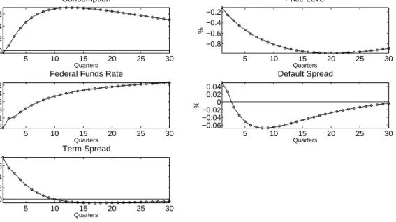
Figure 3: Impulse Responses to a λ-shock
5 10 15 20 25 30 0 0.2 0.4 0.6 Quarters Consumption % 5 10 15 20 25 30 −0.8 −0.6 −0.4 −0.2 Quarters Price Level % 5 10 15 20 25 30 −1.2 −1 −0.8 −0.6 −0.4 −0.2 Quarters
Federal Funds Rate
% 5 10 15 20 25 30 −0.06 −0.04 −0.02 0 0.02 0.04 Quarters Default Spread % 5 10 15 20 25 30 0 0.2 0.4 0.6 Quarters Term Spread %
Notes: The vertical axes are %-deviations from steady-state, and the horizontal axes are in quarters.
Figure3displays the IRFs of the five variables to a one standard deviation structural innovation. The term spread jumps by about 70 basis points on impact and there is a 9As explained inDaniel and Moskowitz(2016) the biggest difference is that the portfolio breakpoints
for the portfolios constructed by Ken French are set so that each of the portfolios has an equal number of NYSE firms. In contrast,Daniel and Moskowitz (2016) set their breakpoints so that there are an equal number of firms in each portfolio. This mainly affects the low-momentum returns.
very sharp and persistent drop in the Federal Funds Rate. The initial drop in the price level is lower than the drop in the Federal Funds Rate, suggesting a sharp drop in the real interest rate. Interestingly, the λ-shock has virtually no effect on GDP on impact, but the effect increases substantially with the horizon from the third quarter onwards and reaching a peak impact of about 0.7% approximately 12-15 quarters after the shock hits. As shown by Figure10in the Appendix, the shape of these IRFs is similar when the lag length is changed or when output is replaced by consumption in the VAR. A robust finding is that the λ-shock does not trigger a positive comovement between consumption and the short-term interest rate that is generated by most demand-type shocks proposed by the recent macroeconomic literature (Christiano, Motto, and Rostagno,2014).
To assess the contribution of the λ-shock to business cycles, in comparison with other structural shocks that have zero covariance with the implied SDF, I compute FEV de-composition over different horizons. Table 1 shows that the λ-shock explains about 1% of consumption fluctuations over the six-month horizon, but the shock explains around 50-65% of fluctuations over longer (4-9 years) horizon. While these number are substan-tial, there is some unexplained fraction of output fluctuations that is driven by structural shocks exposures to which do not demand risk compensation according to the given test assets. Moreover, Table 1 also shows that the λ-shock drives around 70-80% of interest
Table 1: The Contribution of the λ-shock to Business Cycles: FEV Decomposition
Consumption CPI FFR Def. Spread Term Spread
2Q 1.3 15.8 85.8 8.4 73.1 4Q 13.3 22.2 83.1 8.2 72.3 8Q 38.3 30.1 80.4 21.0 70.3 16Q 50.6 34.6 79.2 29.2 69.4 24Q 62.1 39.6 78.2 34.2 68.8 36Q 64.7 40.1 78.0 34.2 68.6
Notes: The table shows the % fraction of the total forecast error variance that is explained by theλ-shock over different forecast horizons. The FF55 portfolios are used as test portfolios for the VAR model.
rate and term spread fluctuations and around 20-40% of fluctuations in the aggregate price level and the default spread. The explained variation in the FEV in the interest rate and the term spread seems to decrease over the forecast horizon, whereas it increases for consumption, the price level and the default spread.
To place these results in the literature, the delayed response of aggregate consumption in response to innovations that are relevant to asset pricing is a phenomenon that has been documented by the consumption based macro-finance (Parker and Julliard, 2005) and long run risk literatures (Bansal and Yaron, 2004). More recently, Bryzgalova and Julliard(2015) have shown that “slow consumption adjustment shocks” account for about a quarter of the time series variation of aggregate consumption growth, and its innovations explain most of the time series variation of stock returns. My results are consistent with their findings. In addition, my multivariate time-series framework is somewhat richer
than their reduced-form consumption growth model, so it can possibly shed further light on the macroeconomic drivers of the slow consumption adjustment shocks that are the main source of aggregate risk.
One possible interpretation of Figure 3is that theλ-shock behaves like a supply-type shock with aggregate quantities moving in the opposite direction compared to the price level and the short-term interest rate. However, the delayed expansion of consumption would make the λ-shock clearly distinct from a positive unanticipated technology shock which would have an immediate positive impact on output and consumption, as tradi-tionally studied by the Real Business Cycle (RBC) and the subsequent New Keynesian literature.10 However, a news-type technology shock that typically triggers a delayed reaction in aggregate quantities may be perfectly consistent with Figure 3.11 Indeed, Figure 4 of Kurmann and Otrok (2013) shows results for an identified TFP news shock with very similar IRFs to mine. The striking similarity between my Figure 3 and their findings occurs in spite of the fact that they identify a TFP news shock, followingBarsky and Sims (2011), by searching for a shock that accounts for most of the forecast error variance of TFP over a given forecast horizon, and they force this shock to be orthogonal to contemporaneous movements in TFP.
An alternative interpretation of Figure 3 is that a positive λ-shock behaves like an expansionary monetary policy shock to the extent that it generates an immediate jump in the short-term interest rate and the term spread and a delayed but persistently ex-pansionary reaction in output. Though CPI goes the ’wrong’ way, but it is somewhat consistent with the ’price puzzle’ (Sims,1992) associated with early methods of Cholesky orthogonalisation to identify monetary policy shocks as in Christiano, Eichenbaum, and Evans (1999) and others.
To formally show the similarity between the λ-shock and some well-known structural shocks studied by macroeconomists, Figure 1 in the Introduction plots the time-series of the λ-shock against the TFP news shocks identified by Kurmann and Otrok (2013) (upper panel) and against the monetary policy shocks identified by Romer and Romer
(2004) (lower panel). Based on the overlapping estimation period 1963Q4–2005Q2, the correlation coefficient between the TFP news shock series (red dashed line) as identified 10Though technology shocks had some theoretical success in explaining aggregate excess returns in an
RBC framework (Jermann, 1998), the most recent empirical evidence by Greenwald, Lettau, and Lud-vigson(2015) finds that the contribution of unanticipated TFP shocks to the variance of aggregate stock market wealth is close to zero. These authors identify three mutually orthogonal observable economic disturbances that are associated with over 85% of fluctuations in real quarterly stock market wealth. They find that the third triangularised shock from a cointegrated three-variable VAR (including con-sumption, labor income, and asset wealth) is the main driver of the variance of aggregate stock market wealth. Their identifying assumption implies zero contemporaneous impact on consumption – an as-sumption that is consistent with the IRF results implied by the more agnostic orthogonalisation theme adopted in this paper.
11A partial list of the rapidly increasing macroeconomic literature on news shocks includes Beaudry
and Portier (2006, 2014), Jaimovich and Rebelo (2009), Barsky and Sims (2011), Schmitt-Grohe and Uribe(2012),Kurmann and Otrok(2013),Malkhozov and Tamoni(2015).
in Kurmann and Otrok (2013) and the λ-shock series (blue solid line) is 0.79. Based on the overlapping estimation period 1969Q1–2007Q4, the correlation coefficient between the monetary policy shock series (black dashed line) as identified in Romer and Romer
(2004) (and updated by Tenreyro and Thwaites (2016)) and the λ-shock series is 0.79. The correlation with the monetary policy shock series identified by Sims and Zha(2006) is 0.85 over the period 1963Q4–2003Q1.
To reiterate, my orthogonalisation strategy is unrelated to those frequently used in the macroeconomic literature as it (i) makes no assumption about theλ-shock’s contribution to the forecast error variance of any of the variables like Kurmann and Otrok (2013) does12, (ii) does not rely on any narrative measures such as FOMC records like Romer
and Romer(2004) does, (iii) does not impose any zero-type or sign restrictions like Sims and Zha (2006) does and (iv) does not even include TFP as an observable in the VAR. Not to mention the additional differences of my empirical model in terms of lag structure, sample period and variables used in the VAR. The fact that I come close to reconstructing the object the TFP news literature and the monetary policy literature have studied (by applying a completely different and relatively more agnostic methodology) could provide strong empirical support for the relevance of these shocks in driving business cycles as well as asset price dynamics.
3.3
Extensions
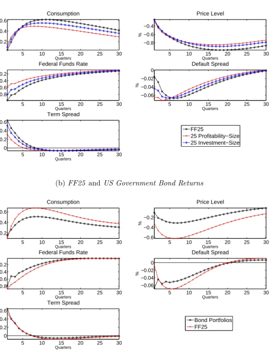
Other Equity Portfolios and Government Bond Returns To check the robustness of the findings above, I explore how the behaviour of the λ-shock changes when the same VAR model and the orthogonalisation method are applied to other test assets. A natural choice is the 25 portfolios double sorted on size-profitability and size-investment. These portfolios feature prominently in the most recent empirical asset pricing studies (Fama and French, 2015, 2016). In addition, I also compute the IRFs for the λ-shock implied by the benchmark FF25 portfolios, sorted on size-B/M, that have been the most studied test assets to date.
The upper panel of Figure 4 shows the IRFs for these three sets of equity portfolios. The results suggest that the economic behaviour of theλ-shock implied by these portfolios is very similar to the λ-shock implied by the baseline FF55 as shown in Figure 3. The only quantitative difference is that the baseline results imply a larger peak effect on consumption and a more delayed effect on the default spread compared to Figure 4.
Moreover, I also use government bond returns that are calculated using the zero coupon yield data constructed by Gurkaynak, Sack, and Wright (2007) that fit Nelson-Siegel-Svensson curves on daily data. The parameters for backing out the cross-section 12The latter type of restriction has been increasingly popular (since its development byUhlig(2004)),
Figure 4: Impulse Responses to a λ-shock, Implied by other Equity Portfolios and Gov-ernment Bond Returns
(a)FF25, 25 Profitability-Size and 25 Investment-Size Portfolios
5 10 15 20 25 30 0.2 0.4 0.6 Quarters Consumption % 5 10 15 20 25 30 −0.8 −0.6 −0.4 Quarters Price Level % 5 10 15 20 25 30 −0.8 −0.6 −0.4 −0.2 Quarters
Federal Funds Rate
% 5 10 15 20 25 30 −0.06 −0.04 −0.02 0 Quarters Default Spread % 5 10 15 20 25 30 0 0.2 0.4 0.6 Quarters % Term Spread FF25 25 Profitability−Size 25 Investment−Size
(b)FF25 and US Government Bond Returns
5 10 15 20 25 30 0.2 0.4 0.6 Quarters Consumption % 5 10 15 20 25 30 −0.6 −0.4 −0.2 Quarters Price Level % 5 10 15 20 25 30 −0.8 −0.6 −0.4 −0.2 Quarters
Federal Funds Rate
% 5 10 15 20 25 30 −0.06 −0.04 −0.02 0 Quarters Default Spread % 5 10 15 20 25 30 0 0.2 0.4 0.6 Quarters % Term Spread Bond Portfolios FF25
Notes: The vertical axes are %-deviations from steady-state, and the horizontal axes are in quarters. The upper panel uses the VAR(2), as estimated in Subsection3.2, and employs alternative equity portfolios to the construction of the
λ-shock. The lower panel estimates the same VAR(2) on a subsample 1975Q2-2008Q3, and employs the FF25 and holding period excess returns on 18 US treasury bonds with different maturities.
of yields are published on their website. The sample period is 1975Q2-2008Q3 so that I have sufficiently large cross-section of yields. I use maturities for n = 18,24, . . . ,120 months and compute one-month holding period excess returns which I then transform into quarterly series. The resulting 18 bond portfolios are used to construct the λ-shock. The lower panel of Figure4shows the results, confirming that the shock responsible for pricing equities is virtually identical to the shock that prices government bonds. This is consistent with the relatively small but growing literature on the joint pricing of stocks and bonds (Lettau and Wachter 2011; Koijen, Lustig, and van Nieuwerburgh 2012; Bryzgalova and Julliard 2015).
Adding More Variables to the VAR A natural extension of the baseline model is to add more variables to the VAR. One advantage of the present multivariate set-up is that one can use it as a unifiying framework to model the joint dynamics of any reduced-form variables that individually have been found to price the cross-section of returns, and to link the common stochastic driver of these variables to a single orthogonal shock.13
Figure 5 shows the results from an eight-variable VAR with each one of the eight variables individually found to be relevant to asset pricing: early studies (Sharpe, 1964) on the CAPM focused on the covariance with the market return, the consumption-CAPM and long-run risk literatures (Bansal and Yaron 2004; Parker and Julliard 2005; Hansen, Heaton, and Li 2008; Constantinides and Ghosh 2011; Bryzgalova and Julliard 2015;
Boons and Tamoni 2015) focused on specific innovations in the consumption process, the ICAPM (Chen, Roll, and Ross, 1986; Liu and Zhang, 2008) emphasised output inno-vations and also the role of the term spread and default spread (Hahn and Lee, 2006), inflation risk has also been proposed as an important pricing factor (Bekaert and Wang,
2010; Boons, Duarte, de Roon, and Szymanowska, 2013), and the balance sheet position of financial intermediaries has recently been proposed (He, Kelly, and Manela, 2017) as a key determinant of the pricing kernel.
As emphasised in the introduction, these variables are reduced-form objects and often exhibit high correlations with one another. For example, consumption innovations and output innovations extracted from individual AR(1) models have around 66% correlation, term spread innovation and federal funds rate innovations have around -82% correlation, the intermediary capital risk factor constructed by He, Kelly, and Manela (2017) and excess returns on the market (their second pricing factor) have a 78% correlation.14 A main finding of this paper is that the VAR framework and the rotation of the variance-13Increasing the size of the VAR introduces only computational challenges. For example, in an
8-variable (10-8-variable) VAR one needs to find 420 (4725) angles to span the 8-dimensional space of rotations. See sectionBof the Appendix.
14These number are based on estimates of individual AR(1) models on consumption, GDP, the term
spread and the Federal Funds rate covering the period 1963Q3-2008Q3. The correlation between the intermediary capital risk factor and market excess returns are for 1970Q1-2012Q4 as inHe, Kelly, and Manela(2017).
covariance make it possible to find a single, meaningful stochastic driver behind these reduced-form innovations.
Figure 5: Impulse Responses to a λ-shock
5 10 15 20 25 30 0 0.2 0.4 Quarters Consumption % 5 10 15 20 25 30 0 0.2 0.4 0.6 Quarters Output % 5 10 15 20 25 30 −0.6 −0.4 −0.2 Quarters Price Level % 5 10 15 20 25 30 −0.8 −0.6 −0.4 −0.2 Quarters
Federal Funds Rate
% 5 10 15 20 25 30 −0.04 −0.02 0 Quarters Default Spread % 5 10 15 20 25 30 0 0.2 0.4 0.6 Quarters Term Spread % 5 10 15 20 25 30 0.1 0.2 0.3 Quarters
Intermediary Capital Ratio
% 5 10 15 20 25 30 −0.5 0 0.5 1 Quarters
Market Excess Return
%
Notes: The vertical axes are %-deviations from steady-state, and the horizontal axes are in quarters. The VAR(2) is estimated on a subsample 1970Q1-2008Q3 given the availability of the intermediary capital ratio series ofHe, Kelly, and Manela(2017) that starts in 1970. I use the FF25 to construct theλ-shock.
Figure 5 confirms that all these variables respond to the λ-shock the way consistent with the papers mentioned above that tried to explain the FF25. Aggregate quantities react slowly, the intermediary equity capital ratio reacts sharply and persistently, realised excess returns jump on impact and revert in the next period, and the other variables behave similarly to the baseline model presented above. Overall, these results suggest that the average returns of the equity portfolios and bond returns studied so far can be explained by the different degrees of positive exposure to approximately a common source of macroeconomic risk. As shown in the next subsection, these results change markedly when using momentum portfolios to construct the λ-shock.
3.4
Momentum
Since it was first documented (Asness, 1994; Jegadeesh and Titman, 1993), momentum returns have been challenging to explain with pricing factors that worked well in pricing the traditional Fama-French portfolios. As a result, many linear factors models since
Carhart (1997) included a momentum factor explicitly in their pricing models in order to explain momentum. Even the most recent generation of pricing models such as the five-factor model ofFama and French(2015,2016) fail badly as descriptions of average returns on momentum portfolios without including a momentum factor in their model. This is
particularly puzzling given that momentum is a pervasive phenomenon that appears in many diverse markets and asset classes (Asness, Moskowitz, and Pedersen, 2013).
To explore the potentially different structural macroeconomic risks underlying mo-mentum portfolios, I apply the same VAR and orthogonalisation technique to the 10 momentum (Prior 2-12) portfolios constructed by Ken French and to the 10 momentum portfolios used in Daniel and Moskowitz (2016). Figure 6 shows the impact of a one standard deviation λ-shock implied by the momentum portfolios compared with the λ-shock implied by the FF55 portfolios. The results suggest that the λ-shock implied by momentum has a markedly different dynamic effect on the economy. Most of the IRFs flip sign compared to the λ-shock implied by the value and size portfolios.
Figure 6: Impulse Responses to a λ-shock, Implied byMomentum Portfolios
5 10 15 20 25 30 −0.2 0 0.2 0.4 0.6 Quarters Consumption % 5 10 15 20 25 30 −0.8 −0.6 −0.4 −0.2 0 Quarters Price Level % 5 10 15 20 25 30 −1 −0.5 0 0.5 Quarters
Federal Funds Rate
% 5 10 15 20 25 30 −0.05 0 0.05 Quarters Default Spread % 5 10 15 20 25 30 −0.5 0 0.5 Quarters % Term Spread FF55 10 Momentum (FF) 10 Momentum (Daniel−Moskowitz)
Notes: The vertical axes are %-deviations from steady-state, and the horizontal axes are in quarters.
These results are in line with the recent evidence ofLettau, Ludvigson, and Ma(2017) who shows that momentum premia are inversely exposed to the factors that explain value and size. Relatedly, it is well known that momentum strategies and more traditional trading strategies such as value are negatively correlated.15 In the present framework this would suggest that the time-series of the macroeconomic shock exposures to which these two strategies have delivered large risk premia historically must be quite distinct. Indeed, the correlation between the time-series of theλ-shock implied by the FF55 portfolios and of the λ-shock implied by the 10 momentum portfolios of Ken French and Daniel and Moskowitz (2016) is -0.60 and -0.68, respectively.
15For example, Table I ofAsness, Moskowitz, and Pedersen(2013) shows that value and momentum
3.5
Pricing the Cross-section of Stock Returns
It is worth noting that the focus of this paper is not the asset pricing performance of the λ-shock. Conditional on the VAR model2.3 being an accurate representation of the economy, the λ-shock itself is the SDF by construction. Put it differently, the pricing performance of the givenλ-shock can easily be improved by changing the specification of the VAR (e.g. including additional variables such as the intermediary capital ratio ofHe, Kelly, and Manela(2017) as in Section3.3 or valuation ratios16) but not by changing the orthogonalisation assumption. Though the baseline five-variable macroeconomic VAR model is far from being an accurate representation of the economy, but it is a standard and parsimonious way of summarising macroeconomic dynamics.
For the interested reader, I do summarise in this subsection the asset-pricing perfor-mance of the λ-shock implied by each test portfolios studied above. As argued above, this only is a test as to whether the variables included in the VAR contain information relevant to pricing the given portfolios. Tables 2–5 of the Appendix present the results from the two-pass regression technique of Fama and MacBeth (1973). During this ex-ercise, I treat the uncovered λ-shock as a known factor when estimating the two-pass regression model. To estimate the risk premium associated with theλ-shock, I apply the GMM procedure described inCochrane (2005) and implemented by Burnside (2011).
Overall, the pricing performance of the VAR (or equivalently, the λ-shock) is com-parable with the 3-factor model of Fama and French (1993).17 Moreover, as explained in Section 2, finding the λ-shock implies that the other four structural shocks have zero covariance with the implied SDF, and therefore the associated estimated prices of risk are numerically zero, as shown in panel B of Tables 2–5. Relatedly, the R2 associated with the one-factor model using theλ-shock is identical to theR2 for the model using any set of five orthogonalised shocks or in fact the model which uses the five reduced-form VAR residuals.
Moreover, the results are also consistent with Lewellen, Nagel, and Shanken (2010) who pointed out the strong factor structure of the FF25 portfolios which makes it rela-tively easy to find factors that generate high cross-sectional R2s. Hence, they prescribed
to augment the FF25 with the 30 industry portfolios of Fama-French in order to relax the tight factor structure of the FF25. Indeed, the cross-sectional R2 drops drastically from 0.86 to 0.25 for the 1-factor model without a common constant, and it drops from 0.77 to 0.20 for the 3-factor model of Fama-French without a common constant. This can be interpreted as the relevant information content of the VAR being much smaller for pricing the FF55 portfolios than for pricing the FF25 portfolios. This may of course lead to a critique of the (lack of) relevant information content of the VAR for pricing the FF55
16These results are available upon request.
17Applying the 3-factor model to the FF25 portfolios (Table3) yields similar results to those obtained
portfolios, which may call for enriching the information set by adding valuation ratios to the VAR. Nevertheless, changing the VAR may be unnecessary because this poor pricing performance is unlikely to undermine the results of this application of my orthogonalisa-tion strategy: the macroeconomic shock that captures all relevant informaorthogonalisa-tion for pricing the cross section (irrespective of whether the information content is relatively small or large) bears virtually the same economic characteristics as the λ-shock using the FF25 portfolios. The IRFs are similar for the λ-shock using the FF25 and the FF55 (Figures3
and 4), and the time-series of the shocks implied by the two portfolios have a high (0.82) correlation coefficient.
3.6
The
λ
-shock and the Fundamentals
An application of my proposed orthogonalisation strategy to the stock portfolios of FF55 led to the result that the estimated λ-shock bears a close empirical relationship both with TFP news shocks and with monetary policy shocks. This ambiguity of the result might seem an awkward outcome: after all, how can the resulting λ-shock have such a high correlation with two, seemingly distinct structural disturbances? To convince the reader that this is not a fault of my orthogonalisation strategy, I propose one possible and simple explanation for such an ambiguity: TFP news shocks and monetary policy shocks are in fact highly correlated in the data.
To provide some suggestive evidence for this argument, I use the VAR model of
Kurmann and Otrok (2013) to identify a monetary policy shock using Cholesky orthogo-nalisation as done bySims (1980),Christiano, Eichenbaum, and Evans (1999) and many others in the monetary policy literature. In this case, I deliberately use exactly the same VAR specification as used by Kurmann and Otrok (2013) when they identified a TFP news shock so that I can learn about differences and similarities across the two iden-tification themes without changing the information set. The upper panel of Figure 7
plots the estimated time-series of the TFP news shocks (black dashed line) against the monetary policy shock series identified with Cholesky orthogonalisation (red solid line). The correlation between the two series is strikingly high (0.96), raising questions about the orthogonality of these shocks with respect to one another.
Of course, the identification of monetary policy shocks with Cholesky orthogonali-sation is only one of the many possible identification strategies. Therefore, I provide additional evidence from the structural model of Smets and Wouters (2007) which is a dynamic stochastic general equilibrium (DSGE) model estimated with Bayesian methods. Monetary policy shocks in this framework are the estimated innovations in a Taylor-type monetary policy rule. The estimated time-series of these structural innovations from the DSGE model are plotted in the lower panel of Figure 7(blue solid line) against the TFP news shocks (black dashed line) ofKurmann and Otrok (2013). The correlation between
Figure 7: Comparing TFP News Shocks against Monetary Policy Shocks: Results from
Kurmann and Otrok (2013)’s VAR and from Smets and Wouters(2007)’s DSGE Model.
1965 1970 1975 1980 1985 1990 1995 2000 2005 −6 −4 −2 0 2 Years % Correlation = 96%
Monetary policy shock Cholesky TFP news shock 1965 1970 1975 1980 1985 1990 1995 2000 −4 −2 0 2 Years % Correlation = 81%
Monetary policy shock Smets−Wouters (2007) TFP news shock
Notes: The TFP news shock series (black dashed line) are the ones plotted in Figure 5 on pp. 2625 ofKurmann and Otrok(2013) who apply the method ofUhlig(2004) to identify a TFP news shock over the period 1959Q2-2005Q2. The monetary policy shock series in the upper panel (red solid line) are identified with Cholesky identification as in
Christiano, Eichenbaum, and Evans(1999), using the same variables and lag length asKurmann and Otrok(2013). The monetary policy shock series in the lower panel (blue solid line) are the estimated time-series of innovations in the Taylor-rule in the DSGE model ofSmets and Wouters(2007).
these two series is still remarkably high (0.81).
I interpret these findings as confirmation that the somewhat ambiguous characteri-sation of the obtained λ-shock is not an outcome of the potential weakness of my or-thogonalisation theme, but it is a result of the high empirical correlation between the two, well-known structural disturbances that the λ-shock resembles. To the best of my knowledge, this empirical regularity has not been documented in the literature yet, and it could be subject to further research.
3.7
Results from the UK
To check whether the results are robust to countries other than the US, I re-estimate the λ-shock using data for the UK covering the period 1975Q1-2001Q4. One advantage of using data for the UK is related to the availability of both comparable monetary policy shock series and comparable test assets across the two countries in question. The accounting and share price information was collected by Dimson, Nagel, and Quigley (2003) which they used to construct test assets sorted on size-B/M over the 1955-2001 period. I use the 16 test assets (UK16) constructed by them, whereby breakpoints were applied to the 40th, 60th and 80th percentiles of market capitalisation and to the 25th, 50th and
75th percentiles of book-to-market.Their portfolio formation closely follows Fama and French (1993). The UK monetary policy shock series is taken from Cloyne and Hurtgen
(2016) that uses the methodology ofRomer and Romer(2004) to try to eliminate much of the endogenous movement between the interest rate and other macroeconomic variables as well as to control for the effects related to current expectations of future economic conditions. To keep the empirical model close to the US counterpart presented above, I estimate a VAR(2) model with five macroeconomic variables: log of consumption, log of CPI, the Bank of England policy rate, the unemployment rate and the term spread defined as the difference between the 10-year and 1-year constant maturity Gilt rates. The first four series are from the dataset of Cloyne and Hurtgen (2016), and the term spread are from the Bank of England database.
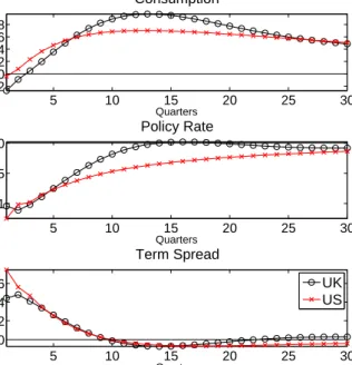
Figure 8: Comparing the Effect of theλ-shock: US vs UK
5 10 15 20 25 30 −0.20 0.2 0.4 0.6 0.8 Quarters Consumption % 5 10 15 20 25 30 −1 −0.5 0 Quarters Policy Rate % 5 10 15 20 25 30 0 0.2 0.4 0.6 Quarters % Term Spread UK US
Notes: The vertical axes are %-deviations from steady-state, and the horizontal axes are in quarters.
Figure8compares the IRFs for theλ-shock implied by the UK data to those presented by the US benchmark case. Remarkably, the results are quantitatively very similar across the two countries. The average excess returns on the value and size portfolios in the UK seem to compensate for risks that trigger slow consumption responses and sharp price responses. Moreover, similar to the US case, the estimated time-series of the λ-shock is empirically related to monetary policy shocks. Figure 12 in the Appendix plots the monetary policy shock series ofCloyne and Hurtgen(2016) against the estimatedλ-shock series. The two series have a reasonably high (63%) correlation.
4
Conclusion
This paper proposed a new orthogonalisation theme in a VAR framework based on the ability of the obtained shock to explain the cross section of asset returns. The orthog-onalisation theme is motivated by the long-standing challenge to link the origins of the cross-sectional variation in stock returns to macroeconomic primitives. When applying the method to the FF55 portfolios, the obtained shock is found to exhibit meaningful economic characteristics, closely resembling well-known structural shocks studied by the macroeconomic literature. These results have some direct implications for business cycle and asset price dynamics. First, the structural shock that is responsible for the aggre-gate risk captured by the FF55 portfolios is related to aggreaggre-gate shocks that tend to generate a delayed response in aggregate quantities. In contrast, most traditional unan-ticipated macroeconomic shocks tend to trigger immediate jumps in aggregate quantities. My results are consistent with the recent macroeconomic literature (Schmitt-Grohe and Uribe, 2012) that emphasise the role of anticipated shocks as sources of business cycles. Second, a robust feature of the λ-shock is the implied negative comovement between consumption and the short-term interest rate. This is in contrast with the comovement implied by most demand-type shocks studied by macroeconomists (Christiano, Motto, and Rostagno,2014;Ramey,2016).
To investigate these issues further, the method proposed in this paper can be extended in various ways. For example, one can try to link the common stochastic drivers of the reduced-form pricing factors to multiple orthogonal shocks instead of linking them to a single shock. This can be done by splitting the λ-shock into two (or more) orthogonal shocks while forcing the rest of the shocks in the VAR to remain orthogonal to the SDF. ’Splitting’ can be introduced by imposing additional identification assumptions (such as sign restrictions) so that the structural shocks that demand non-zero risk premia can be economically distinguishable from each other. Similar to principal component analysis (PCA), my method can be an effective way of reducing the dimensionality of the space. However, in contrast with PCA that reduces the space via purely statistical means, dimensionality reduction in the present framework relies strongly on the information contained in the cross-section of asset prices and on finance theory, 0 =E(mp).
Moreover, the method I propose is not restricted to equity or bond portfolios and could easily be used to study the macroeconomic forces behind aggregate risks underlying portfolios in other asset classes and markets. This could potentially help bridge some of the gap between the macroeconomic and the financial market anomalies literatures (Harvey, Liu, and Zhu, 2016; Bryzgalova,2015; Fama and French, 2016;Novy-Marx and Velikov, 2016). Equally, the simple linear VAR framework could easily be extended to incorporate time-varying parameters, regime-switching, stochastic volatility and other forms of non-linearities.
References
Ait-Sahalia, Y.,andA. W. Lo(2000): “Nonparametric risk management and implied risk aversion,”
Journal of Econometrics, 94(1-2), 9–51.
Asness, C. (1994): “The power of past stock returns to explain future stock returns,” Working paper,
University of Chicago.
Asness, C. S., T. J. Moskowitz,andL. H. Pedersen(2013): “Value and Momentum Everywhere,”
Journal of Finance, 68(3), 929–985.
Banbura, M., D. Giannone, and L. Reichlin (2010): “Large Bayesian vector auto regressions,”
Journal of Applied Econometrics, 25(1), 71–92.
Bansal, R.,and A. Yaron(2004): “Risks for the Long Run: A Potential Resolution of Asset Pricing
Puzzles,”Journal of Finance, 59(4), 1481–1509.
Barsky, R. B., and E. R. Sims (2011): “News shocks and business cycles,” Journal of Monetary
Economics, 58(3), 273–289.
Beaudry, P., and F. Portier(2006): “Stock Prices, News, and Economic Fluctuations,”American
Economic Review, 96(4), 1293–1307.
(2014): “News-Driven Business Cycles: Insights and Challenges,”Journal of Economic Litera-ture, 52(4), 993–1074.
Bekaert, G.,andX. Wang(2010): “Inflation risk and the inflation risk premium,”Economic Policy,
25, 755–806.
Boons, M.(2016): “State variables, macroeconomic activity, and the cross section of individual stocks,”
Journal of Financial Economics, 119(3), 489–511.
Boons, M., F. M. Duarte, F. de Roon, and M. Szymanowska (2013): “Time-varying inflation
risk and the cross section of stock returns,” Discussion paper.
Boons, M.,and A. Tamoni(2015): “Horizon-Specific Macroeconomic Risks and the Cross-Section of
Expected Returns,” mimeo, LSE.
Borovicka, J., and L. P. Hansen (2014): “Examining macroeconomic models through the lens of
asset pricing,”Journal of Econometrics, 183(1), 67 – 90.
Brennan, M. J., A. W. Wang, and Y. Xia (2004): “Estimation and Test of a Simple Model of
Intertemporal Capital Asset Pricing,”Journal of Finance, 59(4), 1743–1776.
Bryzgalova, S.(2015): “Spurious Factors in Linear Asset Pricing Models,” Job market paper, LSE.
Bryzgalova, S., and C. Julliard (2015): “The Consumption Risk of Bonds and Stocks,” mimeo,
LSE.
Burnside, C.(2011): “The Cross Section of Foreign Currency Risk Premia and Consumption Growth