McWhirter, PR, Lam, MC and Steele, IA
Confirmation of Monoperiodicity Above 20 Seconds for Two Blue
Large-Amplitude Pulsators
http://researchonline.ljmu.ac.uk/id/eprint/13297/
Article
LJMU has developed
LJMU Research Online
for users to access the research output of the
University more effectively. Copyright © and Moral Rights for the papers on this site are retained by
the individual authors and/or other copyright owners. Users may download and/or print one copy of
any article(s) in LJMU Research Online to facilitate their private study or for non-commercial research.
You may not engage in further distribution of the material or use it for any profit-making activities or
any commercial gain.
The version presented here may differ from the published version or from the version of the record.
Please see the repository URL above for details on accessing the published version and note that
access may require a subscription.
For more information please contact
[email protected]
http://researchonline.ljmu.ac.uk/
Citation
(please note it is advisable to refer to the publisher’s version if you
intend to cite from this work)
McWhirter, PR, Lam, MC and Steele, IA (2020) Confirmation of
Monoperiodicity Above 20 Seconds for Two Blue Large-Amplitude
Pulsators. Monthly Notices of the Royal Astronomical Society, 496 (2). pp.
1105-1114. ISSN 0035-8711
MNRAS000,1–10(2020) Preprint 8 June 2020 Compiled using MNRAS LATEX style file v3.0
Confirmation of Monoperiodicity Above
20
Seconds for
Two Blue Large-Amplitude Pulsators
Paul Ross McWhirter
1
?
, Marco C. Lam
1
,
2
and Iain A. Steele
1
1Astrophysics Research Institute, Liverpool John Moores University, IC2, LSP, 146 Brownlow Hill, Liverpool L3 5RF, U.K. 2Astronomical Observatory, University of Warsaw, Al. Ujazdowskie 4, 00-478, Warszawa, Poland
Last updated 8 June 2020
ABSTRACT
Blue Large-Amplitude Pulsators (BLAPs) are a new class of pulsating variable star. They are located close to the hot subdwarf branch in the Hertzsprung-Russell diagram and have spectral classes of late O or early B. Stellar evolution models indicate that these stars are likely radially pulsating, driven by iron group opacity in their interiors. A number of variable stars with a similar driving mechanism exist near the hot subdwarf branch with multi-periodic oscillations caused by either pressure (p) or gravity (g) modes. No multi-periodic signals were detected in the OGLE discovery light curves since it would be difficult to detect short period signals associated with higher-order p modes with the OGLE cadence. Using the RISE instrument on the Liverpool Telescope, we produced high cadence light curves of two BLAPs, OGLE-BLAP-009 (mv=15.65 mag) and OGLE-BLAP-014 (mv =16.79 mag) using
a 720 nm longpass filter. Frequency analysis of these light curves identify a primary oscillation with a period of 31.935±0.0098 mins and an amplitude from a Fourier series fit of 0.236 mag for BLAP-009. The analysis of BLAP-014 identifies a period of 33.625±0.0214 mins and an amplitude of 0.225 mag. Analysis of the residual light curves reveals no additional short period variability down to an amplitude of 15.20±0.26 mmag for BLAP-009 and 58.60±3.44 mmag for BLAP-014 for minimum periods of 20 s and 60 s respectively. These results further confirm that the BLAPs are monoperiodic.
Key words: methods:data analysis – stars:variables:general – stars:oscillations
1 INTRODUCTION
Stellar pulsation is a phenomenon witnessed across the Hertzsprung-Russell (H–R) diagram from the main sequence (MS) through to the white dwarf (WD) sequence (Gautschy & Saio 1995, 1996). These pulsations occur when stars of given composition and structure expand and radially contract their outer layers to main-tain equilibrium (Eddington 1917) or due to non-radial variations in surface temperature (Unno, et al. 1989). They can be used to probe the inner structure of these variable stars (Deubner & Gough 1984). Large amplitude, radially pulsating stars include the common
δScuti A-type MS stars (Campbell & Wright 1900), the metal-poor blue straggler SX Phoenicis stars (Eggen 1952;Smith 1955), the primarily G-type bright giant classical Cepheids (Goodricke 1786) and the metal-poor A and F-type giant RR Lyrae stars (Pickering, et al. 1901).
In these variable stars, the strongly periodic radial pulsations are due to theκ–mechanism, an opacity change caused by ionization of He II within the stellar interior leading to a build up of energy which produces a cycle of expansion and contraction (Eddington
? Contact e-mail:[email protected]
1917). Radial pulsations produce a clear signal in stellar light curves in the shape of a periodic sawtooth or sinusoidal variation (Madore & Freedman 1991).
The light curve shape depends on the effective temperature of the star and the filter band used for the measurement. Shorter wave-length bands are dominated by the variation of the star’s effective temperature and have a sawtooth shape whereas longer wavelengths are more sinusoidal and are primarily due to radial variations. Wave-lengths between these two ranges show a contribution from both processes. The definition of shorter and longer wavelengths in this explanation is determined by the effective temperature of the star. For hot pulsators, the temperature-dominated light curves are found in the ultraviolet bands, and the radius-dominated light curves are in the optical bands. For cooler pulsators, these effects are found in longer wavelength passbands with the location of temperature-dominated light curves in the optical bands and radius-temperature-dominated light curves are in the near infrared.
Blue large-amplitude pulsators (BLAPs) are a new class of variable star (Pietrukowicz, et al. 2017, hereafter P17) identified by the Optical Gravitational Lensing Experiment (OGLE) within fields pointing to the Galactic Bulge (Udalski, et al. 2008;Udalski, Szymański & Szymański 2015). In P17, the prototype of the class
© 2020 The Authors
was initially identified as aδScuti star due to its short period of 20-40 mins, variability amplitudes of 0.19-0.36 mag in the I-band and 0.22-0.43 mag in the V-band and sawtooth-shaped light curves. P17 shows there is a clear periodic colour change as a function of the oscillation phase folded at the dominant period suggesting pulsation is the cause of the variability. Their amplitudes are similar to the High AmplitudeδScuti (HADS) variables but their periods differ as HADS stars have longer periods (1.2–4.8 hrs) (Pigulski, et al. 2006). The spectroscopic followup by P17 confirmed that BLAPs are sub-stantially hotter thanδScuti variables with effective temperatures of Teff ≈30,000 K, surface gravity of logg/(cms−2)=4.4−4.8
and moderate helium enrichment. The OGLE survey also included multiple fields aimed at the Magellanic Clouds and followup study of these fields has revealed no BLAPs (Pietrukowicz 2018). After the discovery of the BLAPs, a second similar type of variable star was identified: high-gravity BLAPs (Kupfer, et al. 2019). These stars have a similar effective temperature but higher surface gravity than the original BLAPs, shorter periods of 200-500 s, amplitudes of 0.1-0.2 mag in the ZTF-r-band (Bellm, et al. 2019a) and more sinusoidal light curves. Followup spectroscopic observations show a periodic colour change and radial velocity variation as a function of oscillation phase indicating the variability is due to a pulsating atmosphere (Kupfer, et al. 2019).
The stellar parameters reported by P17 place BLAPs at a sparsely populated location bluer than the MS and above the WD se-quence on the H–R diagram. They are early B-type/late O-type stars close to the hot subdwarf (sdOB) branch but with surface gravity ten times lower, and higher luminosity, indicating that they are in a gi-ant configuration. Oscillation analysis of stellar evolution models of hot subdwarfs, with a similar temperature but higher surface gravity than BLAPs, indicate there are pressure (p) and gravity (g) mode instabilities which can drive non-radial pulsations (Jeffery & Saio 2006). These modes are responsible for the pulsating classes of hot subdwarf EC14026 (90−600 s periods) (Kilkenny, et al. 1997) and
PG1716 (45−180 min periods) (Green, et al. 2003). Other OB-type
pulsating stars include the MSβCephei B-type giant stars (Frost 1902) and the slowly pulsating B (SPB) stars (Waelkens & Rufener 1985). These pulsations are also due to opacity changes in their stellar atmospheres but instead of helium (Gautschy & Saio 1996), it is due to the partial ionization of iron group atoms at tempera-tures of 200,000 K in the interior of these stars (Cox & Morgan 1989;Dziembowski & Pamiatnykh 1993;Dziembowski, Moskalik & Pamyatnykh 1993;Jeffery & Saio 2006).
Stellar evolution models indicate that BLAPs are likely either extremely low mass (ELM) pre-WD stars (Romero, et al. 2018) or higher mass core helium-burning stars evolving to the hot subdwarf branch (Wu & Li 2018). In the case of a pre-WD stellar evolution stage, the evolution of an≈1Mmass zero age main sequence
(ZAMS) star of solar metallicity or greater can lead to a 0. 27-0.37M pre-ELM WD (Romero, et al. 2018). Such a star would
exhibit effective temperature and surface gravity similar to those observed in BLAPs with extended envelopes and hydrogen-burning shells. Mixing due to some combination of convection, rotation and shell-flashes results in the stellar surface containing a mixture hydrogen and helium. The pre-ELM WD models indicate that ob-served pulsation periods can be produced by high-order non-radial g modes at longer periods and the fundamental radial modes at short periods (Córsico, et al. 2019).Byrne & Jeffery (2018, hereafter BJ18) included the atom diffusion process of iron group elements in their stellar evolution models computed with Modules for Ex-periments in Stellar Astrophysics (MESA) software (Paxton, et al. 2010). This leads to the radiative levitation of those heavy chemical
species, due to differential forces on atoms with different opacity. Their simulation shows an enriched iron group layer in the interior of low-mass pre-WDs that can drive a fundamental mode pulsation across the observed BLAP period range. The rate of period change poses a problem for the fundamental radial mode as it should al-ways be negative for increasing stellar age which disagrees with the positive and negative values observed by P17. Non-radial g mode pulsations can exhibit both positive and negative rates of period change more similar to the observations (Córsico, et al. 2019).
P17 also considers the alternative model of a core helium-burning pre-sdOB star requires a higher mass progenitor of 5M.
Whilst less MS stars evolve with this required mass, the stellar evo-lution models show they do cross the BLAP instability region. More importantly, the observed values of the rate of period change for the BLAPs are 10−7−10−8yr−1 which agrees with the fundamental mode of the core helium-burning stars compared to the pre-ELM WD models which have a rate of period change of 10−5yr−1(Wu
& Li 2018). The rate of period change should all be negative in this evolution model as the star is contracting towards the sdOB branch with increasing stellar age. If BLAPs are core helium-burning stars then the period of the radial pulsation is related to the radius of the star, which is in turn related to the helium abundance in the core. Stellar evolution models computed withMESAhave been applied to OGLE-BLAP-011 assuming a core helium-burning star revealing that the light curve can be reproduced using first overtone radial oscillations (Paxton, et al. 2019).
Byrne & Jeffery(2020, hereafter BJ20) extended theMESA models from BJ18 to include pre-WDs with masses from 0.18M
to 0.46Mwith the effects of radiative levitation. They identified
an extended region of iron-group instability using a non-adiabatic analysis of theMESAmodels at high time resolution (see Section 2 of BJ20 for details). The observed periods of the BLAPs from P17 and the high-gravity BLAPs are consistent with the fundamen-tal modes of MESApre-WDs models. The oscillation analysis by BJ20 indicate that pre-WDs with effective temperatures of up to Teff≈50,000 K can exhibit pulsations. Some of these models also
show evidence of instability in higher-order p modes. Additional higher-order pulsation modes can be identified from high cadence light curves. If present, these multi-periodic pulsations would place further constraints on stellar evolution models from BJ20 and allow for analysis of the BLAP interior structure.
We structure the paper as follows. In §2 we define the obser-vations and data reduction on two OGLE-classified BLAPs during summer 2019 used in this analysis. In §3 we present the method we used to analyse the light curves extracted from the data reduction with the goal of identifying additional periodicity in these variable stars. Finally, in §4 we discuss the results of this analysis and con-strain the potential pulsation modes present in the light curves of BLAPs. In this paper, the termamplituderefers to the minimum to maximum variation in magnitude unless otherwise stated.
2 FOLLOW-UP OBSERVATIONS AND DATA REDUCTION
The precise determination of the frequency spectrum of the oscilla-tions in the BLAPs can be used to identify the presence of non-radial pulsations similar to those present in similar variable stars on the H–R diagram. Frequencies which are different to the primary ra-dial frequency may be a result of harmonics of the primary mode, additional radial modes or non-radial modes. The harmonics of the primary mode have integer-multiple frequencies of the primary
Monoperiodicity of BLAPs
3
mode frequency as the periodogram fits the non-sinusoidal shape with additional sinusoidal components. Additional radial modes will feature a ratio with the primary frequency depending on the internal structure of the star. Any remaining frequencies are possi-bly non-radial modes with low amplitude, sinusoidal shapes in the light curves. High cadence time-series can be used in conjunction with signal-analysis techniques to reveal the amplitude of any os-cillations at a given frequency in the light curves (Kilkenny 2007). The frequencies which can be exposed by such an analysis are lim-ited by the cadence and baseline of the light curves and care must be taken to avoid introducing aliased frequencies into the analy-sis which can result in ambiguity in the precise frequency of any detected oscillations (VanderPlas 2018). The uneven sampling in-herent to ground-based photometry is another concern which has been addressed through the use of algorithms such as the Lomb-Scargle (LS) periodogram (Lomb 1976;Scargle 1982). This method is equivalent to fitting sinusoids to the light curve as a function of frequency whilst incorporating a phase correction due to the uneven sampling.
The light curves of the 14 candidate BLAPs discovered by OGLE contain hundreds of I-band observations collected between 2001 and 2016. These light curves are divided by the end of OGLE III in 2009 (Udalski, et al. 2008) and the beginning of the OGLE IV in 2010 (Udalski, Szymański & Szymański 2015). V-band observa-tions are also present in limited number which are used to determine source colour and was sufficient for determining the change in colour as a function of phase for the BLAPs suggesting the likely radial pulsation source of their variability.
Data from P17 demonstrate the OGLE BLAP light curves have a long baseline but are based on low cadence sampling with a median cadence of 2 days. Whilst the uneven cadence of these light curves does allow the detection of signals below the nyquist sampling rate (such as the pulsation period which was clearly detected for the dis-covery), it limits the reliability of detections at shorter periods due to aliasing (Shannon 1949). Using the RISE instrument (Steele, et al. 2008) on the Liverpool Telescope (Steele, et al. 2004), we collected a high cadence time-series of the two BLAPs OGLE-BLAP-009 and OGLE-BLAP-014. Gaia DR2 data has determined that BLAP-009 is one of the more luminous BLAP candidates (Ramsay 2018). This re-search also indicates BLAP-014 is around the same colour, but lower luminosity compared to BLAP-009. Line-blanketed non-local ther-modynamic equilibrium (non-LTE) model atmospheres computed on the spectroscopic followup from P17 suggest these two BLAPs have a similar surface gravity of logg/(cms−2)=4.40±0.18 and
logg/(cms−2)=4.42±0.26 respectively.
This new dataset consists of 3600 and 912 frames were col-lected for BLAP-009 and BLAP-014. The observation strategy is explained in the next section, to enable useful frequency analy-sis. The data was collected during either dark or gray time with a seeing of ≈ 1” under photometric conditions. See Table1for
the details.The RISE instrument utilises a single 720 nm long pass filter, corresponding to roughly Sloan ‘i+z’ filters. The multi-night data were extracted with pyDIA (Albrow, et al. 2009;Bramich, et al. 2013;Albrow 2017), a difference image photometry package. This is a software that can use Graphics Processing Units (GPUs) to efficiently perform photometric extraction, in our case, an Nvidia GTX 1080 Ti. It constructs optimal kernel models automatically for difference image analysis that employs multiple kernel solu-tions and regularisation. This method outperforms traditional pho-tometric methods, particularly, in crowded fields where the flux of multiple sources are extracted simultaneously in order to arrive at accurate solutions. The light curves are not absolute calibrated as
they are only computed with respect to the neighbouring stars in the CCD images. For this reason, the computed magnitude values are not considered to be the true magnitudes, but the relative mag-nitudes between the observations are valid for this analysis. The zero-point of the RISE light curves used in this analysis are set by the default zero-point of pyDIA.
The resulting single-band light curves were then saved into data files for further analysis1. See attachment for the RISE photometry
of BLAP-009 and BLAP-014, and table A1 in Appendix A..
3 FREQUENCY SPECTRUM ANALYSIS 3.1 Radial pulsation frequency
Our first task was to independently identify the period of the primary oscillation for the two BLAPs. To accomplish this we used the LS pe-riodogram to compute the frequency spectra. The LS pepe-riodogram is a relatively light-weight method to compute a large frequency spectrum containing hundreds of thousands of frequencies (Lomb 1976;Scargle 1982). We used an R package implementation of the LS periodogram (Ruf 1999)2. The output of this LS periodogram is a normalised LS power, a unitless quantity, computed by normalis-ing against the variance of the input time-series.
The maximum period of the period search was set to half of the baseline of each light curve where the baseline is defined as
b=tmax−tminwheretminis the time instant of the initial observation
andtmax is the time instant of the final observation. This is the
largest period which can exhibit two complete cycles across the duration of the observations, the minimum required by information theory. The minimum period was defined by the Nyquist frequency of the multi-run exposures. These periods are 20 s for BLAP-009 and 60 s for BLAP-014. The steps between each of the frequencies in the frequency spectrum were determined using equation1with an oversampling factorv=10,
fstep= 1
v(tmax−tmin) (1)
Using these definitions for the minimum frequency, maximum frequency and the frequency steps, we computed a grid of candi-date frequencies for the LS periodogram for the two RISE light curves time-series. The LS periodograms were then evaluated for BLAP-009 and BLAP-014 on their specific grid of candidate fre-quencies. This resulted in frequency spectra for BLAP-009 and BLAP-014 consisting of the candidate frequencies and their com-puted normalised LS power values. We refer to these frequency spectra as the BLAP periodograms from this point. The result-ing periodograms are shown in figures1and2for BLAP-009 and BLAP-014 respectively. The primary peaks are fine-tuned by a sec-ond LS periodogram with a frequency spectrum focused around
±1% of the peak of the first LS periodogram with an
oversam-pling factorv = 200. The resulting peaks agree with the period determined by OGLE III and IV within the precision provided by our light curves. Our LS periodograms identify the period of BLAP-009 as 31.935±0.0098 mins and the period of BLAP-014 as
33.625±0.0214 mins. The uncertainty was defined as the half-width
half-maximum (HWHM) of a Gaussian fit to the maximum peak
1 The reduced frames can be downloaded from the Liverpool Telescope
archive at the URL:https://telescope.livjm.ac.uk/cgi-bin/lt_ searchunder the proposal ID:JL19A31
2 https://cran.r-project.org/web/packages/lomb/index.html
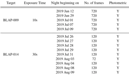
Target Exposure Time Night beginning on No. of frames Photometric BLAP-009 10s 2019 Jun 12 720 Y 2019 Jun 29 720 Y 2019 Jul 01 720 Y 2019 Jul 07 720 Y 2019 Jul 09 720 Y BLAP-014 30s 2019 Jul 26 120 Y 2019 Jul 27 120 Y 2019 Jul 28 120 Y 2019 Jul 29 120 Y 2019 Jul 31 120 Y 2019 Aug 03 72 Y 2019 Aug 04 120 Y 2019 Aug 08 120 Y 2019 Aug 09 120 Y
Table 1.Observation properties for the frames used in the processing of the RISE BLAP-009 and BLAP-014 light curves.
Figure 1.LS periodogram of the RISE light curve of BLAP-009. The
fre-quency spectrum is dominated by the peak at a frefre-quency of 45.091±
0.0138 cycles day−1. This corresponds to a 31.935±0.0098 mins primary pulsation period of the star. The inset focuses on the spectrum between 20−400 cycles day−1revealing the low frequency peaks. The spectral
win-dow function has been over-plotted and shifted to the primary frequency showing the associated sidelobes. Additional peaks are not aligned with the sidelobes and are highlighted by black markers. Their frequencies are shown to be harmonics of the primary frequency in table2and 2 are signif-icantly detected. The horizontal dashed line on both the main plot and the inset denote the 0.01 (1%) significance level. All peaks above this line are considered to be significant.
although it is important to note that this is not due to the precision of the observations and mainly a function of the baseline of the light curve (VanderPlas 2018).
Dashed lines in figures1and2display the 0.01 (1%) signifi-cance level determined using a False Alarm Probability (FAP). This quantity measures the probability that, in the presence of no sig-nal (null hypothesis), a peak of a given size may still result due to a coincidental alignment of Gaussian distributed random errors ( Scar-gle 1982). Making the assumption that the periodogram consists of a number of independent frequencies,Neff, the significant LS power σis calculated using equation2,
σ=−logh1− (1−α)2vn
i
(2)
Figure 2.LS periodogram of the RISE light curve of BLAP-014. The
frequency spectrum is dominated by the peak at a frequency of 42.826±
0.0272 cycles day−1. This corresponds to a 33.625±0.0214 mins primary pulsation period of the star. The inset focuses on the spectrum between 20−
200 cycles day−1revealing the low frequency peaks. The spectral window
function has been over-plotted and shifted to the primary frequency showing the associated sidelobes. There are less additional peaks than BLAP-009 but they also appear to be harmonics of the primary frequency although only 1 is significant. They are highlighted by black markers and shown in table2. The horizontal dashed line on both the main plot and the inset denote the 0.01 (1%) significance level. All peaks above this line are considered to be significant. The peaks are less significant due to the lower number of observations of BLAP-014. This figure has different scales relative to figure1
whereα =0.01 is the significance level,nis the number of
fre-quencies in the frequency spectrum, determined by fmin, fmaxand fstep, andvis the oversampling factor.
We also computed the spectral window functions of the RISE light curves of BLAP-009 and BLAP-014. This calculation is shown in equation3, Pj= 1 N N Õ j=1 exp i2πfjt 2 (3) wherePj is the spectral power of thejth candidate frequency,N
Monoperiodicity of BLAPs
5
is the number of observations in the light curve,iis the imaginary
unit, fj is the jth candidate frequency in the frequency spectrum andtare the time instants of the light curve observations.
This computation is offset to the primary frequency of the two periodograms and over-plotted on the inset plots of figures1 and2. The window function reveals that many of the smaller low frequency peaks for both periodograms are a result of interference from sidelobes in the window function due to the sampling times of the RISE light curves. The signals at these frequencies are aliased from the signal at the primary frequency.
In addition to over-plotting the spectral window function, we also investigated the aliased peaks around the pulsation period from the fine-tuned LS periodograms. These peaks are close to the pri-mary frequency as they are aliased by low frequency sampling periodicity. For BLAP-009, the largest of the peaks surrounding the primary frequency correspond to an alias with a 0.997 day period (1.003 cycles day−1 frequency), the sidereal day. Other peaks are associated with 0.5 and 2 multiples of the sidereal day. The final spurious period causing detectable aliased peaks is approximately 8.2 days (0.122 cycles day−1 frequency). An investigation of this period indicates that it is a result of the schedule of the observa-tion nights. BLAP-014 also shows aliased peaks due to the sidereal day but of weaker power relative to the main pulsation period peak compared with BLAP-009. There also did not appear to be any sig-nificant aliasing from a longer sampling period for this light curve. The periodograms of both BLAP-009 and BLAP-014 do not display any significant high frequency peaks. This indicates the lack of detection of an additional periodic signal. We investigate the limits of this non-detection in the next section. There are a num-ber of additional peaks at lower frequencies once the interference lobes from the spectral window function were identified. Table2 show these frequencies for BLAP-009 and BLAP-014. They are also highlighted in the inset plots of figures1and2by black mark-ers. These peaks are at or near integer multiples of the primary frequency and are associated with higher order harmonics of the primary frequency. This is a result of non-sinusoidal sawtooth sig-nals requiring higher order harmonics to fit the characteristic shape with a set of sinusoids. BLAP-009 displays 3 harmonic frequencies with significant peaks and for BLAP-014 there are 2 significant har-monic frequencies. Determining the significance of these harhar-monic frequencies is important as it determines how many harmonics must be modelled to fit the light curve. The 4thharmonic frequency of BLAP-009 is interesting as it has a smaller peak in the periodogram than the 5thto 8thharmonic frequencies. This is an indication that
the BLAP-009 light curve may contains features which are better modelled by these higher harmonics although their peaks are not sig-nificant. The 3rdharmonic frequency of BLAP-014 also coincides with a sidelobe in the spectral window function which reduces the confidence in this detection.
The light curves for the two BLAPs were then epoch-folded using equation4to reveal the shape of the primary oscillation,
φi(P)=mod
hti−t0
P
i
(4) whereφi(P)is the phase value of the observationias a function of the candidate periodP,tiis the measurement time of the observation
i,t0is an arbitrarily chosen start time (currently defined such as at the
Heliocentric Julian Date (HJD) of 0.0 corresponds to a phase of 0.0),
Pis a candidate period for the light curve and the modulus (mod)
operation retains the decimal component of the calculation (Larsson 1996).
The epoch-folded light curves of BLAP-009 (shown in figure3)
OGLE-BLAP-009
ID Frequency (cycles day−1) Ratio toF
1 Significant F1 45.091 1.000 X F2 90.181 2.000 X F3 134.276 2.978 X F4 178.360 3.956 × F5 227.950 5.056 × F6 273.554 6.067 × F7 314.634 6.978 × F8 359.724 7.978 × OGLE-BLAP-014
ID Frequency (cycles day−1) Ratio toF
1 Significant
F1 42.826 1.000 X
F2 87.660 2.047 X
F3 129.492 3.024 ×
Table 2.Frequencies of harmonic peaks in the periodograms of BLAP-009
and BLAP-014 highlighted by black markers in the inset plots of figures1 and2. The first 3 harmonic frequencies of BLAP-009 and the first 2 harmonic frequencies of BLAP-014 have corresponding periodogram peaks stronger than the 0.01 (1%) significance level.
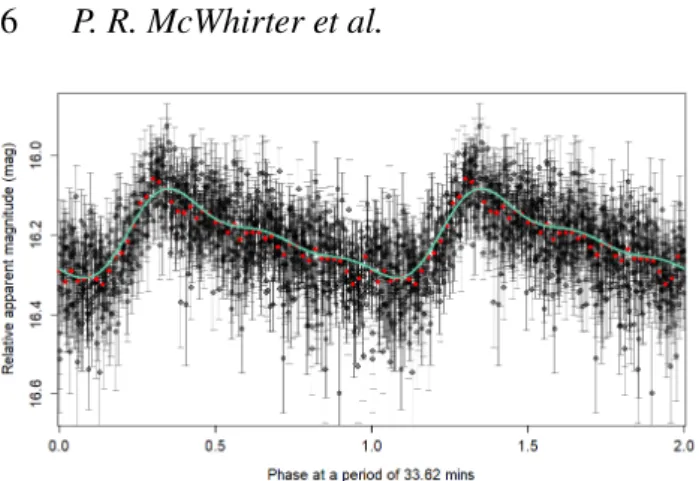
Figure 3.Scatter plot in black shows the folded light curve of BLAP-009 at
a period of 31.935 mins. Weighted average of the light curve with 100 phase bins is shown in red and a fit from a 3-harmonic Fourier model (see table3) is shown in light blue (see online version for colour).
and BLAP-014 (shown in figure4) reveal a characteristic sawtooth shape further reinforcing the conclusion that the additional peri-odogram peaks are harmonics. The epoch-folded light curves were also phase binned into 100 bins using a weighted mean to denoise the light curve further highlighting the oscillation. These binned data points are shown as red diamonds in the figures and the light blue lines are the result of 3-harmonic Fourier fits to the two light curves described in the next section (see online version for colour). BLAP-009 exhibits an interesting and unique feature at maximum light where there appear to be two maxima. This may be a result of one peak corresponding to maximum temperature, and the other for maximum radius. This feature also appears to be present in the OGLE light curves of BLAP-009 but, as of current data, appears to be unique to this BLAP. This may also be the cause for the stronger higher-order harmonic frequency peaks in the BLAP-009 periodogram.
Figure 4.Scatter plot in black shows the folded light curve of BLAP-014 at
a period of 33.625 mins. Weighted average of the light curve with 50 phase bins is shown in red and a fit from a 3-harmonic Fourier model (see table3) is shown in light blue (see online version for colour).
3.2 Search for other signals
To identify further periodic signals in the data, the dominant period in the frequency spectrum must be subtracted out from the light curve in a process namedprewhitening. This is accomplished by fitting a periodic model with the dominant period as the argument. In the case of a sinusoidal signal, a simple sinusoidal model with an amplitude and phase is all that is required. The signals from BLAP-009 and BLAP-014 are clearly non-sinusoidal and appear sawtooth in shape as exhibited by the harmonic peaks in the periodograms; therefore, we select a multi-harmonic Fourier model in order to fit this shape (Deb & Singh 2009;Richards, et al. 2011,2012). The model is shown in Equation5withn=3 as supported by the number
of significant harmonic peaks in the periodogram of BLAP-009,
mi= n Õ j=1 ajsin(2πj f ti)+bjcos(2πj f ti) +b0 (5)
whereb0is the mean magnitude of the light curve,miis the model magnitude of time instantti whereiidentifies theith data point,
aj andbj are Fourier coefficients for the fitted model and f is the dominant frequency, f =P−1wherePis the previously identified
period. This model has 7 coefficients which includes the intercept with an additional 3 sine and 3 cosine components which model the amplitudes and phases of the three sinusoidal harmonics.
Using higher-order harmonics carries an additional risk due to potential over-fitting on noise. To mitigate this, we utilise a regu-larised least-squares fitting technique to apply a weighting to each harmonic proportional to j4wherejis the harmonic number of a
given sinusoid. Equation6is the function to be minimised to find the optimal model,
R(θ, λ)= N Õ i=1 di− θ>ti 2 σ2 i +Nλ n Õ j=1 j4a2j+b2j (6)
whereθis a vector of the model parameters,λis the regularisation parameter,Nis the number of light curve points,di are the photo-metric magnitude data points,ti are the photometric time instants andqa2j+b2jis the amplitude of thejthFourier harmonic andn=3
for the 3-harmonic model. The value of the regularisation parameter allows the control of the smoothing of the model with small values allowing the modelling of high frequency structure and large values smooth this structure out. For these light curves the regularised fit
Coefficient OGLE-BLAP-009 OGLE-BLAP-014
f(cycles/day) 45.0909383371 42.8257928504 c(mag) 15.669736901 16.205144758 a1(mag) 8.3392464×10⁻² −2.7476492×10⁻² b1(mag) 4.7774440×10⁻² 8.1055037×10⁻² a2(mag) −3.7053363×10⁻² 3.4618251×10⁻² b2(mag) −1.7831991×10⁻² 1.7012638×10⁻² a3(mag) 1.0565454×10⁻² 7.773188×10⁻³ b3(mag) 6.159469×10⁻³ −1.7585455×10⁻²
Table 3.Coefficients of regularised 3-harmonic Fourier models of
BLAP-009 and BLAP-014, with periods of 31.935 and 33.625 min respectively. The meanings of these coefficients are shown in equation5.
is applied with a regularisation parameter of 0.01. Table3shows the coefficients of the models fit to the BLAP-009 and BLAP-014 light curves.
This model also allows for the computation of the amplitude of the primary radial amplitude reducing contamination from noise in the observations. Using the coefficients in table3the amplitude of the BLAP-009 pulsation in the RISE 720 nm filter is 0.236 mag. A similar computation using the model of BLAP-014 provides an amplitude of 0.225 mag. These amplitudes are below those reported by P17 from the OGLE I-band light curves which may be a result of noise or the longer wavelengths probed by the RISE 720 nm filter. We also find that our light curves show the oscillations in this band of BLAP-009 are higher amplitude than BLAP-014, disagreeing with the values reported by P17. This discrepancy is likely a result of the difference in the two methods used to determine these values or the differences in the filter bands of OGLE and RISE.
The fitted 3-harmonic Fourier model is then subtracted from the original light curve to leave the prewhitened, residual light curve. We then recomputed the LS periodogram on these resid-uals to search for additional periodic signals shown in figures5and 6. Whilst at first glance, it does appear that BLAP-009 has a sig-nificant low frequency peaks, these were determined to be a result of the sampling cadence by epoch-folding at these frequencies re-vealing extremely poor phase coverage of the resulting folded light curve. Periods over 2 hrs were highly affected by these sampling artifacts. This is an interesting result as each individual night had a 2 hr duration, therefore, this duration is the longest period with a guaranteed complete phase coverage. BLAP-014 also shows a low frequency correlated noise component due to sampling, but it is much less pronounced. The observations for BLAP-014 were over a more regular cadence than BLAP-009 which results in a cleaner power spectrum despite the shorter 1 hr duration of nightly observa-tions. After the explanation of the significant peaks due to correlated noise, the remaining peaks are substantially below the 0.01 (1%) significance level. A few of the larger peaks had their associated frequencies epoch-folded with the prewhitened light curves but no unambiguous signal was found by inspection. Fits of the 3-harmonic Fourier model at these frequencies on the prewhitened data reveal amplitudes of around 10 mmag for BLAP-009 and 40 mmag for BLAP-014 but, despite the regularisation, appear to be fitting noise.
Monoperiodicity of BLAPs
7
Figure 5.LS periodogram of the residual light curve of BLAP-009 after
prewhitening at a period of 31.935 mins. The frequency spectrum is domi-nated by a set of low frequency peaks shown in the inset plot. These peaks were examined and found to be a result of a sampling frequency causing spurious alignment of the data points. The set of peaks near the significance level between 0−500 cycles day−1are higher-order harmonics which were
not prewhitened by the 3-harmonic model. The dashed line denotes the 0.01 (1%) significance level.
Figure 6.LS periodogram of the residual light curve of BLAP-014 after
prewhitening at a period of 33.625 mins. The larger low frequency peak is again associated with a spurious sampling frequency. None of the frequen-cies in the residual spectrum have a significant detection. The dashed line denotes the 0.01 (1%) significance level.
3.3 Null Hypothesis with Artificial Signal Injection
In order to characterise the detection limits of our data as both functions of amplitude and frequency, we inject artificial sinusoidal signal to the data and explore the parameter space in which the signal can be identified with the methodology outlined in §3. A grid of 9×11 period-amplitude pairs were used for the hypothesis
tests of null signals. Any undetected variability is likely to be low amplitude which is usually due to non-radial oscillations which are normally sinusoidal in shape. Due to this, the signals injected into
Figure 7.Contour plot of the normalised LS power interpolated over the
9-amplitude by 11-period grid of sinusoidal signals injected into the RISE light curve of BLAP-009. The green line (see online version for colour) is the contour line denoting the 0.01 (1%) significance level, above which, in the y-axis, the injected signal can be detected.
the data are purely sinusoidal. The LS periodogram may still detect a non-sinusoidal signal but at a lower confidence.
The periods selected for the artificial signals are [2, 5, 10, 20, 30, 60, 120, 300 and 600] mins. The amplitudes of the artificial sinusoids are [1, 2, 5, 10, 15, 20, 25, 30, 40, 50 and 100] mmag. For each combination of period and amplitude, an artificial sinusoidal signal is injected into the light curve and a LS periodogram is computed on the data with a minimum frequency fmin equal to
half of the baseline of the light curve and a maximum frequency
fmax = 900, large enough to include the 2 min periodic signal
with an oversampling factorv=10. The computed period was fit with a 3-harmonic Fourier model and the light curve prewhitened using this model as described in §3. A second LS periodogram is computed on the residual light curve and the LS power of the candidate frequency closest to the period of the artificial signal was calculated along with the significance level.
The contour plots shown in Figures7and8show the results of this analysis for BLAP-009 and BLAP-014 respectively. The con-tours indicate the interpolated LS power across the period-amplitude grid. The light-green line (see online version for colour) indicates the contour of the 0.01 (1%) significance level computed using equation2and is analogous to the dashed lines for the confidence limit in figures1and2. The contours are interpolated across the period-amplitude grid using the Marching Squares algorithm.
The results for BLAP-009 show that any periodic sinusoidal signal can be detected down to a lower threshold than BLAP-014 which is not surprising as BLAP-009 was observed over a longer baseline and with many more individual observations with smaller uncertainties. The strength of the peaks of the pulsation periods was sufficient to not be affected by the injected artificial signal. Therefore, the periods determined by the first LS periodograms were independent of the period and amplitude of the artificial signals. The same cannot be said for the quality of the 3-harmonic Fourier models fit to the pulsation periods. Figure9reveals the magnitude residuals of the fit to the BLAP-009 pulsation period with injected 15.20 mmag sinusoidal signals (the lowest amplitude signal which produces a significant 0.01 (1%) peak in the LS periodogram) for the nine different periods from the grid in Figure7. Despite fitting the same period, the coefficients of the Fourier models differ slightly
Figure 8.Contour plot similar to Figure7for BLAP-014. The green line
(see online version for colour) is the contour line denoting the 0.01 (1%) significance level, above which, in the y-axis, the injected signal can be detected.
Figure 9.Plot of the magnitude residuals of the 3-harmonic Fourier fit to the
BLAP-009 light curve at the pulsation period with an injected 15.20 mmag signal at 9 different periods relative to the observed BLAP-009 light curve. The plot demonstrates that the injected signal can perturb the model fit to the pulsation resulting in unexpected features in Figures7and8. The largest perturbation occurs at periods close to the pulsation period where the amplitude of the residual is 5.94 mmag for a 15.20 mmag signal, a substantial fraction of the injected signal.
due to the effect of the injected signal which results in the residual signal.
The model with an injected signal of period 2 min is almost identical to the initial model and shows the parameters of the Fourier model when unperturbed by the injected signal. The 30 min injected signal residuals show this model is clearly perturbed by the pres-ence of the injected signal as it’s period is similar to the 31.935 min period of the pulsation. The 5.94 mmag amplitude of this residual is a substantial fraction of the injected 15.20 mmag signal. As a result, the Fourier model is under-fitting the pulsation signal and removing some of the injected signal. We conclude that this is the mechanism responsible for the contour feature in Figures7and8 overestimating the LS power of periods close to the pulsation pe-riod of the BLAPs. The 600 min injected pepe-riod light curve model shows a clear variation in the mean magnitude of it’s Fourier fit. This appears to be caused by the sampling of the observations of BLAP-009 as the phase coverage of the light curve decreases above periods of 2 hrs causing inhomogeneous groups of data points when
the light curve is phased at the pulsation period. It is likely that this complication to the Fourier fit, in combination with the poor phase coverage at longer periods producing a correlated noise, results in the unexpected contours in figure7at longer periods where the sig-nificance contour decreases in amplitude until it contacts the zero signal margin. This result suggests that a non-existent signal is sig-nificantly detected which is a nonsensical notion. An inspection of the same feature in the BLAP-014 Fourier fit coefficients reveals this effect is substantially less pronounced for the BLAP-014 light curve reinforced by the lack of contour decay at long periods in Fig-ure8. These features arise as the significance contour is constructed using the FAP which assumes a purely Gaussian noise which does not hold for these light curves.
Taking into account these perturbations, any sinusoidal signal above 15.20±0.26 mmag is significantly detectable to the 0.01 (1%)
significance level in the RISE BLAP-009 light curve. Similarly, any sinusoidal signal above 58.60±3.44 mmag is significantly
de-tectable to the 0.01 (1%) significance level in the RISE BLAP-014 light curve. These boundaries can vary as a function of the period of both the pulsation and the secondary lower-amplitude signal. We can confidently state that our light curves do not show evidence of any additional periodicity given the above confidence limits down to 20 s for BLAP-009 and 60 s for BLAP-014. Additionally, we did not detect any non-significant peak which, when epoch-folded, sug-gested any additional variability. The only detected signals were strongly significant peaks at the two previously identified periods from the OGLE survey.
4 CONCLUSION AND DISCUSSION
This work reports a null multi-periodicity of BLAP-009 down to a 20 s period and BLAP-014 down to a 60 s period with no additional modes with amplitudes greater than 15.20±0.26 mmag for
BLAP-009 and 58.60±3.44 mmag for BLAP-014. The upper limits of the
detectability are heavily influenced by the correlated noise in the light curves produced by the sampling cadence. For BLAP-009 any signal with a period'7 hrs has a peak greater than the 0.01 (1%) significance level. This can be clearly seen in figures5and7. Mean-while, BLAP-014, whilst having a greater limiting amplitude due to less observations has less correlated noise. As a result, we can conclude there are no additional signals up to half of the baseline of the light curve at 6.48 days. Independently, an investigation of the aliased features around the dominant pulsation period and the com-putation of spectral window functions reveal they are all associated with known spurious periods. This work can, however, provide a strong prior in future work in determining the pulsation mode when coupled with multi-band photometry or time-resolved medium/high resolution spectra.
Our data indicate that it is unlikely for there to be additional modes in BLAP-009 and BLAP-014. Radial oscillations in more than one of the fundamental, first or second overtones simultane-ously should be detectable given the computed detection limits of the BLAP-009 light curve. Stellar theory shows that multi-mode pulsators have well-defined period ratios between their fundamen-tal and overtone modes such as P1/P0 = 0.71 for double-mode
Cepheids in the Milky Way (Payne-Gaposchkin & Gaposchkin 1966) andP1/P0 = 0.746 for double-mode RR Lyraes in
glob-ular clusters (Takeuti & Buchler 1993). The structure of BLAPs has not been confidently determined given the likely presence of a de-generate helium core. Despite this, if we assume a similar ratio to the double-mode Cepheids for BLAP-009 and that the detected period
Monoperiodicity of BLAPs
9
is a fundamental mode, the expected periodP1of the first overtone
would be 22.674 mins or a frequency of 63.508 cycles day−1. This frequency should be detectable with our current light curves and is not interfered with by the harmonics of the primary signal. Alterna-tively, if the detected period is the first-overtone, the fundamental mode period is 44.980 mins or a frequency of 32.015 cycles day−1. In this case, the harmonics of the primary signal are also not interfer-ing with the detection of this signal although the window function is much stronger at this frequency for the RISE BLAP-009 light curve. Extrapolating this as common to all BLAPs, the oscillation appears to be a single radial p mode of either the fundamental mode, or the first overtone (Byrne & Jeffery 2018;Paxton, et al. 2019). Other important quantities to refine are the current period of these two BLAPs and the rate of period change relative to the previous OGLE surveys. These values can be used to refine the evolutionary status of these stars as the period of radial pulsation modes is dependent on the mean stellar density (Eddington 1917).
Our precision of the period estimation is lower than the OGLE surveys due to the shorter baseline of the observations as this is the property of the light curve which defines the uncertainty in the frequency spectrum via the Rayleigh frequency resolution:δf =T1,
whereδfis the uncertainty in a frequency measurement andTis the
baseline of the light curve. The larger uncertainties on the periods from the frequency spectra than the OGLE III and IV surveys make it difficult to make conclusions about the rate of period change from our RISE light curves. The faint magnitude of the known candidate BLAPs, even the brightest target BLAP-009, results in substantial difficulty to produce both high cadence light curves with a 2-meter telescope pointing at high air mass whilst maintaining the required signal-to-noise to probe low amplitude oscillations of the order of hundredths of a magnitude.
Future photometric studies on BLAPs would be greatly en-hanced through the identification of additional candidates. Given the null detection of BLAPs in LMC and SMC fields from the OGLE surveys (Pietrukowicz 2018), the Omega-White survey (Macfarlane, et al. 2015) and the ZTF high-cadence survey at low Galactic lati-tudes with ZTF (Bellm, et al. 2019a,b;Graham, et al. 2019) are the most likely ongoing surveys that will yield new BLAPs.
ACKNOWLEDGEMENTS
The Liverpool Telescope is operated on the island of La Palma by Liverpool John Moores University in the Spanish Observatorio del Roque de los Muchachos of the Instituto de Astrofísica de Ca-narias with financial support from the UK Science and Technology Facilities Council.
PRW acknowledges financial support from the Science and Technology Facilities Council (STFC).
ML acknowledges financial support from the OPTICON. PRW thanks the useful discussions with Gavin Ramsay, Si-mon Jeffrey and Conor Byrne from the Armagh Observatory and the recommendations of Alejandra Romero from the Universidade Federal do Rio Grande do Sul.
PRW thanks the comments of the anonymous reviewer con-tributing to the improvement of this manuscript.
REFERENCES
Albrow M. D., et al., 2009, MNRAS, 397, 2099
Albrow M. D., 2017, Pydia: Initial Release On Github. Available at: https://doi.org/10.5281/zenodo.268049
Althaus L. G., Córsico A. H., Isern J., García-Berro E., 2010, A&ARv, 18, 471
Bellm E. C., et al., 2019, PASP, 131, 018002 Bellm E. C., et al., 2019, PASP, 131, 068003 Bramich D. M., et al., 2013, MNRAS, 428, 2275 Byrne C. M., Jeffery C. S., 2018, MNRAS, 481, 3810 Byrne C. M., Jeffery C. S., 2020, MNRAS, 492, 232 Campbell W. W., Wright W. H., 1900, ApJ, 12, 254
Córsico A. H., Althaus L. G., Miller Bertolami M. M., Kepler S. O., 2019, A&ARv, 27, 7
Cox A. N., Morgan S. M., 1989, BAAS, 21, 1095 Deb S., Singh H. P., 2009, A&A, 507, 1729 Deubner F.-L., Gough D., 1984, ARA&A, 22, 593
Dziembowski W. A., Pamiatnykh A. A., 1993, MNRAS, 262, 204 Dziembowski W. A., Moskalik P., Pamyatnykh A. A., 1993, MNRAS, 265,
588
Eddington A. S., 1917, Obs, 40, 290 Eggen O. J., 1952, PASP, 64, 31 Frost E. B., 1902, ApJ, 15, 340
Gautschy A., Saio H., 1995, ARA&A, 33, 75 Gautschy A., Saio H., 1996, ARA&A, 34, 551 Goodricke J., 1786, RSPT, 76, 48
Graham M. J., et al., 2019, PASP, 131, 078001 Green E. M., et al., 2003, ApJL, 583, L31 Jeffery C. S., Saio H., 2006, MNRAS, 371, 659
Kilkenny D., Koen C., O’Donoghue D., Stobie R. S., 1997, MNRAS, 285, 640
Kilkenny D., 2007, CoAst, 150, 234 Kupfer T., et al., 2019, ApJL, 878, L35 Larsson S., 1996, A&AS, 117, 197 Lomb N. R., 1976, Ap&SS, 39, 447
Macfarlane S. A., et al., 2015, MNRAS, 454, 507 Madore B. F., Freedman W. L., 1991, PASP, 103, 933
Paxton B., Bildsten L., Dotter A., Herwig F., Lesaffre P., Timmes F., 2010, MESA: Modules for Experiments in Stellar Astrophysics, ascl:1010.083 Paxton B., et al., 2019, ApJS, 243, 10
Payne-Gaposchkin C., Gaposchkin S., 1966, VA, 8, 191
Pickering E. C., Colson H. R., Fleming W. P., Wells L. D., 1901, ApJ, 13, 226
Pietrukowicz P., et al., 2017, NatAs, 1, 0166 Pietrukowicz P., 2018, pas6.conf, 258, pas6.conf
Pigulski A., Kołaczkowski Z., Ramza T., Narwid A., 2006, MmSAI, 77, 223 Poleski R., et al., 2010, AcA, 60, 1
Ramsay G., 2018, A&A, 620, L9 Richards J. W., et al., 2011, ApJ, 733, 10
Richards J. W., Starr D. L., Miller A. A., Bloom J. S., Butler N. R., Brink H., Crellin-Quick A., 2012, ApJS, 203, 32
Romero A. D., Córsico A. H., Althaus L. G., Pelisoli I., Kepler S. O., 2018, MNRAS, 477, L30
Ruf T., 1999, BRR, 30, 178 Scargle J. D., 1982, ApJ, 263, 835 Shannon C. E., 1949, IEEEP, 37, 10 Smith H. J., 1955, AJ, 60, 179
Smith H. A., 2004, RR Lyrae Stars, Cambridge University Press, Cambridge, UK
Soszynski I., et al., 2008, AcA, 58, 163
Steele I. A., et al., 2004, Proc. SPIE, 679, SPIE.5489 Steele I. A., et al., 2008, Proc. SPIE, 70146J, SPIE.7014 Takeuti M., Buchler J.-R., 1993, Ap&SS, 210
Udalski A., Szymanski M. K., Soszynski I., Poleski R., 2008, AcA, 58, 69 Udalski A., Szymański M. K., Szymański G., 2015, AcA, 65, 1
Unno W., Osaki Y., Ando H., Saio H., Shibahashi H., 1989, Nonradial oscillations of stars, University of Tokyo Press, Tokyo, Japan VanderPlas J. T., 2018, ApJS, 236, 16
Waelkens C., Rufener F., 1985, A&A, 152, 6 Wu T., Li Y., 2018, MNRAS, 478, 3871 MNRAS000,1–10(2020)
Column Description
1 Heliocentric Julian Day (HJD)
2 Phase
3 Relative Photometry / mag 4 Uncertainties / mag
Table A1.The photometry of BLAP-009 and BLAP-014, with periods of
31.935 and 33.625 min respectively. Phase 0.0 is assigned arbitrarily and is defined as phase = 0.0 at HJD = 0.0.
APPENDIX A: RISE PHOTOMETRY
TableA1describes the content of the supplementary material avail-able online for BLAP-009 and BLAP-014.


![[O747.Ebook] Download Ebook Ancient Rhetorics For Contemporary Students.pdf](data:image/gif;base64,R0lGODlhAQABAIAAAP///wAAACH5BAEAAAAALAAAAAABAAEAAAICRAEAOw==)