University of Wisconsin Milwaukee
UWM Digital Commons
Theses and DissertationsDecember 2018
Dynamic Pricing with Variable Order Sizes for a
Model with Constant Demand Elasticity
Nyles Kirk Breecher
University of Wisconsin-Milwaukee
Follow this and additional works at:https://dc.uwm.edu/etd
Part of theMathematics Commons
This Dissertation is brought to you for free and open access by UWM Digital Commons. It has been accepted for inclusion in Theses and Dissertations by an authorized administrator of UWM Digital Commons. For more information, please [email protected].
Recommended Citation
Breecher, Nyles Kirk, "Dynamic Pricing with Variable Order Sizes for a Model with Constant Demand Elasticity" (2018).Theses and Dissertations. 1974.
DYNAMIC PRICING WITH VARIABLE ORDER SIZES
FOR A MODEL WITH CONSTANT DEMAND ELASTICITY
by
Nyles Breecher
A Dissertation Submitted in Partial Fulfillment of the Requirements for the Degree of
Doctor of Philosophy in Mathematics
at
The University of Wisconsin-Milwaukee December 2018
ABSTRACT
DYNAMIC PRICING WITH VARIABLE ORDER SIZES
FOR A MODEL WITH CONSTANT DEMAND ELASTICITY
by Nyles Breecher
The University of Wisconsin-Milwaukee, 2018
Under the Supervision of Professor Richard H. Stockbridge
We investigate a dynamic pricing model under constant demand elasticity which accounts for customers ordering multiple items at once. A closed form expression for the optimal expected revenue and pricing strategy is found. Models with the same demand are shown to have asymptotically similar expected revenue and pricing strategies, even if the order size distributions of the customers are different. Surprisingly, the relative difference between comparable models is shown to be independent of time and the magnitude of demand. Variations of the model are considered, including different low inventory behavior as well as the effect of advertising. Some numerical simulations are presented to provide better insight on the model.
TABLE OF CONTENTS
1 Introduction 1
1.1 Overview . . . 1
1.2 Literature Review . . . 3
1.3 Dynamic Programming Formulation . . . 6
2 Main Results 9 2.1 Analytic Results for the Basic Model . . . 9
2.2 Comparable Models . . . 31
2.3 Numerical Observations . . . 37
3 Extensions 42 3.1 Low Inventory Behavior . . . 43
3.2 Social Efficiency . . . 55
3.3 Advertising and Infinite Time Horizon . . . 58
3.4 Other Arrival Rate Functions . . . 70
4 Conclusion 75
5 Appendix 77
Bibliography 80
LIST OF FIGURES
2.1 Relative difference betweenβn(q)and(n/µ(q)) ε−1
ε and for several order size
distributions q. . . 38 2.2 Relative difference of vn between a variable order model and its comparable
unit order model. . . 39 2.3 Probability distributions of simulated revenue for comparable models while
using policy p∗n(t;q). Per distribution: trials = 20,000, n = 100, T = 30,
ε= 1.5, demand magnitude = 3. . . 40 2.4 Probability distributions of simulated revenue for comparable models with
the same average order size while using policy p∗n(t;q). Per distribution: trials = 100,000, max inventory = 100,T = 30, ε= 1.5, demand rate = 3. . 41 3.1 Expected revenue with λ(p, t) = 2e−2p, T = 5 . . . . 72
3.2 Relative difference between a variable order model compared to unit order model. Solid: λ(p, t) = 2e−2p,T = 5; Dashed: λ(p, t) = 5e−2p. . . . 72
3.3 Expected value with λ(p, t) = 2(2−p) . . . 73 3.4 Relative difference between a variable order model compared to unit order
model. Solid: λ(p, t) = 2(2−p), T = 5; Dashed: λ(p, t) = 5(2−p), T = 5. 74 5.1 Mathematica code which implements basic definitions from the paper. . . . 77 5.2 Mathematica code which implements a Poisson model to simulate the
rev-enue earned while using the optimal pricing strategy. . . 78 5.3 Mathematica code which implements an algorithm to numerically calculate
LIST OF SYMBOLS
p Price. 1
t Current time, note 0≤t≤T. 1
λ(p, t) Customer arrival rate of a Poisson process dependent on price p and current time t. 1
ε Demand elasticity. 1, 9
a(t) Customer arrival rate scaling factor dependent on time t. 1
T Ending time of the sales period. 6
q Probability distribution for the order size of customers. 6
qi Probability that a customer ordersi items, note q= (q1, . . . , qM). 6
M Maximum order size. 6
vn(t;q, λ) Optimal expected revenue with n inventory at current time t for a model with
customer arrival rateλ and customers who have order size distribution q. 6
µ(q) Average order size of the distributionq, µ(q) :=PM
i=1qii. 7
pn(t) A pricing strategy which defines a price at inventory level n at current time t. 7 A(t) Number of future sales at a price equal to 1,A(t) :=RT
t a(s)ds. 10
p∗n(t;q) Price which maximizes expected revenue with n inventory at current time t under order size distribution q. 11
γn(q) The ratio defined as γn(q) := βn(q) nε−ε1
. 15
Mq,λ A Poisson based model where customers have order size distributionqand arrival rate
is λ. 31
gn,t Relative difference between optimal expected revenue of two models. 35
αj Price dependent cost for selling thej-th item (j <0represents overselling costs). 44 rj Price independent cost for selling the j-th item (j <0 represents overselling costs). 44 vC
n(t;q) Optimal expected revenue when customers who want more items than are available
buy all the remaining inventory. 44
m Minimum inventory level. 45
vnG(t;q) Optimal expected revenue when customers who want more items than are available buy no items instead. 45
µC
n(q) Modified average order size for vGn(t;q),µCn(q) :=
PM i=1 qii− Pn j=n−i+1qiαj . 48 µG
n(q) Modified average order size for vnG(t;q), µCn(q) :=
PM∧(n−m) i=1 qii− Pn j=n−i+1qiαj . 48
pCn∗(t;q) Optimal pricing strategy for vnC(t;q). 49
pG∗
n (t;q) Optimal pricing strategy for vnG(t;q). 49
βn(q, B) A β-type sequence with finite sequence B as its base cases. 51 Sn(t;q) Social value. 56
k(t) Represents a tax or subsidy on advertising such that f(t)w is the money spent on advertising which obtains an effective advertising rate w. 58
r(t) Instantaneous discount rate at time t. 59
R(t) Accumulated discount rate, R(t) :=R0δtr(s)ds. 59
vnA Optimal expected revenue when advertising and discounting effects are included. 60
δ Advertising elasticity. 61
γ Joint advertising and demand elasticity,γ := ε1−−1δ. 63
η The term η:= δε δ 1−δ ε−δ ε γ . 63 g(t) The term g(t) :=a(kt)(ft)(δt)ε 1−δ1 . 63 ζ(t) The term ζ(t) :=g(t)ηγ γ−γ1 γ−1 . 63 AAd(t) Defined asAAd(t) :=eγR(t)RtT e−γR(s)g(s)ds. 64 βA
n(q) The β-type sequence which is useful when considering advertising and discounting.
64
MA
q,λ A Poisson based which has arrival rate λ, customer order size distribution q, and
ACKNOWLEDGEMENTS
This research was supported in part by the Simons Foundation (grant award number 246271). We would also like to thank Kurt Helmes for his helpful insights on the asymptotic behavior of βn(q).
1.
Introduction
1.1
Overview
Dynamic pricing concerns sellers who attempt to maximize their profits by adjusting prices over time. The company develops a rule, or pricing strategy, which takes into account market conditions. Take as example the airline industry, where ticket prices are frequently updated based on factors like how much time is left until a flight and how many seats have already been sold. There are many other factors that could influence pricing, although this dissertation focuses on limited time to sell and limited inventory, as these two factors are enough to create interesting models. Some other industries which care deeply about these factors include event ticket sales, fashion, and hotels.
By setting prices, sellers influence the demand for their goods, and more importantly, the amount of revenue they earn. In order to maximize this revenue, a model is needed for sales. Customer arrivals are stochastic and independent of one another, so a Poisson based process is the natural choice for this model. The arrivals are also dependent on the price p and time t. Thus we let λ(p, t) be the intensity of the Poisson based process to reflect these dependencies. We will focus on the case of constant demand elasticity, which necessitates λ(p, t) = a(t)p−ε, where ε is the demand elasticity and a(t) is an arrival rate
scale factor. Demand elasticity is a measure of how much the relative change in quantity demanded changes with respect to a relative change in price. It is an important measure in economics to understand how prices affect sales and helps indicate if items are necessities or luxuries.
Optimal prices are found numerically in many contexts by solving the Hamilton-Jacobi-Bellman (HJB) equations; however, this equation can be difficult to solve in general. The setting of constant demand elasticity offers a tractable example with analytic results, which then lead to deeper insights on the problem itself. This setting has been explored by (McAfee and te Velde 2008) and expanded upon by (Helmes and Schlosser 2013). Compared to these previous works, the key difference for our work is that customers can order multiple items at a time. In terms of the model, that means a compound Poisson process is used instead of a regular Poisson process. To distinguish between these ideas, the compound Poisson setting will be referred to as “variable order sizes,” while the regular Poisson setting will be referred to as “unit order sizes.”
We now outline the structure of this dissertation. Section 1.2 provides a literature review, and highlights papers related to various aspects of our model. Section 1.3 explains the dynamic programming formulation which is used to determine optimal prices. Here, the formulation is presented in a general context and is not tied to constant demand elasticity.
In Chapter 2 we focus on the basic model of constant demand elasticity and variable order sizes, and this section contains the heart of our results. We find closed form expressions for the optimal expected revenue and pricing strategy. A key insight is that this term involved the average order size µ, which is not observed under the unit order case where µ= 1.
In Section 2.2, we turn to comparing constant elasticity models which have the same demand (average rate of sales over time), yet different order size distributions, calling such models comparable. Under constant demand elasticity, we show that as the size of the inventory tends to ∞, comparable models have asymptotically equivalent optimal expected revenue and optimal pricing strategies. This means, that to some degree, unit order models
may be used to approximate variable order models. For low inventory, these differences can be quite large from a revenue management standpoint. Section 2.3 provides numerical results to greater analyze aspects like the convergence rate. We also show the surprising result that the relative difference between comparable models is independent of both time and magnitude of demand; the relative difference is completely determined by the inventory level and the two order size distributions between the comparable models.
Chapter 3 discusses important extensions to the basic problem, which improve the flexi-bility of the model. Section 3.1 discusses the idea of overselling, like an airline overbooking their seats. Determining how to handle low inventory is a problem which must be addressed for variable order sizes, and this section presents a general method for handling these cases. Section 3.2 confirms the result of the unit order case that the monopolist pricing scheme is socially efficient. Section 3.3 introduces advertising and other factors, such as subsidies, into the model. This translates to more involved formulas, but does not fundamentally alter any methods used for the basic model. Lastly, Section 3.4 examines how variable order sizes affect the optimal pricing problem for exponential and linear customer arrival rates.
Lastly, an Appendix includes the Mathematica code which was used in the numerical parts of the dissertation. In particular, functions are provided which can numerically com-pute optimal expected pricing strategies and revenue for any type of customer arrival rate function. These algorithms may be helpful to anyone wishing to do any further work on the subject of variable order sizes.
1.2
Literature Review
Our work is most closely related to that of (McAfee and te Velde 2008) and (Helmes and Schlosser 2013), who both explore the problem of optimal pricing in continuous time with con-stant demand elasticity. (McAfee and te Velde 2008) explored the basic model and (Helmes and Schlosser 2013) expanded on their work by including advertising and other factors like
discounts and subsidies. In both papers, analytic formulas for the optimal pricing strategy are found. These papers also discuss monopolist pricing strategies. With no advertising, a monopolist’s pricing is shown to be efficient, and with advertising a parameter adjustment (like a subsidy) can also ensure this. These papers also show that, in general, waiting as a customer is not a beneficial strategy.
A key feature of these papers and our study is that the specific arrival rate λ(p, t) = a(t)p−ε allows for analytic solutions to be found. Indeed, finding analytic solutions for general λ is difficult primarily because λ may be complicated in general, and even if λ is known, there is not a general analytic solution technique which can be applied in all cases. At the very least, for λ(p, t) = e−p, an analytic solution for the optimal pricing strategy
is shown. This was shown in the seminal paper (Gallego and van Ryzin 1994), which is a widely cited article that created general theory and foundations for dynamic pricing with Poisson models. A wider overview of dynamic pricing models is provided by (Talluri and van Ryzin 2004). This book also contains useful applications of dynamic pricing in the context of specific industries.
The paper by (Monahan, Petruzzi, and Zhao 2004) also considers a dynamic pricing model with constant demand elasticity; however, their model evolves in discrete time. Under the discrete setup, what matters is how many items are sold per time period. This shifts the focus away from customer arrivals, making it significantly different relative to the considerations in our study. (Chung and Flynn 2011) expands upon the discrete time model by introducing holding costs.
At this point we make a note about terminology in the literature. “Demand” is often used interchangeably to refer to the customer arrival rate λ and the rate of sales λµ, where
µ is the average order size. This is not a problem for unit order sizes, where µ = 1 and so demand and the arrival rate are equal; however, it is important to retain this distinction when working with variable order sizes. We have elected to refer to our model as a “variable order size” model to keep the focus on the behavior of customers. Similar generalizations
have been made in other contexts and are sometimes referred to as “batch demand,” “random order rates,” or “compound Poisson demand.” See (Lin, Lu, and Yao 2008), (Elmaghraby and Keskinocak 2008), and (Xu, Yao, and Zheng 2011) for some examples. It is worth noting that in these scenarios when variable order sizes are applied, generally only numerical results are obtained.
Variable order size models also have connections with multiproduct dynamic pricing models. (Gallego and van Ryzin 1997) provides a good reference for this model, and the later paper (Maglaras and Meissner 2006) expands upon their model. Both models consider multiple products which require the same resource. An interesting observation from these papers, although treated briefly, is that a variable order size model can be made equivalent to a multiproduct model by considering each order size level as a different type of product. This similarity is not completely surprising when comparing the optimization equations used: both have a similar form due to a summation term required to handle different types of sales. For the classical models in operations research, the probability distribution of customer order sizes is unaffected by the price. This is a reasonable assumption for industries like airlines or hotels, where a group’s size is essentially fixed before they make a purchase. Therefore, changes in price do not affect the distribution of the number of items purchased. In other scenarios, this assumption may not hold. For example, a particularly good deal on food is likely to induce people to buy more items at a time than they normally would. Discounts for bulk purchasing is also a very common pricing strategy. This practice is called nonlinear pricing, see (Wilson 1993).
The next section shows that low inventory behavior must be addressed to work with a variable order size problem. One approach to handling low inventory is to allow overselling or overbooking. For example, an airline can sell more seats than are actually available on a flight. This is a common practice in the airline industries, as overbooking is a great way for companies to earn extra revenue in spite of cancellations or no sales. Empty spaces on flights essentially represent lost revenue. Of course, overbooking needs to be balanced with the risk
of having too many people for a flight, in which case the airline can offer compensation in the form of upgraded seats or flight discounts. There are many papers which explore the topic of overbooking, see (Kunnumkal and Topaloglu 2009) and (Bertsimas and Popescu 2003) for a couple.
1.3
Dynamic Programming Formulation
We formulate the basic version of the problem. Later, in Chapter 3 we examine extensions. A seller has n items to sell over the time period [0, T], with maximum time 0 < T < ∞. Items have no value after the sales period. The customer arrival rate λ(p, t) is assumed to be known and depends on price p≥0and time 0≤t ≤T. In practice, λ is obtained either from vast amounts of historical data, or more recent data that sellers have gathered. The seller wants to determine the optimal price to use for every time and inventory level which maximizes their total expected revenue. This is known as a pricing strategy.
For now, the specific form ofλ(p, t) is unspecified, as the general model formulation does not depend on the specific λ. Customer arrivals are modeled by a random time change of a compound Poisson process with intensity λ(p, t). Random time change refers to the fact that price p is stochastic in time, as p is set by the seller and will be adjusted based on the specific realization of the process. When a customer arrives, the number of items they order is governed by a probability distribution q = (q1, . . . , qM), where qi, 1 ≤ i ≤ M, is
the probability that the customer orders i items and M is the maximum order size (which can be arbitrarily large, if desired). q is assumed to not depend on price, meaning we are focused on models for industries like airlines and hotels where groups tend to stay together. Let vn(t;q, λ) be the optimal expected revenue with n items to sell, at current time 0 ≤ t ≤ T, under customer order size distribution q and customer arrival function λ. The terms q and λ are after a semicolon to indicate that these features are part of the model setup. Such notation will be useful for comparing models in the future.
The optimal expected revenue has natural boundary conditions: vn(T;q, λ) = 0 (time
for selling is done) andv0(t;q, λ) = 0(no inventory left to sell). One can write a formula for
vn(t;q, λ) by using dynamic programming, also known as the Principle of Optimality. The
principle states that a problem can be divided into several subproblems: at any moment make an optimal choice, and then proceed optimally from that point on.
Formally, let δt > 0 be a small time interval. Since the sales process is Poisson based,
0< i ≤ M items are sold with probabilityqiλ(p, t)δt over the period δt, with a profit of ip
earned. 0 items are sold with probability 1−λ(p, t)δt. In either case, to find an optimal policy, we then proceed optimally with the new inventory and at the new time. Thus the Principle of Optimality states
vn(t;q, λ) = sup p
(1−λ(p, t)δt)vn(t+δt;q, λ)
| {z }
From selling no items
+ M X i=1 qiλ(p, t)δt(ip+vn−i(t+δt;q, λ)) | {z }
From sellingiitems forpeach
. (1.3.1)
Next, we heuristically derive the Hamilton-Jacobi-Bellman equations. More details to val-idate the heuristic derivation of (1.3.2) are provided for more general counting processes in (Bremaud 1981). We rearrange (1.3.1) so that the left hand side is (vn(t +δt;q, λ)− vn(t;q, λ))/δt and then take the limit of the equation as δt→0 to get:
v0n(t;q, λ) =−sup p λ(p, t) " −vn(t;q, λ) + M X i=1 qi(ip+vn−i(t;q, λ)) # . =−sup p λ(p, t) " µ(q)p− vn(t;q, λ)− M X i=1 qivn−i(t;q, λ) !# , (1.3.2) whereµ(q) :=PM
i=1qiiis the average order size of the order size distributionq. The Principle
of Optimality states that a pricing policy pn(t) which satisfies the supremum in (1.3.2) for
The recursive elements in (1.3.1) and (1.3.2) show that M base case terms of vn are
needed for these equations to be well defined. The simplest choice is to definevn(t;q, λ) = 0
for n < 0. Under this assumption, (1.3.1) models overselling with no penalty costs, since items can be sold to go into negative inventory. The practice of overselling actually common in the airline industry, where some passengers are expected to miss their flights. Of course, there is a risk to do so, as a plane might be overfull and compensation needs to be given out. Without penalty costs, the current behavior of the model may feel a bit limited. We note that the results in Chapter 2 are primarily recursive in nature, so the behavior at low inventory often plays an unimportant role, as the eventually recursion drives the results. This will formally be explored in Section 3.1. So for now we will assumevn(q;q, λ) = 0when n <0 for ease of exposition.
2.
Main Results
In this chapter, constant demand elasticityεis now assumed. As will be shown, this property requires that λ(p, t) = a(t)p−ε. This chapter has three parts. Section 2.1 proves a closed
form solution for the optimal expected revenue. Its asymptotic behavior is then analyzed, the results of which are used in Section 2.2, which focuses on comparable models. These are models with the same demand, but different order size distributions. Comparable models are found to have the same asymptotic behavior in the inventory size. A surprising result is that the relative difference between comparable models does not depend on time or the magnitude of demand. Finally, Section 2.3 shows some numerical calculations in order to obtain a better understanding of the model as a whole.
2.1
Analytic Results for the Basic Model
Demand Qis the rate of item sales, which is calculated by multiplying the rate of customer arrivals λ(p, t) by a customer’s average order size µ, that is Q(p, t) := λ(p, t)µ(q). Demand elasticityεmeasures how sensitive that demand is to price fluctuations. εis a measure of the relative change in demand compared the relative change in price, taken in absolute value, thus ε:= dQ/Q dp/p =−p(dQ/dp) Q =− p(dλ/dp) λ . (2.1.1)
Note that the evaluation of the absolute value is justified because for all practical purposes, quantity demanded and price are inversely proportional, making(dQ/Q)/(dp/p)≤0. Since constantεis assumed, (2.1.1) can be solved forλthrough separation of variables. This yields
λ(p, t) = a(t)p−ε for some time-dependent function a(t)>0, which is an arrival rate scaling
factor. An interesting feature of this arrival rate λ form is that it can be made arbitrarily large by takingp→0, thus ensuring all inventory can always be sold.
For this chapter, λ is always of the forma(t)p−ε, so write vn(t;q) = vn(t;q, λ)for clarity.
Substituting λ(p, t) =a(t)p−ε into (1.3.2) yields
vn0(t;q) = −sup p a(t)p−ε " −vn(t;q) + M X i=1 qi(ip+vn−i(t;q)) # =−sup p a(t)p−ε " µ(q)p− vn(t;q)− M X i=1 qivn−i(t;q) !# . (2.1.2)
Using standard calculus, the price p∗ which attains the supremum in (2.1.2) is found to be
p∗n(t;q) = ε ε−1µ(q) −1 vn(t;q)− M X i=1 qivn−i(t;q) ! . (2.1.3)
An immediate consequence of this formula is thatε >1, since the solutions forε≤1 would make no practical sense. From an economic standpoint this also makes sense, since goods with ε ≤ 1 are not considered elastic goods. That means that price has little influence on their demand, meaning that dynamic pricing is of little use. With pricing strategy (2.1.3),
v0n(t;q) =−a(t)µ(q)ε(ε−1) ε−1 εε vn(t;q)− M X i=1 qivn−i(t;q) !1−ε . (2.1.4)
Before proceeding, some notation is needed. Their meaning and usefulness will become more apparent through the proofs. Let A(t) := RtT a(s)ds, which can be thought of as the expected number of future customer arrivals at a price of 1. Also let(βn(q))nbe the sequence
given by βn(q) = 0 for n≤0 and such that for n >0, βn(q) is the non-negative solution to ε−1 ε =βn(q) 1 ε−1 βn(q)− M X i=1 qiβn−i(q) ! . (2.1.5)
Equation (2.1.5) will be helpful because it mirrors some structure in (2.1.4). Note that analytically finding βn(q) would be cumbersome if not impossible, but can be computed
numerically rather simply. The existence and uniqueness of a solution to (2.1.5) is given by the following lemma:
Lemma 2.1.1. Let fb,c(x) :=x 1 ε−1 (bx−c) =bx ε ε−1 −cx 1
ε−1 for any constants b >0 and c.
Then there exists a unique positive solution to fb,c(x) = ε−ε1.
Proof. Let b > 0 and c be constants. Then fb,c(x) < 0 for 0 < x < c/b, fb,c(x) = 0 at x = c/b, and fb,c(x) > 0 and increasing for x > c/b. Therefore fb,c(x) = ε−ε1 has a unique
positive solution.
The lemma applies to (2.1.5) because when computing βn+1(q), all previous βi(q) for i < n+ 1 are known. Therefore we can think of (2.1.5) as the equation ε−ε1 =fb,c(βn+1(q)),
where b = 1 and c = PM
i=1qiβn−i(q). The lemma is simple, but will be a useful reference
in Section 3.1, where new types of sequences like βn(q) are examined. Now we present the
optimal pricing policy.
Theorem 2.1.2. With arrival rateλ(p, t) = a(t)p−ε and customer order sizesq, the optimal
expected revenue is
vn(t;q) = µ(q)βn(q)A(t)1/ε. (2.1.6)
Furthermore, the optimal pricing strategy is
p∗n(t;q) =βn(q)−1/(ε−1)A(t)1/ε.
Proof. Proceed by induction to show (2.1.6) holds. Forn ≤0, by definition, βn(q) = 0 and vn(t;q) = 0, showing that (2.1.6) holds. Recall Equation (2.1.4),
vn0+1(t;q) = −a(t)µ(q)ε(ε−1) ε−1 εε vn+1(t;q)− M X i=1 qivn+1−i(t;q)) !1−ε . (2.1.7)
This is an ordinary differential equation, so verifying that the induction hypothesis holds for this equation will complete the induction. Note that throughout this proof t and q
dependencies are often suppressed for readability. Assume Equation (2.1.6) holds up to n. Then (2.1.7) becomes vn0+1 =−aµε(ε−1) ε−1 εε vn+1− M X i=1 qiµβn+1−iA1/ε !1−ε . (2.1.8)
To prove that the induction assumption holds for n + 1, we substitute the induction as-sumption for n+ 1 into (2.1.8) and show that the equality remains true. Substituting the induction assumption for n+ 1 into the left-hand side of (2.1.8) yields
vn0+1 =µβn+1 1 εA (1/ε)−1dA dt =−aµ ε A (1−ε)/ε βn+1.
Substituting the induction assumption (2.1.6) into the right-hand side of (2.1.8) gives
−aµε(ε−1) ε−1 εε µβn+1A 1/ε− M X i=1 qiµβn+1−iA1/ε !1−ε =−aµ(ε−1) ε−1 εε A (1−ε)/ε β n+1− M X i=1 qiβn+1−i !1−ε =−aµA(1−ε)/ε1 ε ε−1 ε ε−1 βn+1− M X i=1 qiβn+1−i !1−ε =−aµ ε A (1−ε)/ε βn+1,
where the last equality is justified by the definition of βn(q), equation (2.1.5). This shows
that the left- and right-hand sides of (2.1.8) are equal for the induction assumption atn+ 1, thus verifying the equation
vn(t;q) = µ(q)βn(q)A(t)1/ε
holds for all n. Furthermore, by substituting that equation into (2.1.3) gives
p∗n(t;q) = ε ε−1µ(q) −1 µ(q)β n(q)A(t)1/ε− M X i=1 qiµ(q)βn−i(q)A(t)1/ε ! =A(t)1/ε ε ε−1 βn(q)− M X i=1 qiβn−i(q) ! =A(t)1/ε ε−1 ε ε−1 βn(q)− M X i=1 qiβn−i(q) !1−ε −1/(ε−1) =A(t)1/εβn(q)−1/(ε−1),
finishing the proof.
Equation (2.1.6) reveals the term µ(q), which was not observed for the unit order case shown in (McAfee and te Velde 2008), where µ = 1. The equation appears to match our intuition that as the average order sizeµ(q)increases, so does our optimal expected revenue; however, it is important to note that as qchanges, so does βn(q). Therefore, more analysis
of βn(q) is necessary to truly understand (2.1.6).
Lemma 2.1.3. βn(q) is a non-decreasing sequence in n.
Proof. For n ≤ 0, βn(q) = 0. Proceed by induction and assume βk−1(q) ≤ βk(q) for all k < n−1. Recall (2.1.5), the recursion equation for βn(q):
ε−1 ε =βn(q) 1 ε−1 β n(q)− M X i=1 qiβn−i(q) ! ,
or multiplied out as ε−1 ε =βn(q) ε ε−1 − M X i=1 qiβn−i(q)βn(q) 1 ε−1. (2.1.9)
Solving for βn(q) happens recursively. So in solving (2.1.5) for βn(q), it is assumed for any i < n thatβi(q)would be known. Thus we treat the right hand side of (2.1.9) as a function
of the variable βn(q). That is, we can think of the function
f(x) = xε−ε1 − M X i=1 qiβn−i(q)x 1 ε−1,
where finding x > 0 such that ε−ε1 = f(x) is equivalent to solving for βn(q). Similarly,
writing g(x) =xε−ε1 − M X i=1 qiβ(n−1)−i(q)x 1 ε−1
and solving for x > 0 such that ε−ε1 = g(x) would give the value of βn−1(q). Lemma 2.1.1
shows that the positive solutions for ε−ε1 =f(x) and ε−ε1 =g(x) exist and are unique. Next we show the solution to ε−ε1 = f(x) is greater than or equal to the solution of
ε−1
ε = g(x). Compare the coefficients of f(x) and g(x). The induction hypothesis shows
that the coefficients of f(x) are less than or equal to those in g(x). Therefore, for positive
x, f(x)≤ g(x). Thus the positive solution to f(x) = ε−ε1 must be greater than or equal to the positive solution to g(x) = ε−ε1, or equivalently, βn(q) ≥ βn−1(q). This completes the
induction proof, proving that βn(q) is a non-decreasing sequence inn.
This lemma confirms the intuition that the optimal expected revenue vn(t;q) should
increase as the inventory n increases. For an example why βn(q) is not always strictly
increasing, consider the order size distribution q = (0,1). That is, customers buy 1 item with probability 0 and 2 items with probability 1. In this case, the recursion equation (2.1.5) is the same for n = 1 and n = 2, β1(q) = β2(q). The lack of a strictly increasing property
for βn(q) is one of the reasons that analysis of βn(q) is more difficult for variable orders
The next step is to look at βn(q) as n → ∞. As it turns out, βn(q) is asymptotically
equivalent to nε−ε1, up to a scale factor based on µ(q). So we define γn(q) = βn(q) nε−ε1
to help simplify notation. For the unit order case,γn(q)has monotonicity and a simple upper bound
which makes finding its limit relatively straightforward. Unfortunately, when generalizing to variable order sizes, these properties are not true for all q and so the proof of the limiting behavior of γn(q) is more difficult. Before finding lim
n→∞γn(q), several lemmas are needed to
help identify the asymptotic behavior of γn(q).
The first lemma contains a function whose recursive structure is similar to that ofβn(q).
The asymptotic properties of this function are therefore useful in examining the asymptotic properties of βn(q).
Lemma 2.1.4. The function
f(n;q) := n 1− M X i=1 qi n−i n ε−ε1!
is decreasing for n > M, n ∈R. Moreover,
lim n→∞f(n;q) =µ(q) ε−1 ε .
Proof. Letn > M, n ∈R. First we show that f has a limiting value: lim n→∞f(n;q) = limn→∞ 1−PM i=1qi n−i n ε−ε1 1/n H = lim n→∞ −PM i=1qi ε−ε1 n−i n −1/ε i n2 −1/n2 = lim n→∞ M X i=1 iqi ε−1 ε n−i n −1/ε = M X i=1 iqi ε−1 ε =µ(q) ε−1 ε
Note that f is continuous for n > M, so if f is concave up (f00 > 0), then f must decrease to the limit value just shown. In other words, to show that f is decreasing for n > M, we will show that it is concave up. Start with f0, which is
f0(n;q) =n − M X i=1 qi ε−1 ε n−i n −1/ε i n2 ! + 1− M X i=1 qi n−i n ε−ε1! =1− M X i=1 qi ε−1 ε n−i n −1/ε i n + n−i n ε−ε1! =1− M X i=1 qi n−i n −1/ε iε−i nε + n−i n =1− M X i=1 qi n n−i 1/ε 1− i nε .
Then f00(n;q) =− M X i=1 qi " n n−i 1/ε i n2ε + 1 ε n n−i 1ε−1 −i (n−i)2 nε−i nε # =− M X i=1 iqi ε n n−i 1/ε" 1 n2 − n n−i −1 1 (n−i)2 nε−i nε # =− M X i=1 iqi εn2 n n−i 1/ε 1− nε−i nε−iε >0.
Note that the inequality is justified since ε > 1 implies that 1− nε−i nε−iε
< 0. Thus f is concave up, completing the proof of Lemma 2.1.4.
The next lemma gives conditional bounds for γn(q), based on properties γn(q) might
satisfy. These properties involve checking whether γn(q) is the minimum or maximum of
itself and the previous M terms in the γn sequence. It seems that, numerically, γn(q)
satisfies the given properties for large enough inventory n. That said, there are challenges with proving this analytically for any q. Fortunately, the proof of lim
n→∞γn(q) in Theorem
2.1.7 will sidestep this issue by considering all cases for γn(q), whether the term meets has
the given properties or not.
Lemma 2.1.5. (a) lim inf
n→∞ γn(q)>0.
(b) If there exists a strictly increasing sequence (Nk)k⊂N such that γNk(q) = min
0≤i≤MγNk−i(q) for all k, then lim infn→∞ γn(q)≥µ(q) 1−ε
ε .
(c) If there exists an N ≥M such that γN(q) = max
0≤i≤MγN−i(q), then lim sup n→∞ γn(q)≤µ(q) 1−ε ε .
Proof. Proof of part (a): Recall γn(q) = βn(q)/n ε−1
ε . By definition, βn(q) ≥ 0, and
therefore γn(q) ≥ 0 and lim inf
n→∞ γn(q) ≥ 0. Assume to the contrary that lim infn→∞ γn(q) = 0.
and the subsequence contains all γNk(q) such that γNk(q) = min
1≤i≤Nk
γi(q). In other words,
the subsequence contains all terms γn which are the smallest value seen up to that term.
This also gives that lim
k→∞γNk(q) = 0.
Let δ > 0. Then there exists a k > 0 such that γNk(q) ≤ δ. Substitute γNk(q)N ε−1
ε
k =
βNk(q) into (2.1.5), noting that the inequality is justified by the construction of γNk(q),
ε−1 ε =γNk(q) 1 ε−1N k γNk(q)− M X i=1 qiγNk−i(q) Nk−i Nk ε−ε1! ≤γNk(q) 1 ε−1N k γNk(q)− M X i=1 qiγNk(q) Nk−i Nk ε−ε1! (2.1.10) =γNk(q) ε ε−1N k 1− M X i=1 qi Nk−i Nk ε−ε1! =:γNk(q) ε ε−1f(N k;q) (2.1.11)
By Lemma 2.1.4, f(n;q) is decreasing for n > M and therefore f(Nk;q)≤ f(M;q). Thus
from (2.1.11) we get ε−1 ε ≤γNk(q) ε ε−1f(M;q)≤δ ε ε−1f(M;q),
but this is a contradiction since f(M;q) is a constant while δ is arbitrary. Therefore
lim inf
n→∞ γn(q)6= 0, completing the proof of part (a).
Proof of part (b): Suppose there exists an increasing sequence(Nk)ksuch thatN1 > M
and γNk(q) = min
0≤i≤MγNk−i(q) for all k. Assume that (Nk)k contains every integer n > M
such that γn(q) = min
0≤i≤Mγn−i(q). First we get a bound for lim infk→∞ γNk(q), then we show
lim inf
k→∞ γNk(q) = lim infn→∞ γn(q).
Note that γNk(q) = min
thus (2.1.11) holds for all k as well: ε−1 ε ≤γNk(q) ε ε−1f(N k;q),
or written another way,
γNk(q)≥ ε−1 εf(Nk;q) ε−ε1 .
Let δ > 0. By Lemma 2.1.4, there exists a K ≥ M such that for all k ≥ K, f(Nk;q) ≤ µ(q) ε−ε1(1 +δ) and thus γNk(q)≥ 1 µ(q)(1 +δ) ε−ε1 . Therefore lim inf k→∞ γNk(q)≥lim infk→∞ 1 µ(q)(1 +δ) ε−ε1 = 1 µ(q)(1 +δ) ε−ε1 ,
but δ was arbitrary and so
lim inf k→∞ γNk(q)≥ 1 µ(q) ε−ε1 =µ(q)1−εε .
With a bound established, we now show that lim inf
k→∞ γNk(q) = lim infn→∞ γn(q).
For each j ≥N1, defineaj such thatNaj ≤j < Naj+1. We claim that
γj(q)≥γNaj(q). (2.1.12)
To prove the claim, consider if j = Naj. Then γj(q) = γNaj(q) and the claim is true. If j > Naj, suppose towards contradiction that γj(q) ≤ γNaj(q). Without loss of generality
assume thatj is the smallest value greater thanNaj such thatγj(q)≤γNaj(q)holds. If not,
we could just find some value between Naj and j which is. Then γj(q) = min
min
0≤i≤Mγj−i(q), and so j ∈ (Nj)j. But also (Nj)j is an increasing sequence and j > Naj, so j ≥Naj+1. This contradicts the fact thatNaj ≤j < Naj+1. Hence γj(q)≥γNaj(q), proving
claim (2.1.12). This equation then shows
lim inf
j→∞ γj(q)≥lim infj→∞ γNaj(q).
Also (Nj)j is a subsequence of (Naj)j, and thus lim inf
j→∞ γNaj(q)≥ lim infj→∞ γNj(q). Combining
everything together yields
lim inf
j→∞ γj(q)≥lim infj→∞ γNaj(q)≥lim infj→∞ γNj(q)≥µ(q) 1−ε
ε ,
completing the proof of part (b).
Proof of part (c) Assume there exists an N1 such that N1 > M and γN1(q) = max
0≤i≤MγN1−i(q). We follow the same development in part (a) for equation (2.1.11), except
our assumption now reverses inequality (2.1.10), thus
ε−1
ε ≥γN1(q) ε ε−1f(N
1;q).
Use the fact from Lemma 2.1.4 that f is decreasing and lim
n→∞f(n;q) = µ(q) ε−1 ε to get ε−1 ε ≥γN1(q) ε ε−1µ(q) ε−1 ε , or µ(q)1−εε ≥γN1(q).
Now suppose N2 is the smallest value greater thanN1 such thatγN2(q)> µ(q) 1−ε
ε . Then γN2(q) = max
N1−M≤i≤N2γi(q) = max0≤i≤MγN2−i(q). But by the same argument for N1, µ(q) 1−ε
ε ≥
γN1(q), a contradiction. Hence no such N2 exists and γn(q) ≤ µ(q) 1−ε
ε for all n > N1,
The next lemma relates lim supγn(q)and lim infγn(q). These relations are helpful with
the conditional bounds from Lemma 2.1.5, as we will be able to obtain equalities instead of inequalities. This proof is the most involved proof of the dissertation, and illustrates how variable order sizes can complicate the basic problem. In this case, the complication comes from not being able to prove that γn(q) actually has specific properties for alln.
Lemma 2.1.6. (a) 1 lim sup n→∞ γn(q) 1 ε−1 ≤µ(q) lim inf n→∞ γn(q). (b) 1 lim inf n→∞ γn(q) 1 ε−1 ≥µ(q) lim sup n→∞ γn(q).
Proof. Proof of part (a) The idea of this proof is to start with the recursive equation for βn(q) in (2.1.5). From there we significantly alter the look of the equation in order to
write it using the successive difference terms ∆βn(q) :=βn(q)−βn−1(q). These successive
differences will prove to be useful due to the fact that they have a convenient bound which we now show. Since the qi form a probability distribution,PMi=1qi = 1 and thus
∆βn(q) = βn(q)−βn−1(q) =βn(q)− M X
i=1
qiβn−1(q).
Lemma 2.1.3 states that βn(q) is non-decreasing in n, thus from the previous equation we
get ∆βn(q)≤βn(q)− M X i=1 qiβn−i(q).
for βn(q), equation (2.1.5). Thus we can substitute to get ∆βn(q)≤ ε−1 ε 1 βn(q)1/(ε−1) , (2.1.13)
giving a bound for ∆βn(q). Differences between non-successive βn(q) can be written as a
telescoping sum of successive differences, that isβn(q)−βn−k(q) = Pk −1
j=0∆βn−j(q). This fact
is also useful for finding bounds. We now reformulate (2.1.5) by using successive differences. Recall also that the average order size is given by µ(q) =PM
i=1iqi. Equation (2.1.5) is now reformulated: ε−1 ε 1 βn(q) 1 ε−1 =βn(q)− M X i=1 qiβn−i(q) = M X i=1 qi(βn(q)−βn−i(q)) = M X i=1 i−1 X j=0 qi∆βn−j(q) = M X i=1 qi " ∆βn(q) + i−1 X j=1 ∆βn−j(q) # = M X i=1 qi∆βn(q) + M X i=1 i−1 X j=1 qi∆βn−j(q) = M X i=1 iqi∆βn(q)− M X i=1 (i−1)qi∆βn(q) + M X i=1 i−1 X j=1 qi∆βn−j(q) =µ(q)∆βn(q)− M X i=1 i−1 X j=1 qi∆βn(q) + M X i=1 i−1 X j=1 qi∆βn−j(q) =µ(q)∆βn(q)− M X i=1 i−1 X j=1 qi[∆βn(q)−∆βn−j(q)] Substitute βn(q) =n ε−1
ε γn(q) into the left hand side of the previous equation to get
ε−1 ε 1 n1εγn(q) 1 ε−1 =µ(q)∆βn(q)− M X i=1 i−1 X j=1 qi[∆βn(q)−∆βn−j(q)]. (2.1.14)
It may look odd to have both γn(q) and β terms in the equation. Eventually (2.1.13) will
be used to eliminate any β terms from the equation, while keeping only the one γn(q)term.
Let δ >0. Then choose Nδ large enough such that for all n≥Nδ.
1 γn(q) 1 ε−1 ≥ 1 lim sup k→∞ γk(q) 1 ε−1 −δ (2.1.15)
We now explain why such an Nδ exists. First note that Lemma 2.1.5(a) states that lim inf
n→∞ γn(q)>0, and so the right hand side of (2.1.15) is not ∞. Then Nδ can be chosen
large enough to ensure that whenever γn(q) > lim sup k→∞
γk(q), that γn(q) is close enough lim sup
k→∞
γk(q)in order to satisfy (2.1.15). Wheneverγn(q)≤lim sup k→∞
γk(q), (2.1.15) is already
satisfied.
LetN > Nδ. Eventually we will take the limit asN → ∞, but for now we sum equation
(2.1.14) from n=Nδ toN to obtain N X n=Nδ ε−1 ε 1 n1εγn(q) 1 ε−1 = N X n=Nδ µ(q)∆βn(q)− N X n=Nδ M X i=1 i−1 X j=1 qi[∆βn(q)−∆βn−j(q)].
Note the telescoping sum
N P n=Nδ
∆βn(q) =βN(q)−βNδ−1(q), making the previous equation
N X n=Nδ ε−1 ε 1 n1εγn(q) 1 ε−1 =µ(q)(βN(q)−βNδ−1(q))−S, (2.1.16)
where the telescoping sum also is used for writing
S = M X i=1 i−1 X j=1 qi[(βN(q)−βNδ−1(q))−(βN−j(q)−βNδ−j−1(q))].
Why is this new form useful? Note that ∆βN(q) =βN(q)−βN−1(q) depends on the N for
two terms. However, the telescoped sum
N P n=Nδ
∆βn(q) =βN(q)−βNδ−1(q) only depends on N for one term. So asN → ∞, βNδ−1(q)remains fixed while βN(q) increases.
Next we eliminate the summation on the left-hand side of (2.1.16). Observe the the following sum can be thought of as a Riemann sum estimate of an integral, that is,
N X n=Nδ 1 n1ε ≥ Z N+1 Nδ x−1/εdx≥ Z N Nδ x−1/εdx= ε ε−1 Nε−ε1 −N ε−1 ε δ .
Applying the previous inequality along with (2.1.15) to equation (2.1.16) yields
Nε−ε1 −N ε−1 ε δ 1 lim sup n→∞ γn(q) 1 ε−1 −δ ≤µ(q)(βN(q)−βNδ−1(q))−S, and dividing by Nε−ε1, 1− Nδ N ε−ε1! 1 lim sup n→∞ γn(q) 1 ε−1 −δ ≤µ(q) γN(q)− βNδ−1(q) Nε−ε1 − S Nε−ε1 .
Now take the liminf as N → ∞ to get
1 lim sup n→∞ γn(q) 1 ε−1 −δ≤lim inf N→∞ µ(q)γN(q)− S Nε−ε1 . (2.1.17)
In order to simplify the liminf further, we now show that lim
N→∞ S Nε−ε1 = 0. Begin by writing S= M X i=1 i−1 X j=1 qi[[βN(q)−βNδ−1(q)]−[βN−j(q)−βNδ−j−1(q)]] = M X i=1 i−1 X j=1 qi[[βN(q)−βN−j(q)]−[βNδ−1(q)−βNδ−j−1(q)]] = M X i=1 i−1 X j=1 qi "j−1 X k=0 ∆βN−k(q)−[βNδ−1(q)−βNδ−j−1(q)] # . (2.1.18) Then S Nε−ε1 ≤ M X i=1 i−1 X j=1 qi "j−1 X k=0 ∆βN−k(q) Nε−ε1 + βNδ−1(q)−βNδ−j−1(q) Nε−ε1 #
Using this inequality along with with the bound (2.1.13) yields S Nε−ε1 ≤ M X i=1 i−1 X j=1 qi "j−1 X k=0 ε−1 ε 1 βN−k(q)1/(ε−1)N ε−1 ε + βNδ−1(q)−βNδ−j−1(q) Nε−ε1 #
Then since Nδ is fixed, the right hand side of this inequality goes to 0 as N → ∞ (recall
that Lemma 2.1.3 stated thatβn(q) was non-decreasing in n). Therefore
0 = lim N→∞ S Nε−ε1 . Thus (2.1.17) becomes 1 lim sup n→∞ γn(q) 1 ε−1 −δ≤µ(q) lim inf N→∞ γN(q). (2.1.19)
Since this equation is true for all δ >0, we get
1 lim sup n→∞ γn(q) 1 ε−1 ≤µ(q) lim inf n→∞ γn(q), (2.1.20)
completing the proof of part (a).
Proof of part (b) The proof of part (b) is done in a nearly identical way to part (a). The adjustments are mostly in notation: limsup is exchanged with liminf, the inequalities are reversed, and a +δ is needed instead of −δ. For instance, the analog of (2.1.15) is
1 γn(q) 1 ε−1 ≤ 1 lim inf n→∞ γn(q) 1 ε−1 +δ. (2.1.21)
To summarize these lemmas, Lemma 2.1.5 gives conditional bounds forγn(q)and Lemma
2.1.6 gives useful relations relating lim infγn(q) to lim supγn(q). We now use these results
Theorem 2.1.7. For any choice of ε >1 and order size distribution q, lim n→∞γn(q) = limn→∞ βn(q) nε−ε1 =µ(q)1−εε .
Proof. Suppose the following claim is true (it will be proved later in the proof):
lim sup n→∞
γn(q) = lim inf
n→∞ γn(q) = limn→∞γn(q). (2.1.22)
Then substituting this equation into Lemma 2.1.6(a) and Lemma 2.1.6(b) gives
1 lim n→∞γn(q) 1 ε−1 ≤µ(q) lim n→∞γn(q) 1 lim n→∞γn(q) 1 ε−1 ≥µ(q) lim n→∞γn(q),
meaning equality holds,
1 lim n→∞γn(q) 1 ε−1 =µ(q) lim n→∞γn(q).
Solving for the limit gives
lim
n→∞γn(q) =µ(q) 1−ε
ε ,
which proves the theorem.
Now we prove the claim. This is accomplished by considering three cases, based on whether the following properties hold or not:
Property 1: There exists an infinite, increasing sequence (Nk)k ⊂ N such that γNk(q) = min
0≤i≤MγNk−i(q) for all k.
Property 2: There exists an N ≥M such thatγN(q) = max
0≤i≤MγN−i(q).
Proof of claim, case 1: Suppose Property 1 holds. Then the conditions of Lemma 2.1.5(b) are met and thus
lim inf
n→∞ γn(q)≥µ(q) 1−ε
ε .
Combining this with inequality from Lemma 2.1.6(b) gives
1 (µ(q)1−εε ) 1 ε−1 ≥ 1 lim inf n→∞ γn(q) 1 ε−1 ≥µ(q) lim sup n→∞ γn(q),
and simplifying µ(q) terms yields
µ(q)1−εε ≥lim sup n→∞ γn(q). Therefore µ(q)1−εε ≥lim sup n→∞ γn(q)≥lim inf n→∞ γn(q)≥µ(q) 1−ε ε ,
and equality holds throughout, proving claim (2.1.22) for case 1.
Proof of claim, case 2: Suppose Property 2 holds. Then by Lemma 2.1.5(c), lim sup n→∞ γn(q)≤µ(q) 1−ε ε .
Combining this with Lemma 2.1.6(a) we get
1 (µ(q)1−εε ) 1 ε−1 ≤ 1 lim sup n→∞ γn(q) 1 ε−1 ≤µ(q) lim inf n→∞ γn(q),
and simplifying the µ(q) terms yields
µ(q)1−εε ≤lim inf
Therefore
µ(q)1−εε ≤lim inf
n→∞ γn(q)≤lim supn→∞ γn(q)≤µ(q) 1−ε
ε ,
and equality holds throughout, proving the claim for case 2.
Proof of claim, case 3: Suppose neither Properties 1 nor 2 hold. The idea of this case is to find a sequence of upper and lower bounds for γn(q), then to show that the difference
between these upper and lower bound sequences goes to 0.
Since Property 1 is false, there exists an N1 > M such that for all n ≥ N1, γn(q) 6= min
0≤i≤Mγn−i(q). Let (Nk)k ⊂ N be a strictly increasing sequence starting with N1 such that
for all k the condition
γNk−M(q) = min
0≤i≤MγNk−i(q) (2.1.23)
holds. That is, γNk−M(q)is the minimum of itself and the next M terms in the γ sequence.
Why does such a sequence exist? Suppose instead (Nk)k ⊂ N is any strictly increasing
sequence starting with N1. We can use this sequence to construct one which also satisfies
(2.1.23). Let 0 < lk ≤ M be such that γNk−lk(q) = min
0≤i≤MγNk−i(q). In other words, lk
is the value of i which achieves the minimum min
0≤i≤MγNk−i(q). If lk = M, then condition
(2.1.23) holds for Nk. Note that lk 6= 0 since for all n > N1, γn(q) 6= min
0≤i≤Mγn−i(q). By
the same reasoning, γNk+1(q) 6= min
0≤i≤MγNk+1−i(q), and thus γNk−lk(q) = min0≤i≤MγNk+1−i(q).
Repeat this argument to see γNk−lk(q) = min
0≤i≤MγNk+(M−lk)−i(q), or written another way, γ(Nk+M−lk)−M(q) = min
0≤i≤Mγ(Nk+M−lk)−i(q). This shows condition (2.1.23) holds for Nk + M −lk. Therefore the sequence (Nk+M −lk)k satisfies condition (2.1.23) for all k. Lastly, (Nk+M−lk)k may not be strictly increasing, but sinceNk is strictly increasing andM−lk ≥ 0, a strictly increasing subsequence of(Nk+M−lk)kexists, thereby showing the appropriate
sequence exists.
We now aim to find lower and upper bounds for γn(q). For all k ≥1, let ak =Nk−M.
Thenγak(q) = min
0≤i≤MγNk−i(q)by the properties of(Nk)k. Suppose somenis the firstn > ak
such that γn(q) < γak(q). Then γn(q) = min Nk−M≤i≤n
γi(q) = min
contradiction since all γn(q) for n > N1 lack this property. Therefore there is no n > ak
such that γn(q)< γak(q), giving for all k the lower bound
γak(q)≤lim inf
n→∞ γn(q). (2.1.24)
For all k ≥ 1, let bk be such that Nk −M < bk ≤ Nk and γbk(q) = max
0≤i≤MγNk−i(q)
(note that bk 6= Nk−M = ak, because γak(q) = min
0≤i≤MγNk−i(q)). Suppose n is the first n > bk such that γn(q) > γbk(q). Then γn(q) = max
Nk−M≤i≤n
γi(q) = max
0≤i≤Mγn−i(q). But
this is a contradiction since Property 2 is false. Therefore there is no n > bk such that γn(q)> γbk(q), giving the upper bound for all k
lim sup n→∞
γn(q)≤γbk(q). (2.1.25)
Equations (2.1.24) and (2.1.25) together imply that
lim sup n→∞
γn(q)−lim inf
n→∞ γn(q)≤γbk(q)−γak(q). (2.1.26)
Thus a bound for γbk(q)−γak(q) is also a bound forlim sup n→∞
γn(q)−lim inf
n→∞ γn(q).
To help towards finding a bound, recall equation (2.1.13) of Lemma 2.1.6:
βn(q)−βn−1(q)≤ ε−1 ε 1 βn(q)1/(ε−1) . (2.1.27)
Thus the following is true (notes have been added to the left-hand side in the calculation to provide specific justification for some steps):
γbk(q)−γak(q) = βbk(q) b ε−1 ε k − βak(q) a ε−1 ε k (ak < bk by construction)≤ βbk(q) b ε−1 ε k − βak(q) b ε−1 ε k
= 1 b ε−1 ε k (βbk(q)−βak(q)) = 1 b ε−1 ε k bk X i=ak+1 βi(q)−βi−1(q) (Equation (2.1.27))≤ 1 b ε−1 ε k bk X i=ak+1 ε−1 ε 1 βi(q)1/(ε−1)
(Lemma 2.1.3 statesβn(q) is non-decreasing)≤ 1 b ε−1 ε k bk X i=ak+1 ε−1 ε 1 βak+1(q) 1/(ε−1) (bk−ak≤M by construction, ε−1 ε <1)≤ 1 b ε−1 ε k M βak+1(q) 1/(ε−1) . (2.1.28)
Now combining (2.1.26) and (2.1.28) we get, for each k,
lim sup n→∞ γn(q)−lim inf n→∞ γn(q)≤γbk(q)−γak(q)≤ 1 b ε−1 ε k M βak+1(q) 1/(ε−1) . (2.1.29)
Note that bk is a sequence of increasing integers, since Nk−M < bk ≤ Nk and Nk was an
increasing sequence of integers. Also, βk(q) is at worst non-decreasing in k. So taking the
limit of (2.1.29) as k → ∞ shows that
0≤lim sup n→∞ γn(q)−lim inf n→∞ γn(q)≤0, or in other words, lim sup n→∞ γn(q) = lim inf n→∞ γn(q) = limn→∞γn(q),
proving the claim for case 3.
It is quite surprising that βn(q) has such a simple comparison in the limit, given that
(2.1.5), the recursion equation for βn(q), looks quite complex. Theorem 2.1.7 shows again
the importance of the average order size term µ(q), which is not observed in the unit order case where µ(q) = 1. The term µ(q) was also seen in Theorem 2.1.2, which said that the optimal expected revenue was given byvn(t;q) =µ(q)βn(q)A(t)1/ε.
The limit in Theorem 2.1.2 along with the formula for vn(t;q) imply the intuitive result
that, since ε−ε1 < 1, having more inventory has diminishing returns. Also consider from Theorem 2.1.2 the formula for the optimal price, p∗n(t;q) = βn(q)−1/(ε−1)A(t)1/ε. The limit
of Theorem 2.1.2 shows that p∗ changes less and less as n → ∞. This is in line with the idea that dynamic pricing becomes less relevant with large inventory, and will have the best benefits for small to moderate inventory.
From a practical or numerical standpoint, the simpler term (n/µ(q))ε−ε1 can be used
to approximate βn(q), and therefore vn(t;q) = µ(q)βn(q)A(t)1/ε ≈ n ε−1
ε (µ(q)A(t)) 1
ε. This
approximation can be important to save computation time if n is very large or there are a lot of order sizes. However, as the next section will show, there is very useful application of the approximation when looking at comparable models.
2.2
Comparable Models
We now turn to the analysis of comparable models, that is, models which have the same demand yet have different order size distributions. Let Mq,λ denote a model with order size
distribution qand arrival rate λ(p, t). Define two models Mq,λ and Mq¯,¯λ to be comparable
if their demands are equal for all p >0 and 0< t < T, i.e.
λ(p, t)µ(q) = ¯λ(p, t)µ(¯q).
For constant demand elasticity, arrival rates are of the form λ(p, t) = a(t)p−ε and λ¯(p, t) = ¯
a(t)p−ε. Thus we see an equivalent condition to (2.2) is
a(t)µ(q) = ¯a(t)µ(¯q). (2.2.1)
An important observation from (2.2.1) is that the arrival rate scaling factor ¯a(t) is just a scalar multiple of a(t). Observe that if Mq,λ and Mq¯,λ¯ are comparable, then so are Mq,cλ
and Mq¯,cλ¯ for any constant c > 0. Thus, to help distinguish between these types of cases,
it is helpful to think about the term a(t)µ(q) as a demand rate scaling factor (or demand magnitude), similar to howa(t)is the arrival rate scaling factor. The second theorem in this chapter will examine sets of comparable models which have the same order size distributions, but different demand magnitudes.
Since we are now considering how multiple models compare,λcan no longer be suppressed in notation for terms like vn. For example, vn(t;q, λ) is the optimal expected revenue and p∗n(t;q, λ) is the optimal pricing strategy for a model with order size distribution q and customer arrival rate λ. The next result shows some interesting asymptotic behavior of the optimal expected revenue and price for comparable models.
Theorem 2.2.1. LetMq,λ andM¯q,λ¯ be comparable models which both have constant demand
elasticity ε. Then, lim n→∞ vn(t;q, λ) vn(t; ¯q,λ¯) = 1 and lim n→∞ p∗n(t;q, λ) p∗ n(t; ¯q,λ¯) = 1.
In other words, Mq,λ and M¯q,¯λ have asymptotically equivalent optimal expected revenue and
pricing strategies.
Proof. LetMq,λandM¯q,λ¯be comparable models withλ(p, t) =a(t)p−εandλ¯(p, t) = ¯a(t)p−ε.
Recall Theorem 2.1.2 which stated that vn(t;q) = µ(q)βn(q)A(t)1/ε. This was for a model
with λ(p, t) =a(t)p−ε but now λ dependencies mater, so the notation of the formula must
be updated. Define A(t;a) = RtT a(s)ds and A(t; ¯a) =RtT ¯a(s)ds. Then Theorem 2.1.2 says
vn(t;q, λ) = µ(q)βn(q)A(t;a)1/ε. (2.2.2)
Also recall Theorem 2.1.7, which stated lim n→∞
βn(q) nε−ε1
= µ(q)1−εε . Let δ > 0. By combining
(2.2.2) with Theorem 2.1.7 we see that there exists Na >0 such that for all n > Na, vn(t;q, λ)−µ(q) n µ(q) ε−ε1 A(t;a)1ε < δ.
Similarly, there existsNa¯ >0such that for all n > N¯a, vn(t; ¯q,λ¯)−µ(¯q) n µ(¯q) ε−ε1 A(t; ¯a)1ε < δ.
Note that for a constantc,A(t;ca) =RtT ca(t)dt=cRtT a(t)dt =cA(t;a). We also have from the condition for comparable models (2.2.1) thata(t) = ¯a(µt)(µq(¯)q). Thus
µ(q) n µ(q) ε−ε1 A(t;a)1ε =µ(q) n µ(q) ε−ε1 A t;¯aµ(¯q) µ(q) 1ε =µ(q) n µ(q) ε−ε1 µ(¯q) µ(q) 1ε A(t; ¯a)1ε =µ(¯q) n µ(¯q) ε−ε1 A(t; ¯a)1ε.
Then for n >max(Na, N¯a),
vn(t;q, λ)−vn(t; ¯q,λ¯) ≤ vn(t;q, λ)−µ(q) n µ(q) ε−ε1 A(t;a)1ε + µ(¯q) n µ(¯q) ε−ε1 A(t; ¯a)1ε −v n(t; ¯q,λ¯) <2δ.
Sinceδwas arbitrary, this proves that two comparable models have asymptotically equiv-alent optimal expected revenues as n → ∞.
Theorem 2.1.2 also gives the optimal expected revenue asp∗n(t;q) = βn(q)−1/(ε−1)A(t)1/ε.
2.1.7 there exists an N such that for all n > N, p∗n(t;q, λ)− n µ(q) ε−ε1!− 1 ε−1 A(t;a)1ε = p∗n(t;q, λ)− n µ(q) −1ε A(t;a)1ε < δ p∗n(t; ¯q,¯λ)− n µ(¯q) ε−ε1!− 1 ε−1 A(t; ¯a)1ε = p∗n(t; ¯q,¯λ)− n µ(¯q) −1ε A(t; ¯a)1ε < δ. Also, n µ(q) −1ε A(t;a)1ε = n µ(q) −1ε µ(¯q) µ(q) 1ε A(t; ¯a)1ε = n µ(¯q) −1ε A(t; ¯a)1ε Therefore p∗n(t;q, λ)−pn∗(t; ¯q,λ¯)≤ p∗n(t;q, λ)− n µ(q) −ε1 A(t;a)1ε + n µ(¯q) −ε1 A(t; ¯a)1ε −p∗ n(t; ¯q,¯λ) <2δ
Hence the optimal pricing strategies for the comparable models are asymptotically equivalent as n→ ∞.
Observe that given a particular model Mq,λ, we can always find a comparable model Mq¯,¯λ of any order size distribution q¯. Comparable models have equal demands, that is λ(p, t)µ(q) = ¯λ(p, t)µ(¯q). So set λ¯(p, t) = µ(q)/µ(¯q)λ(p, t) in order to makeMq,λ and M¯q,¯λ
comparable. In particular, by choosing q¯ = (1), a variable order size model always has a comparable unit order size model.
Theorem 2.2.1 proves the intuitive idea that models where inventory is being sold at similar rates will have similar behavior. The next natural question to ask is how similar are comparable models? One measure of the difference between two comparable models is
their relative difference. Define the relative difference of optimal expected revenue between comparable models Mq,λ and Mq¯,¯λ by
gn,t(Mq,λ,Mq¯,λ¯) :=
vn(t;q, λ)−vn(t; ¯q,λ¯) vn(t; ¯q,¯λ)
,
for 0≤t < T and n >0.
Theorem 2.2.2. LetMq,λ andM¯q,λ¯ be comparable models which both have constant demand
elasticity ε. For any 0≤t < T and n >0,
gn,t(Mq,λ,M¯qλ¯) = µ(q) µ(¯q) (ε−1)/ε βn(q)−βn(¯q) βn(¯q) .
Notably, the relative difference g does not depend on time nor the demand magnitude of the models.
Proof. LetMq,λandM¯q,λ¯be comparable models withλ(p, t) =a(t)p−εandλ¯(p, t) = ¯a(t)p−ε.
Since the models are comparable, (2.2.1) holds and so a(t) = a¯(µt)(µq(¯)q). Recall the optimal expected revenue from Theorem 2.1.2, modified to include all relevant dependencies,
vn(t;q, λ) = µ(q)βn(q)A(t;a)1/ε.
gn,t(Mq,λ,Mq¯,¯λ) = vn t;q,λµ¯µ((¯qq))−vn(t; ¯q,¯λ) vn(t; ¯q,¯λ) = µ(q)βn(q) At;¯aµµ((¯qq)) 1/ε −µ(¯q)βn(¯q)A(t; ¯a)1/ε µ(¯q)βn(¯q)A(t; ¯a)1/ε = µ(q)βn(q) µ(¯q) µ(q) 1/ε A(t; ¯a)1/ε−µ(¯q)β n(¯q)A(t; ¯a)1/ε µ(¯q)βn(¯q)A(t; ¯a)1/ε = µ(q) µ(¯q) (ε−1)/ε βn(q)−βn(¯q) βn(¯q) .
Consider two comparable models and then consider those models with their demand mag-nitudea(t)µ(q)doubled. For the demand magnitute expression,µ(q)does not change in this scenario, doubling demand magnitude is equivalent to doubling a(t). Theorem 2.2.2 states that their relative difference will not change. This is surprising, since it might intuitively feel like increased demand should lead to increased differences between the models. The key feature which enables the proof of Theorem 2.2.2 is that the formula for the optimal expected revenue is separable. This property allows the time terms a(t) and ¯a(t) to drop out. Since demand magnitude is given by a(t)µ(q), but in this scenario µ(q) is fixed, changing the demand magnitude equates to changing a(t). Thus changing the demand magnitude does not change the relative difference.
One of the main goals of this dissertation is to identify the changes generated by gen-eralizing unit order models to variable order models. In the previous section, we saw how analytic results changed and the new techniques needed to handle these changes. This sec-tion provided a structure that can be used to compare models and presented results related to these ideas. Of particular note is that variable order models have a comparable model which only has unit orders. In the next section we will use numerical observations to get a
more concrete idea of what variable order size models look like, especially relative to their unit order counterparts.
2.3
Numerical Observations
This section will provide graphs from numerical calculations to help visualize the results proven thus far in the dissertation. Note that many of the graphs will show continuous plots even though the graphs are technically discrete plots. This makes the graphs easier to parse. Additionally, all of the the code used in this section is presented in the appendix.
We begin with Theorem 2.1.7, which stated that
lim
n→∞γn(q) = limn→∞ βn(q)
nε−ε1
=µ(q)1−εε .
One of the crucial observations from this result is that
n µ(q)
ε−ε1
is an approximation for
βn(q), a fact seen in Theorem 2.2.1. In a practical context, such an approximation would
be useful in the case where βn(q) may be slow to compute. Such might be the case if
dynamic prices are needed frequently. Thus having an idea of how quickly βn(q) converges
toµ(nq)
ε−1 ε
is useful.
An algorithm in Mathematica was created to numerically calculateβn(q). Figure 2.1 uses
the algorithm to compute βn(q) and then compare convergence of βn(q) and (n/µ(q)) ε−1
ε
for four different order size distributions. Note that for these distributions, full weight was not put on qM because then the graph shows multiple lines per distribution and is hard to
interpret. This is due to βn(q)only changing every M terms if qM = 1.
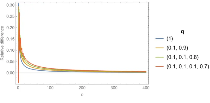
Models with larger µ(q) appear to have slower convergence rates. We observe from the graph that order size distributions with larger µ(q) converge more slowly. That said, convergence is within 1% by n = 250, even for the distribution with the highest µ. This appears like relatively quick convergence considering large aircraft can easily carry over 500 passengers and concert venues often have thousands of seats.
Figure 2.1: Relative difference between βn(q) and (n/µ(q)) ε−1
ε and for several order size
distributions q. 0 100 200 300 400 0.00 0.05 0.10 0.15 0.20 0.25 0.30 n Relative difference q (1) (0.1, 0.9) (0.1, 0.1, 0.8) (0.1, 0.1, 0.1, 0.7)
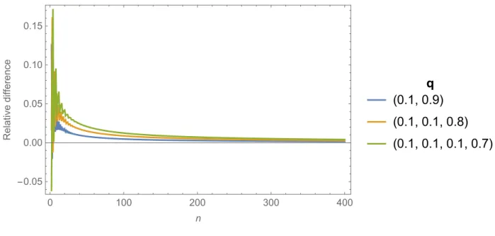
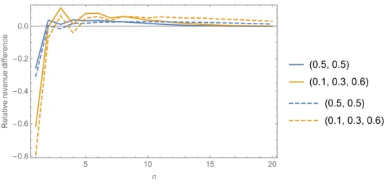
Figure 2.2 shows similarly quick convergence for the optimal expected revenue for a variable order model to its comparable unit order model. This is an important comparison to consider because it indicates the numerical differences between variable order and unit order models. Again, larger average order sizes lead to slower convergence. In this graph we observe that there appears to be more noise for low inventory. This is due to overselling, which allows variable order models to have higher potential revenue at low inventory. Once the inventory size gets large enough, this benefit is largely mitigated. This is one of the reasons why we have waited to address alternative low inventory behavior until Section 3.1.
Figure 2.2: Relative difference ofvn between a variable order model and its comparable unit order model. 0 100 200 300 400 -0.05 0.00 0.05 0.10 0.15 n Relative difference q (0.1, 0.9) (0.1, 0.1, 0.8) (0.1, 0.1, 0.1, 0.7)
Now we consider more general comparable models. The main result for comparable models is Theorem 2.2.1, which states that the expected total revenue of comparable models have the same asymptotic behavior in the inventory n. Figure 2.2 gave one application of this idea by comparing the optimal expected revenue of variable order and unit order models. But there is more to consider than just the expected value. Since the model is a compound Poisson type process, any realization of the model will involve randomness.
To examine this randomness, a Mathematica program was created to simulate the Poisson based process defined in section 1.3. One property of Poisson processes with intensity λ is that over a small interval of timeδtthere is aλδtchance of a customer arriving. By choosing a specific value forδt the problem is discretized, which allows the digital implementation of the model. That said, based on testing different δt, the discretization does not need to be super fine to obtain precise results. We choose δt to be around 0.2% of the total time scale for our results.
In each time step, the program randomly determines if a customer arrives, based on the arrival rate λ(p, t). Any pricing policy can be used to then update λ(p, t) for the next time
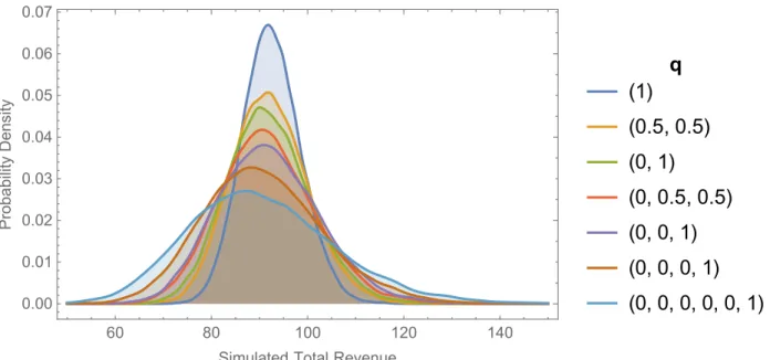
step. At the end of the simulation, the amount of money earned from sales is recorded. Figure 2.3 shows probability distributions of this simulated revenue. To generate each distribution, 20,000 trials were run. Each density curve corresponds to a model which uses a different order size distribution q; however, all models used are comparable with demand magnitude 3. The figure confirms the intuition that as the average order size increases, so does the variance of the revenue.
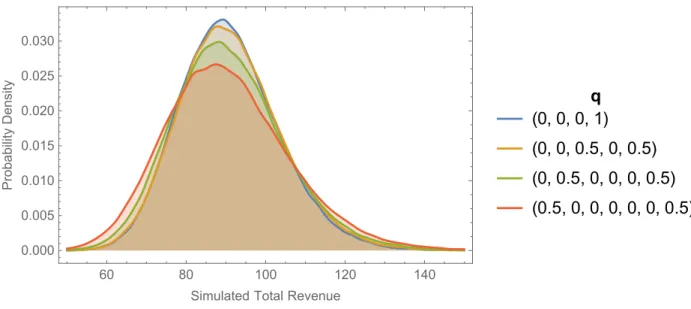
Quantifying the exact amount of variance for each density curve is tricky though. For one, the expected revenue can never go below 0, giving a 1 sided lower limit. But also, multiple order size distributions can have the same average order size. This idea is explored in Figure 2.4, which shows several comparable models which have the same µ(q), but different order size distributions. Note that these models presented in that plot are all comparable to the models used in Figure 2.3 too. Figure 2.4 reveals that the maximum order size also plays a role in how spread the simulated revenue is.
Figure 2.3: Probability distributions of simulated revenue for comparable models while using policy p∗n(t;q). Per distribution: trials = 20,000, n = 100, T = 30, ε = 1.5, demand magnitude = 3. 60 80 100 120 140 0.00 0.01 0.02 0.03 0.04 0.05 0.06 0.07
Simulated Total Revenue
Probability Density q (1) (0.5, 0.5) (0, 1) (0, 0.5, 0.5) (0, 0, 1) (0, 0, 0, 1) (0, 0, 0, 0, 0, 1)
Figure 2.4: Probability distributions of simulated revenue for comparable models with the same average order size while using policy p∗n(t;q). Per distribution: trials = 100,000, max inventory = 100, T = 30, ε= 1.5, demand rate = 3.
60 80 100 120 140 0.000 0.005 0.010 0.015 0.020 0.025 0.030
Simulated Total Revenue
Probability Density q (0, 0, 0, 1) (0, 0, 0.5, 0, 0.5) (0, 0.5, 0, 0, 0, 0.5) (0.5, 0, 0, 0, 0, 0, 0.5)
The observations in this section highlight interesting aspects of our problem, and the fig-ures provide a more concrete context through which the model can be understood. Analytic results can inform the numerical results, and vice versa. So understanding both gives better understanding of the model. In fact, the numerical algorithms were the original indicator for the comparison results in Section 2.3. We hope that the programs used in this section and presented in the appendix are useful to anyone who wishes to do any future work regarding the variable order size model.