Geometry of random 3-manifolds
Dissertation zur
Erlangung des Doktorgrades (Dr. rer. nat.) der
Mathematisch-Naturwissenshaftlichen Fakult¨at der
Rheinischen Friedrich-Wilhelms-Universit¨at Bonn
vorgelegt von
Gabriele Viaggi
aus
Carrara, Italien
Fakult¨at der Rheinischen Friedrich-Wilhelm-Universit¨at Bonn
1 Gutachter: Prof. Dr. Ursula Hamenst¨adt 2 Gutachter: Prof. Dr. Sebastian Hensel Tag der Promotion: 24 Januar 2020 Erscheinungsjahr: 2020
SUMMARY
We studyrandom 3-manifolds, as introduced by Dunfield and Thurston, from a geometric point of view. Within this framework, work of Maher allows us to equip a typical random 3-manifold with a canonical geometric structure, namely, ahyperbolic metric.
By Mostow rigidity, such metric is unique up to isometries and, hence, we can attach to a random 3-manifold geometric invariants such as volume, Laplace and length spectra, diameter.
Our goal is to develop tools to compute these invariants and, in general, to get an effective and explicit description of the hyperbolic structure. More precisely, in this thesis we obtain the following results:
(1) We compute thecoarse growthrate of volume, diameter and spectral gap for a typical family of random 3-manifolds.
(2) We show that the volumes of random 3-manifolds obey to a law of large numbers.
(3) We find an explicit model manifold that captures, up to uniform bilipschitz distortion, the geometry of a random 3-manifold.
Contents
1. Introduction 9
2. Small eigenvalues of random 3-manifolds 23
3. Volumes of random 3-manifolds 73
INTRODUCTION
Geometry of random 3-manifolds
The purpose of this work is to study random 3-manifolds, as introduced by Dunfield and Thurston [15], from a geometric point of view1.
The notion of random 3-manifold that we use comes from the obser-vation that certain families of closed orientable 3-manifolds are naturally parametrized by diffeomorphisms of surfaces. We consider two examples: Heegaard splittingsand fibered 3-manifolds.
The first family consists of those 3-manifoldsM with a Heegaard decom-position of genusg ≥2. This means that M is diffeomorphic a 3-manifold Mf obtained by gluing together two copies of a handlebody Hg of genus g
along a diffeomorphismf of their boundaries∂Hg = Σ
Mf :=Hg∪f:∂Hg→∂Hg Hg.
The second example is the family of 3-manifoldsM that fiber over the circle with a fiber Σ of genus g ≥ 2. In this case, M is diffeomorphic to the mapping torusTf of a diffeomorphism f of the fiber Σ
Tf := Σ×[0,1]/(x,0)∼(f(x),1).
The diffeomorphism type of the 3-manifoldsMf andTf only depends on the
isotopy class off, which means that it is well-defined for themapping class [f]∈Mod (Σ) := Diff+(Σ)/Diff0(Σ) in themapping class group.
Following [15], we define a family of random Heegaard splittings, or ran-dom 3-manifolds, as one of the form (Mfn)n∈N where (fn)n∈N is a random walk on the mapping class group driven by some initial probability measure µwhose support is finite and generates Mod(Σ). We denote by Pn the
dis-tribution of the n-th step of the walk fn and by P the distribution of the
sample path (fn)n∈N.
Analogously, we can define families of random mapping tori (Tfn)n∈N. The reason for comparing mapping tori and Heegaard splittings is that, geometrically, they behave similarly in random families as we will see.
We focus now on random Heegaard splittings.
The original approach to random 3-manifolds by Dunfield and Thurston was mostly topological and group theoretic. However, in their foundational paper [15], they also considered the geometric side and made the following
1A list of references is provided at the end of each of the four parts of the thesis. The references for the introduction are on page 21.
Conjecture (Dunfield-Thurston, Conjecture 2.11 in [15]). A random 3-manifold is hyperbolic and its volume grows linearly in the step of the walk. We remark that the problem of finding hyperbolic structures on most Heegaard splitting of a fixed genusg≥2 was originally raised by Thurston (see Problem 24 in [31]). The introduction of the notion of random 3-manifolds allows to make the statement of the problem more precise.
After Perelman’s solution of Thurston’s geometrization conjecture, the only obstruction to the existence of a hyperbolic metric on Mf can be
phrased in topological terms: A closed orientable 3-manifold is hyperbolic if and only if it is irreducible and atoroidal. Mapping classes that are suf-ficiently complicated in an appropriate sense (see Hempel [17]) give rise to Heegaard splittings that satisfy these properties.
Relying on this criterion, Maher established the existence of a hyperbolic metric on random 3-manifolds
Theorem (Maher [22]). A random 3-manifold is hyperbolic.
This is the starting point for our work. By Mostow rigidity, such a metric is unique up to isometry, thus it makes sense to refine Dunfield and Thurston question and study the growth of geometric invariants, such as volume, diameter, length spectrum and eigenvalues of the Laplacian in families of random 3-manifolds.
We will work towards this goal and develop a moreconstructiveand effec-tiveapproach to the hyperbolization of random 3-manifolds. In particular, we give an answer to Dunfield and Thurston’s conjecture interpreting it in a strict way.
We state informally our contribution
Theorem 1. There is an explicit, Ricci flow free, hyperbolization for ran-dom 3-manifolds. Furthermore, the volumes of ranran-dom 3-manifolds obey to a law of large numbers.
We will formulate precise statements for the two parts of Theorem 1 only later on (as Theorems 10 and 4).
By explicit Ricci flow free hyperbolization we mean that we construct the hyperbolic metric by assembling simple pieces and that we only use tools from the deformation theory of Kleinian groups. We use the model manifold technology by Minsky [25] and Brock, Canary and Minsky [10], as well as the effective version of Thurston’s Hyperbolic Dehn Surgery by Hodgson and Kerckhoff [18] and Brock and Bromberg’s Drilling Theorem [8].
We remark that, even though we do not rely on Perelman’s geometriza-tion, we do use the main result from Maher [22], namely, the fact that the Hempel distanceof the Heegaard splittings (see [17]) grows coarsely linearly along the random walk.
Our construction gives new and more refined information than the mere existence of a hyperbolic metric. In fact, we also provide a model mani-foldthat captures, up to uniform bilipschitz distorsion, the geometry of the random 3-manifold and allows the computation of its geometric invariants. The additional structure that we get is the one of a -model metric. We describe it in the next pargraph.
A model metric. The existence of a hyperbolic metric does not guarantee by itself much control on the invariants of a random 3-manifold such as volume, Laplace and length spectra or diameter.
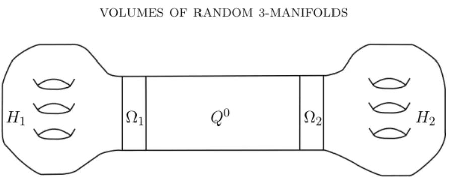
Following a strategy started by Minsky, Namazi, Brock and Souto [25], [26], [27], [12], we first construct a much more controlled negatively curved metric (Mf, ρ) which we can handle explicitly and then use it to understand
the underlying hyperbolic structure. The requirements we want to impose are the following: There exists < 1/2 such that (Mf, ρ) decomposes into
five piecesMf =H1∪Ω1∪Q∪Ω2∪H2 satisfying
(1) Topologically,H1 andH2are homeomorphic to genusghandlebodies while Ω1,Ω2 and Qare homeomorphic to Σ×[1,2].
(2) Geometrically, ρ has negative curvature sec∈(−1−,−1 +), but outside the region Ω = Ω1∪Ω2 the metric is purely hyperbolic. (3) Volume-wise, we have vol(Q)≥(1−)vol(M).
(4) The piece Q is almost isometrically embeddable in a complete hy-perbolic 3-manifold diffeomorphic to Σ×R.
We call such a metric a-model metric.
The importance of the last requirement resides in the fact that we un-derstand explicitly hyperbolic 3-manifolds diffeomorphic to Σ×Rthanks to the work of Minsky [25] and Brock, Canary and Minsky [10] which provides a detailed combinatorial description of their internal geometry.
Our first result, which is joint work with Ursula Hamenst¨adt, is the fol-lowing:
Theorem 2. For every 0< <1/2 we have
Pn[Mf admits a-model metric]n−→→∞1.
Observe that Theorem 2 does not immediately provide an explicit relation between the-model metric and the underlying hyperbolic structure. How-ever, the presence of a-model metric gives a lot of mileage on the topology and geometry of the 3-manifold as we will explain in a moment.
Before going on, we should mention that, using a result claimed by Tian [32], the mere fact that a metricρ is a -model metric and that the region Ω where it is not hyperbolic has uniformly bounded diameter (as follows from the proof of Theorem 2), implies, if >0 is sufficiently small, that ρ is uniformly close up to third derivatives to a hyperbolic metric. However, Tian’s result is not published and we do not rely on it.
Volumes of random 3-manifolds. Our strategy for the computation of the geometric invariants given the data of a -model metric is simple to explain. We first compute the invariant for the middle piece Q using the model manifold technology [25], [10]. Then, we argue that the invariant of Qis uniformly comparable to the one of Mf in a random setting.
The first example we provide is a computation of the volume growth rate. It is an immediate consequence of our construction, work of Besson, Courtois and Gallot [4], and work of Brock [7].
Proposition 3. There exists a constantc >0 such that
Pn[vol(Mf)∈[n/c, cn]]n−→→∞1.
The coarsely linear behaviour of the volume of a random Heegaard split-ting follows from work by Maher [22] combined with an unpublished work of Brock and Souto. We refer to the introduction of [22] for more details. Here we give a different proof.
In the next result we refine the coarsely linear behaviour to a precise asymptotic. As a consequence, we answer to Dunfield and Thurston volume conjecture (Conjecture 2.11 in [15]) interpreting it in a strict way (see also Conjecture 9.2 in Rivin [28]).
Here we work with a broader notion of random 3-manifolds: We con-sider not only random Heegaard splittings but also random mapping tori. We remark that, again, a result by Maher [21] combined with Thurston’s Hyperbolization Theorem [30] ensures that a random mapping torus is hy-perbolic.
Our result is the followinglaw of large numbers for the volume of random 3-manifolds: Recall that µ, the probability measure driving the random walk, has a finite support which generates the mapping class group
Theorem 4. There existsv=v(µ)>0 such that for almost every(fn)n∈N the following holds
lim
n→∞
vol (Xfn) n =v.
Here (Xfn)n∈N is either the family of mapping tori (Tfn)n∈N or Heegaard splittings(Mfn)n∈N.
We observe that the asymptotic is the same for both mapping tori and Heegaard splittings.
We also stress the fact that the important part is the existence of an exact asymptotic for the volume as the coarsely linear behaviour follows from previous work. In the case of mapping tori, it is a consequence of work of Brock [6], who proved that there exists a constant c(g)>0 such that for every pseudo-Anosov f
1
wheredWP(f) is the Weil-Petersson translation length of f, and the theory of random walks on weakly hyperbolic groups (see for example [24]) which provides a linear asymptotic for dWP(f). As already mentioned, for the Heegaard splitting case we refer to Maher [22] (or Proposition 3 for another approach).
Theorem 4 will be derived from the more technical Theorem 5 concerning quasi-fuchsian manifolds. We recall that a quasi-fuchsian manifold is a hy-perbolic 3-manifold Q homeomorphic to Σ×R that has a compact subset, theconvex coreCC(Q)⊂Q, that contains all geodesics ofQjoining two of its points. The asymptotic geometry ofQis captured by two conformal classes on Σ, i.e. two points in the Teichm¨uller space T =T(Σ). Bers [3] showed that for every ordered pair X, Y ∈ T there exists a unique quasi-fuchsian manifold, which we denote by Q(X, Y), realizing those asymptotic data.
Theorem 5. There exists v=v(µ) >0 such that for every o∈ T and for almost every(fn)n∈N the following limit exists:
lim
n→∞
vol (CC(Q(o, fno)))
n =v.
The relation between Theorem 4 and Theorem 5 is provided again by a model manifoldconstruction. For random 3-manifolds the heuristic picture is the following: The geometry ofXfn largely resembles the geometry of the convex core of Q(o, fno), more precisely, as far as the volume is concerned,
we have
|vol (Xfn)−vol (CC(Q(o, fno)))|=o(n).
We now describe the basic ideas behind Theorem 3: Suppose that the support of µ equals a finite generating set S and consider f = s1. . . sn,
a long random word in the generators si ∈ S. It corresponds to a
quasi-fuchsian manifoldQ(o, f o). FixN large, and assumen=N mfor simplicity. We can split f into smaller blocks of sizeN
f = (s1. . . sN)· · ·(sN(m−1)+1. . . sN m)
which we also denote byhj :=sjN+1· · ·s(j+1)N. Each block corresponds to
a quasi-fuchsian manifoldQ(o, hjo) as well. The main idea is that the
geome-try of the convex coreCC(Q(o, f o)) can be roughly described by juxtaposing, one after the other, the convex cores of the single blocksCC(Q(o, hjo)). In
particular, the volume vol(CC(Q(o, f o))) can be well approximated by the ergodic sum
X
1≤j≤m
vol (CC(Q(o, hjo)))
which converges in average by the Birkhoff ergodic theorem.
We will make this heuristic picture more accurate. Our three main in-gredients are the model manifold, bridging between the geometry of the Teichm¨uller spaceT and the internal geometry of quasi-fuchsian manifolds
[25],[10], a recurrence property for random walks [1] and the method of natural maps from Besson, Courtois and Gallot [4].
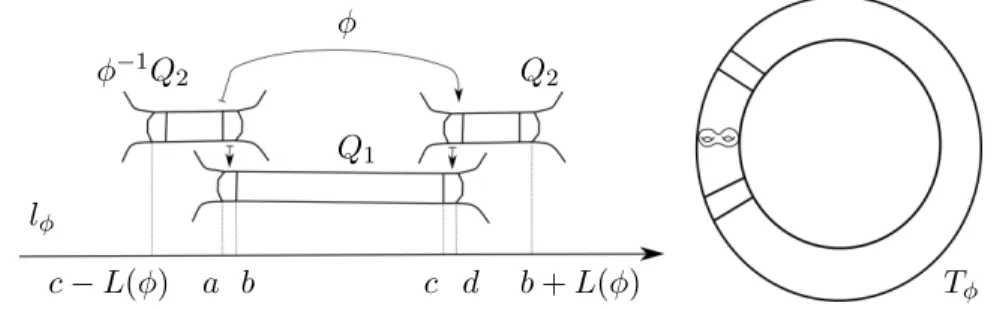
As an application of the same techniques, along the way, we give another proof of the following well-known result [19], [9] relating iterations of pseudo-Anosovs, volumes of quasi-fuchsian manifolds and mapping tori
Proposition 6. Let φbe a pseudo-Anosov mapping class. For every o∈ T the following holds:
lim
n→∞
vol (CC(Q(o, φno)))
n = vol (Tφ).
Small eigenvalues of random 3-manifolds. So far, we did not need to know much about how the -model metric (Mf, ρ) relates to the
underly-ing hyperbolic structure (Mf, σ). A careful inspection shows that we only
needed the fact that it almost computes its volume. The reason is that it is easy to manipulate the volume with the tools provided by Besson, Courtois and Gallot [4]. It is not straigthforward, instead, to use the same method to manipulate other invariants. This is the source of some of the difficulties we have to face next.
We now consider the spectral gap of the hyperbolic metric. This is a geometric invariant which is more sensitive of the metric than the volume. We recall that the spectral gap of (M, σ) is the smallest positive eigenvalue λ1(M, σ)>0 of the Beltrami-Laplace operator ∆σ on functions.
Theorem 7. We have the following
• Spectral gap: There exists a constant c=c(g)>0 such that
Pn[λ1(Mf)≤c/vol(Mf)2]n−→→∞1.
• Injectivity radius: For every >0 we have
Pn[inj(Mf)≤]n−→→∞1.
Theorem 7 is joint work with Ursula Hamenst¨adt and can be seen as a direct analogue for Heegaard splittings of a result of Baik, Gekhtman and Hamenst¨adt [1] for random mapping tori. In fact, we use Theorem 2 to import the strategy of [1] to the Heegaard splitting setting. We remark that the theorem holds also for the -model metric. In that case the proof can be copied almost word by word from [1].
This brings us to the main difficulty that we have to deal with which is exactly the comparison between the -model metric and the underlying hyperbolic structure. We develop a comparison technique which is tailored to the random 3-manifold setting. It is based on the method of natural maps introduced by Besson, Courtois and Gallot [4].
Before illustrating our technique, we pause for a second for a couple of comments on the qualitative and quantitative aspects of Theorem 7. The first one is that Theorem 7 identifies the coarse decay rate for the spectral
gap: Schoen [29] proved that there exists a universal constant a > 0 such that for all closed hyperbolic 3-manifoldsM we have
λ1(M)≥a/vol(M)2.
In the opposite direction, it is not possible to expect any inequality of the same form, that is independent of the genusgof a Heegaard splitting ofM. There are examples of sequences of manifolds (Mn)n∈N with the property that λ1(Mn) ≥δ for all n ∈N for some δ > 0 while vol(Mn) ↑ ∞ (see for
example [13]).
The second remark is that the decay rate in Theorem 7 is the fastest among all 3-manifolds with a Heegaard splitting of genus at most g as we now explain. Keeping in consideration the Hegaard genus, it is possible to give upper bounds on λ1(M): Combining work of Buser [14] and Lackenby [20], there exists a constant b(g) > 0 such that all closed hyperbolic 3-manifoldsM with Heegaard genus g also satisfy
λ1(M)≤b(g)/vol(M).
Moreover, the discrepancy between Schoen and the previous inequality is inevitable: There are sequences of hyperbolic 3-manifolds (Mn)n∈N with a splitting of genus at mostg and volume vol(Mn)↑ ∞that roughly saturate
both sides of the inequalities. In particular, for every > 0 there exists g, C and sequences (Mn) for which the Heegaard genus is bounded bygand
λ1(Mn)≥C/vol(Mn)1+ (see for example [1]).
The last remark is that a result of White [36] says that, in the presence of a uniform lower bound on the injectivity radius inj(M) ≥ > 0, the range for the spectral gap behaviour is coarsely the one allowed by Schoen inequality: There existsb(g, )>0 such thatλ1(M)≤b(g, )/vol(M)2. The second part of Theorem 7 shows that we cannot hope to apply White’s result in our setting: A random 3-manifold develops many thin parts.
We now briefly describe the main tool that we develop to compare the -model metric (Mf, ρ) to the hyperbolic structure (Mf, σ). Our technique
relies on a local analysis of Besson, Courtois and Gallot natural maps. Given two negatively curved metrics ρ and σ on M, one can produce a one-parameter family of natural maps {Fc : (M, ρ) → (M, σ)}c∈(a,b) which are homotopic to the identity and enjoy the following geometric properties
(i) They do not increase the volume, meaning that Jac(Fc)≤c.
(ii) At points where they are almost volume preserving, that is where Jac(Fc) is large enough, they are also almost isometric, that is dFc
is close to an isometry.
(iii) On uniform neighbourhoods of those points the map is also uniformly Lipschitz.
The range (a, b) in which we can choosec is determined by the curvature of ρ and σ. For an -model metric and a hyperbolic metric, c can be chosen
very close to 1. In particular
vol(Mf, ρ)/vol(Mf, σ) = 1 +o().
This implies that, in our case, the natural maps are forced to be almost volume preserving, and hence almost isometric, on large portions onM.
Combining with the explicit description of the-model metric (Mf, ρ) we
are able to deduce some useful information on the geometry of the hyperbolic structure (Mf, σ).
The idea is the following: Fix a compact 3-manifold with boundary U endowed with some fixed metric. We call such an object a geometric block. The prototypical example for us will be and a fundamental portion of a hyperbolic mapping torusTf, that isU =Tf−Σ where Σ⊂Tf is a standard
fiber with controlled geometry. Fix also a small number α∈(0,1).
Suppose that we can find pairwise disjoint isometric copiesU1,· · · , Uk of
U isometrically embedded in the -model metric (Mf, ρ) so that they eat a
definite proportion of the volume vol G j≤k Uj ≥αvol(Mf, ρ).
Since we also have vol(Mf, ρ)/vol(Mf, σ) = 1 +o(), if >0 is small enough
compared to α, then any natural map Fc : (Mf, ρ) → (Mf, σ) with c ' 1
must be almost volume preserving and, hence, locally almost isometric at some points in at least half of the componentsUj. For each of these
compo-nents, such local control can be upgraded to an almost isometric embedding ofUj by standard arguments of [4]. So we find many copies ofU uniformly
embedded also in (Mf, σ).
Ergodicity of a random walk [1] and the model manifold technology [25], [10] are the two main tools for finding such collections of blocks in the -model metric and hence ensure the presence of such blocks also in the hyperbolic metric. Having enough geometric blocks allows us to use the same arguments of [1] and get the upper bound for the spectral gapλ1(Mf, σ).
A particularly careful choice of blocks also gives us the following two con-sequences: As the middle pieceQhas many short curves, we immediately see that the injectivity radius inj(Mfn) drops to 0 almost surely. This provides a proof for the second assertion in Theorem 7.
In the opposite direction, we also see larger and larger geometric blocks where the injectivity radius is uniformly bounded from below. Hence, we can also choose basepoints xn ∈ Mfn such that the sequence (Mfn, xn) converges geometrically to a doubly degenerate structureQ∞on Σ×Rwith inj(Q∞)>0, i.e. Q∞ hasbounded geometry.
Commensurability and arithmeticity. The fact that the injectivity ra-dius can be made arbitrarily small and still we can choose basepoints so
that the sequence of random 3-manifolds converges to a doubly degenerate structure with bounded geometry has the following consequence:
Proposition 8. ForP-almost every (fn)n∈N the following holds
(1) There are at most finitely many 3-manifolds in the family(Mfn)n∈N that are arithmetic.
(2) There are at most finitely many 3-manifolds in the family(Mfn)n∈N that are in the same commensurability class.
The arguments for the proof of Proposition 8 are mostly borrowed from Biringer and Souto [5].
We observe that Dunfield and Thurston, using a simple homology com-putation have shown in [15] that their notion of random 3-manifold is not biased towards a certain fixed set of 3-manifolds. This means that for every fixed 3-manifoldM, only finitely many elements in the family (Mfn)n∈Ncan be diffeomorphic to M. Proposition 8 can be seen as a strengthening of their conclusions. It shows that the notion of random 3-manifolds is also not biased towards the class of arithmetic hyperbolic 3-manifolds and to the class of 3-manifolds which are commensurable to a fixed 3-manifoldM.
Constuction of model metrics. Having discussed some consequences of Theorem 2, we now illustrate what goes into its proof.
The construction is somehow implicit in the description of a -model metric (Mf, ρ). Recall that such a Riemannian manifold decomposes as
Mf = H1∪Ω1 ∪Q∪Ω2 ∪H2 and that its restriction to H1, Q and H2 is purely hyperbolic. We think of Ω1,Ω2 as the collar structure of the three larger piecesN1=H1∪Ω1,N2 = Ω2∪H2andQ= Ω1∪Q∪Ω2. Topologically, they are two handlebodies and one I-bundle.
The idea is to find, on each of the three topological piecesN1,N2andQ, a Riemannian metric which is purely hyperbolic in the interior and such that the geometry of large collars of ∂N1 and ∂N2 almost isometrically match the geometry of the collar of the corresponding boundary component of ∂Q. Moreover, we want to keep the size of the collars and the volumes under control. If we can do so, then we can patch together the Riemannian metrics and obtain a -model metric on Mf.
Such constructions are available in the literature (see [26], [27], [12], [11]), however we have to deal with one major difficulty, namely the fact that there is no a prioricontrol on the thick-thin decomposition of Mf. This piece of
information is implicitly assumed in the works mentioned above.
We will describe a route to overcome this issue that follows closely [12]. The geometric building blocksN1,N2andQfor the-model metric onMf
are portions of the convex cores of convex cocompact complete hyperbolic structures onHg and Σg×[1,2] respectively.
Notice that the gluing construction only requires a uniform control on the geometry near the boundaries of the blocks. The model manifold technology
developed by Minsky [25] and Brock, Canary and Minsky [10] provides such a control forQ. The same is not available in full generalities forN1,N2 and this is the main challenge in pursuing the gluing strategy that we described. We supply a uniform model for the collar geometry of ∂N1 and ∂N2 by slightly generalizing works of Brock, Minsky, Namazi and Souto [26], [12]. This is our main contribution here. In particular, we find conditions so that we can make sure that those collars are geometrically very close to a quasi-fuchsian hyperbolic structure on Σ×[1,2].
To this extent, we introduce a condition of relative R-relative bounded combinatoricsand large height for geometrically finite structures on handle-bodies. It differs from the R-bounded combinatorics condition of [26] and [12] only because it is a local condition.
Theorem 9. For every R >0 and > 0 there exists h=h(R, ) >0 such that if Mf has relative R-bounded combinatorics and height at least h then
the Heegaard splitting Mf admits a-model metric.
Compared to [26], [12], the main novelty is that we allow a non trivial thick-thin decomposition and require only a local control.
Ergodicity of the random walk implies that the condition of having R-relative bounded combinatorics is generic, so the previous discussion is ap-plicable to random 3-manifolds.
We also remark that, in the random setting, it follows from the construc-tion that the middle pieceQclosely resembles a large portion of the convex core of the quasi-fuchsian manifold Q(o, f o) where o ∈ T is a base point carefully fixed once and for all.
Hyperbolization and uniform models. Up to now, the existence of a hyperbolic structure was guaranteed by Maher’s theorem which rests upon the solution of the geometrization conjecture by Perelman.
We now describe aconstructiveproof of Maher’s result that bypasses the use of Ricci flow with surgery.
Given the amount of information that can be extracted from the model manifold technology, it is desirable, for random 3-manifolds, to have not only a hyperbolic metric, but also a uniform bilipschitz model for it with the structure of a -model metric. This is indeed the case: We have the followingeffective version of Theorem 1
Theorem 10. For every 0< <1/2 and K >1 we have
Pn[Mf has a hyperbolic metric K-bilipschitz to a-model metric]n−→→∞1.
Our methods follow closely [12] and [11] where uniform -model metrics are constructed for special classes of 3-manifolds.
The idea is the following: We can obtain a hyperbolic metric onMf by a
hyperbolic cone manifold deformation from a finite volumedrilledmanifold
of Σ⊂Mf. We consider 3-manifolds
M=Mf −(P1× {1} ∪P2× {2} ∪P3× {3} ∪P4× {4})
where Pj is a pants decomposition of the surface Σ× {j}. A finite volume
hyperbolic metric on such a manifold can be constructed explicitly by gluing together the convex cores of twomaximally cuspedhandlebodiesH1, H2 and three maximally cuspedI-bundles Ω1, Q,Ω2.
M=H1∪Ω1∪Q∪Ω2∪H2.
Most of our work consists of finding suitable pants decompositions for which the Dehn surgery slopes needed to pass from M toMf satisfy the
assump-tions of the effective Hyperbolic Dehn Surgery Theorem [18]. In order to find them we crucially need two major tools: The work of [16] on the geom-etry of hyperbolic handlebodies and ergodic properties of the random walks proved by Baik, Gekhtman and Hamenst¨adt [1].
In order to provide a uniform bilipschitz control we exploit, instead, er-godic properties of the random walk and drilling and filling theorems by Hodgson and Kerckhoff [18] and Brock and Bromberg [8].
In the next paragraphs we present two further geometric applications that use the control given by Theorem 10.
Diameter growth. As a first application we compute the coarse growth rate of the diameter of random 3-manifolds.
Proposition 11. There exists c >0 such that
Pn[diam(Mf)∈[n/c, cn]]n−→→∞1.
The coarsely linear upper bound follows from a theorem by White [35] relating the diameter to the presentation length of π1(Mf). It is not
dif-ficult to see that the latter grows at most linearly in a family of random 3-manifolds. The lower bound comes from the-model metric structure.
Geometric limits. We have already established that it is possible to obtain a doubly degenerate structure on Σ×Rwith bounded geometry as a limit, in the pointed geometric topology (see Chapter E.1 of [2]), of a sequence of random 3-manifolds.
Using Theorem 10, it is possible to show that, in fact, it is possible to deform a sequence of random 3-manifolds towards any pointed doubly de-generate structure on Σ×R. This is the content of the next proposition
Proposition 12. For every φ pseudo-Anosov with associated hyperbolic mapping torus Tφ and for P-almost every (fn)n∈N there exists a sequence of base pointsxn∈Mfn such that the sequence(Mfn, xn) converges geomet-rically to the infinite cyclic covering of Tφ.
The family of infinite cyclic coverings of hyperbolic mapping tori is dense in the space of doubly degenerate structures endowed with the pointed geo-metric topology. This follows from two facts: The first one is that the subset ofPML × PML consisting of the pairs (λ−(φ), λ+(φ)) of repelling and at-tracting fixed points of pseudo-Anosov elements φ is dense. The second one is Thurston’s Double Limit Theorem [30] combined with the Ending Lamination Theorem [25], [10].
A larger class of random walks. We conclude by just adding a couple of words on the assumptions on the probability measure µ that drives the random walk.
We recall that we only considered probability measures whose finite sup-port generates the entire mapping class group. These assumptions can be considerably weakened and still obtain model metrics and convergence re-sults as in Theorems 2, 4 and 5 but we have to distinguish between mapping tori and Heegaard splittings.
In the mapping torus case (and also in Theorem 5), it is enough that the subgroup generated by the support of µ contains two pseudo-Anosov elements that act as independent loxodromics on the curve graph. In the Heegaard splitting case, we further require that the two pseudo-Anosov el-ements act as independent loxodromics also on the handlebody graph. We refer to Maher and Tiozzo [24] and Maher and Schleimer [23] for more de-tails on random walks on these spaces. In such higher generalities the proofs will be word by word the same, no change is needed.
Outline. This thesis is divided into three parts.
The first part contains the articleSmall eigenvalues of random 3-manifolds
[16] in which the existence of an -model metric is established as in Theo-rem 2 and TheoTheo-rem 9 and then used to control the first positive eigenvalue of the Laplacian as stated in Theorem 7. This is joint work with Ursula Hamenst¨adt.
The second part corresponds to the articleVolumes of random 3-manifolds
[33] where we prove a law of large numbers for the volumes of a family of random 3-manifolds. The results discussed in this part are Theorem 4, Theorem 5 and Proposition 6.
The last chapter is the article Uniform models for random 3-manifolds
[34]. There, we produce hyperbolic metrics uniformly bilipschitz to-model metrics on random Heegaard splittings (as in Theorems 1 and 10). As an application, we coarsely identify, in Proposition 11, the coarse growth rate of the diameter of random 3-manifolds. We also prove Proposition 8 about arithmeticity and commensurability classes of random 3-manifold.
The three different parts are presented in their preprint form. As such, they are as self-contained and as independent of each other as possible. Their conclusions and ideas are discussed organically in the introduction.
Acknowledgements. I want to thank Ursula Hamenst¨adt for her guidance and patience. This work is very much indebted to her insight and ideas and it would certainly have never been completed without many long discussions. I want to thank Sebastian Hensel for his interest in this work, for the possibility to talk about it and for accepting to be in my defense committee. I want to thank Giulio Tiozzo for discussing the problem of the linearity of the volume for random 3-manifolds with me.
I acknowledge the financial support of the ERC grant Moduli and of the Max Planck Institut f¨ur Mathematik of Bonn.
I also take the chance to thank Andrea Bianchi, Bram Petri, Beatrice Pozzetti, Federica Fanoni, Luca Battistella for their friendship and help, for infinitely many conversations, mathematical and non-mathematical, and, in general, for being part of three enjoyable years.
Finally, I want express my infinite gratitude to my mother, father and my brother for their steady unconditional support.
References
[1] H. Baik, I. Gekhtman, U. Hamenst¨adt, The smallest positive eigenvalue of fibered hyperbolic 3-manifolds, Proc. Lond. Math. Soc.120(2020), 704-741.
[2] R. Benedetti, C. Petronio, Lectures on hyperbolic geometry, Universitext, Springer Verlag, Berlin 1992.
[3] L. Bers,Simultaneous uniformization, Bul. Amer. Math. Soc.66(1960), 94-97. [4] G. Besson, G. Courtois, S. Gallot, Lemme de Schwarz r´eel et applications
g´eom´etriques, Acta Math.183(1999), 145–169.
[5] I. Biringer, J. Souto,A finiteness theorem for hyperbolic 3-manifolds, J. Lond. Math. Soc.84(2011),
227-242-[6] J. Brock,Weil-Petersson distance and volumes of mapping tori, Comm. Anal. Geom.
11(2003), 987-999.
[7] J. Brock,The Weil-Petersson metric and volumes of 3-dimensional hyperbolic convex cores, J. Amer. Math. Soc.16(2003), 495-535.
[8] J. Brock, K. Bromberg,On the density of geometrically finite Kleinian groups, Acta Math.192(2004), 33-93.
[9] J. Brock, K. Bromberg,Inflexibility, Weil-Petersson distance, and volumes of fibered 3-manifolds, Math. Res. Lett.23(2016), 649-674.
[10] J. Brock, R. Canary, Y. Minsky,The classification of Kleinian surface groups, II: The Ending Lamination Conjecture, Ann. Math.176(2012), 1-149.
[11] J. Brock, N. Dunfield, Injectivity radii of hyperbolic integer homology 3-spheres, Geom. Topol.19(2015), 497-523.
[12] J. Brock, Y. Minsky, H. Namazi, J. Souto,Bounded combinatorics and uniform models for hyperbolic 3-manifolds, J. Topology9(2016), 451-501.
[13] M. Burger, P. Sarnak,Ramanujan duals II, Invent. Math.106(1991), 1-11.
[14] P. Buser,A note on the isoperimetric constant, Ann. Sci. Ec. Norm. Sup.15(1982), 213-230.
[15] N. Dunfield, W. Thurston, Finite covers of random 3-manifolds, Invent. Math.
166(2006), 457-521.
[16] U. Hamenst¨adt, G. Viaggi, Small eigenvalues of random 3-manifolds, arXiv:1903.08031.
[17] J. Hempel, 3-manifolds as viewed from the curve complex. J. Topology 40(2001), 631-657.
[18] C. Hodgson, S. Kerckhoff,Universal bounds for hyperbolic Dehn surgery, Ann. Math.
162(2002), 367-421.
[19] S. Kojima, G. McShane,Normalized entropy versus volume for pseudo-Anosov, Geom. Topol.22(2018), 2403-2426.
[20] M. Lackenby, Heegaard splittings, the virtual Haken conjecture and Property (τ), Invent. Math.164(2006), 317-369.
[21] J. Maher, Random walks on the mapping class group, Duke Math. J. 156(2011), 429-468.
[22] J. Maher,Random Heegaard splittings, J. Topology3(2010), 997-1025.
[23] J. Maher, S. Schleimer, The compression body graph has infinite diameter, arXiv:1803.06065.
[24] J. Maher, G. Tiozzo, Random walks on weakly hyperbolic groups, J. Reine Angew. Math.742(2018), 187-239.
[25] Y. Minsky,The classification of Kleinian surface groups, I: Models and bounds, Ann. Math.171(2010), 1-107.
[26] H. Namazi, Heegaard splittings and hyperbolic geometry, PhD Thesis, Stony Brook University, 2005.
[27] H. Namazi, J. Souto, Heegaard splittings and pseudo-Anosov maps, Geom. Funct. Anal.19(2009), 1195-1228.
[28] I. Rivin, Statistics of random 3-manifolds occasionally fibering over the circle, arXiv:1401.5736v4.
[29] R. Schoen,A lower bound for the first eigenvalue of a negatively curved manifold, J. Diff. Geom.17(1982), 233-238.
[30] W. Thurston, Hyperbolic structures on manifolds, II: Surface groups and 3-manifolds which fiber over the circle, arXiv:math/9801045.
[31] W. Thurston,Three dimensional manifolds, Kleinian groups and hyperbolic geometry, Bull. Amer. Math. Soc.6(1982), 357-381.
[32] G. Tian,A pinching theorem on manifolds with negative curvature, unpublished. [33] G. Viaggi,Volumes of random 3-manifolds, arXiv:1905.04935.
[34] G. Viaggi,Uniform models for random 3-manifolds, arXiv:1910.09486. [35] M. White,A diameter bound for closed hyperbolic 3-manifolds, arXiv:0104192. [36] N. White, Spectral bounds on closed hyperbolic 3-manifolds, J. London Math. Soc.
SMALL EIGENVALUES OF RANDOM 3-MANIFOLDS
URSULA HAMENST ¨ADT AND GABRIELE VIAGGI
Abstract. We show that for every g ≥2 there exists a number c =
c(g)>0 such that the smallest positive eigenvalue of a random closed 3-manifoldM of Heegaard genusgis at mostc(g)/vol(M)2.
1. Introduction
By celebrated work of Perelman, any closed oriented aspherical atoroidal 3-manifold admits a hyperbolic metric, and such a metric is unique by Mostow rigidity1. In recent years, there was considerable progress in the understanding of the relation between geometric and topological invariants of such a manifold. The program to construct an explicit combinatorial model which describes the geometry up to uniform quasi-isometry turned out to be particularly fruitful [40, 10, 11], but it is far from completed.
The main purpose of this article is obtain an understanding of geometric and topological invariants forrandom hyperbolic 3-manifolds in the sense of Dunfield and Thurston [16]. Namely, fix a genusg≥2. A closed 3-manifold of Heegaard genus at most g can be obtained by gluing two handlebodies of genus g along the boundary with a diffeomorphism φ. The resulting 3-manifold M only depends on the isotopy class of φ, and it is aspherical atoroidal and hence hyperbolic if φis sufficiently complicated. Thus hyper-bolic 3-manifolds of Heegaard genusgcorrespond to suitable elements of the mapping class group Mod(Σ) of the boundary surface Σ of a handlebody of genusg (in fact, they correspond to double cosets in this group, see [16]).
Now let us choose a symmetric probability measure on Mod(Σ) whose finite support generates Mod(Σ). This measure generates a random walk on Mod(Σ), and hence it induces a notion of a random 3-manifold, glued from two handlebodies with a random gluing map. A random 3-manifold is hyperbolic [16] and hence we can study the behavior of geometric invariants of such random hyperbolic 3-manifoldsM.
Our main technical result (Theorem 6.7) constructs for a 3-manifold ob-tained from a gluing map with some additional properties a Riemannian metric of sectional curvature close to −1 everywhere and different from
Date: April 2, 2019.
AMS subject classification: 58C40, 30F60, 20P05
Both authors were partially supported by ERC grant ”Moduli”. 1For the bibliography of this part of the thesis see page 70.
−1 only in geometrically controlled regions where the injectivity radius is bounded from below by a universal constant. These constraints are fulfilled for random gluing maps.
We use this construction to obtain information on the spectrum of the Laplacian of a random hyperbolic 3-manifold M. List the eigenvalues as 0 = λ0(M) < λ1(M) ≤ λ2(M) ≤ λ3(M) ≤ . . ., with each eigenvalue re-peated according to its multiplicity. By [44] and [21], there exists a universal constantχ >0 such that
λ1(M)≥ χ
vol(M)2 and λvol(M)/χ(M)≥χ
for every closed hyperbolic 3-manifold M. Manifolds which fibre over the circle provide examples for which these estimates are essentially sharp. We refer to the introduction of [1] for a more comprehensive discussion.
On the other hand, it follows from the work of Buser [12] and Lackenby [26] that there exists a numberb(g)>0 such that for a hyperbolic 3-manifold M of Heegaard genusg, there is a bound
λ1(M)≤ b(g)
vol(M).
Hyperbolic 3-manifolds constructed from expander graphs have arbitrarily large volume, yet their smallest positive eigenvalue is bounded from below by a universal constant. Hence in this estimate, the dependence of the constant b(g) on the Heegaard genusg can not be avoided.
Under geometric constraints, one obtains better estimates. White [49] showed that there is a numbera(g)>0 such thatλ1(M)≤a(g)/vol(M)2 if M is of Heegaard genus g and the injectivity radius of M is bounded from below by universal constant. The same holds true for random hyperbolic 3-manifolds which fibre over the circle, with fibre genusg [1].
Using the model metric for random hyperbolic 3-manifolds as our main tool we show.
Theorem 1. For every g≥2 there exists a number c(g)>1 such that λ1(M)≤
c(g)
vol(M)2 andλvol(M)/c(g)(M)≤c(g) for a random hyperbolic 3-manifold of Heegaard genus g.
Here the upper bound forλvol(M)/c(g)(M) is a straightforward consequence of domain monotonicity with Dirichlet boundary conditions. For the upper bound for λ1(M), we expect that the dependence of the constantc(g) on g can not be avoided.
Strategy of the proof. As mentioned above, our main technical result is Theorem 6.7 which provides of an explicit Riemannian metric of curvature close to −1 on a 3-manifold of Heegaard genusg with some constraints on the gluing map. Constructions of geometrically controlled model metrics
appear frequently in the literature, for example as a main tool in [42] and in [41]. For doubly degenerate hyperbolic 3-manifolds whose fundamental group is isomorphic to the fundamental group of a closed surface, there is a completely explicit combinatorial model for the geometry [40, 10]. More recently these results were used to describe explicitly the geometry of hy-perbolic 3-manifolds with a lower bound on the injectivity radius and some topological constraints [11].
We can not apply the constructions in [11] as there are no lower bounds for the injectivity radius of a random hyperbolic 3-manifoldM. Instead we use properties of the random walk to locate regions in a random 3-manifold which are diffeomorphic to a trivial I-bundle over a closed surface and such that a combinatorial model would predict a uniform lower bound on the injectivity radius in those regions. This is the constraint on the gluing map required in Theorem 6.7. The model metric is then constructed by cutting M open at two such regions and by using information on suitable model metrics for the pieces.
For random hyperbolic 3-manifolds M, we find that the spectrum of the model metric fulfills the properties stated in Theorem 1.
The last step consists in comparing the model metric onM and the hyper-bolic metric. A result of Tian [47] implies that the model metric isC2-close to the hyperbolic metric. As this work is neither published nor available in electronic form, we prove a weak substitute which is sufficient for the proof of Theorem 1. Our argument is based on the methods introduced in [4].
Organization of the article. In Section 2 we collect some properties of the pointed geometric topology for 3-dimensional Riemannian manifolds which are used later on.
In Section 3 we introduce a relative version of bounded combinatorics and set up sufficient conditions for the construction of a model metric. This construction depends on the existence oflarge thick collars, a property which is introduced in Section 4.
Sections 5 and 6 are devoted to the proof of Theorem 6.7 which provides a model metric for a hyperbolic 3-manifold of fixed Heegaard genus with some additional properties. In Section 7 we show that random hyperbolic 3-manifolds have the properties required in Section 6, and in Section 8 we relate the model metric to the hyperbolic metric using tools from [4]. The information on the hyperbolic metric we obtain then leads to Theorem 1.
2. Hyperbolic structures on handlebodies
The goal of this section is to collect some results from the deformation theory of convex cocompact hyperbolic metrics on handlebodies in the form used later on. We also introduce some notations which are used throughout the article.
We begin with making precise what we understand by looking at a convex cocompact hyperbolic handlebody from the point of view of the boundary of the convex core. We give a quantitative description of the notion of a large collar with bounded geometry (alarge-thick collar). As a preparation for Section 4, we describe some basic general compactness properties of the geometric topology.
Fix, once and for all, a genus g ≥ 2. Let H be a handlebody of genus g, with boundary surface Σ := ∂H. We fix on H an orientation, and we coherently orient Σ as the boundary ofH.
A marked hyperbolic structure on the handlebody H is a quotient N =
H3/Γ of hyperbolic 3-space by a discrete free subgroup Γ < PSL
2(C) = Isom+ H3, together with a homeomorphism (the marking) φ: int (H)−→
N. We say that the marked structuresφ: int (H)−→N andψ: int (H)−→ N0 areequivalent if there exists an isometryf :N −→N0 such thatf◦φis isotopic toψ.
2.1. Parametrization of marked convex cocompact structures. We denote by T = T(Σ) the Teichm¨uller space of marked hyperbolic metrics on Σ, and byM=M(Σ) = Mod(Σ)\T(Σ) the moduli space of hyperbolic metrics on Σ.
By classical results due to Bers, Kra, Maskit, Sullivan and others, so-called convex cocompact hyperbolic structures on the handlebody H are parametrized by a parameter that lies in the Teichm¨uller space T of the boundary surface.
Namely, let N = H3/Γ be a hyperbolic structure on H. Associated to Γ we have the limit set Λ ⊂ ∂H3 which consists of the points at infinity of a Γ−orbit closure, and the domain of discontinuity ΩΓ = ∂H3−Λ, the complement of the limit set. The group Γ, isomorphic to a free groupFg of rank g, acts freely and properly discontinuously both on the convex hull of the limit setCH(Λ)⊂H3 and on the domain of discontinuity ΩΓ⊂∂H3. In the remainder of this section we will always assume that ΩΓ6=∅.
The quotient
CC(N) :=CH(Λ)/Γ
is the convex core of N. It is a convex topological submanifold of N, pos-sibly with boundary. The manifold N is called convex cocompact ifCC(N) is compact. The complement N − CC(N) is naturally homeomorphic to ∂CC(N)×(0,∞).
The quotient ∂cN := ΩΓ/Γ is the (unmarked)conformal boundary of N (we can think of it as a point in moduli space). AsN is convex cocompact, ∂cN is homeomorphic to the closed surface Σ =∂H. The conformal
bound-ary is equipped with a natural conformal structure and hence a hyperbolic metric (which we refer to as the Poincar´e metric) coming from the fact that
Γ acts via M¨obius transformations on ∂H3. The quotient N =H3∪ΩΓ/Γ =N ∪∂cN
gives a natural compactification ofN.
Using a marking φ: int (H) −→ N, the isotopy class of the inclusion of the boundary Σ :=∂H,→ H determines an isotopy class of an embedding Σ ,→ N. We use this isotopy class to give a marking to the conformal boundary ∂cN and to the boundary of the convex core ∂CC(N).
In this terminology, Bers parametrization can be stated as follows: Equiv-alence classes of marked convex cocompact structures are parametrized by the marked conformal boundary. Given a marked conformal boundary X ∈ T, we denote by H(X) the corresponding marked convex cocompact hyperbolic handlebody.
2.2. The boundary of the convex core. As before, let N =H/Γ be a convex cocompact hyperbolic structure onH. Then the boundary∂CC(N)⊂
N of the convex core is an embedded pleated surface.
Definition (Pleated Surface, Thurston [46]). LetM be a hyperbolic 3-ma-nifold and let us fix a homotopy class of mapsj: Σ→M. A pleated surface in the homotopy class of j consists of the following data:
• A hyperbolic metric σ on Σ.
• A path-isometry f : (Σ, σ) → M homotopic to j such that every point x ∈Σ is contained in a geodesic segment which is mapped to a geodesic inM.
Associated to every pleated map f : (Σ, σ) → M there is a geodesic lamination λ ⊂ Σ, called the pleating locus with the following property. Every leaf of λ is mapped to a geodesic by f, and the restriction of f to every component of Σ−λ, is a locally isometric immersion. We say that f realizesλ⊂Σ inM within the homotopy classj. For more on laminations and pleated surfaces we refer the reader to Chapter I.5 of [15].
There is a naturalnearest point retraction(see Chapter II.1.3 of [15]) from the conformal boundary to the boundary of the convex core r : ∂cN −→
∂CC(N). With respect to the induced markings on the conformal boundary and on the boundary of the convex core,r lies in the homotopy class of the identity.
The following result of Bridgeman and Canary provides control of the boundary of the convex core when we have a good understanding of the geometry of the conformal boundary:
Theorem 2.1 (Bridgeman-Canary, [8]). There are maps J, G : (0,∞) → (1,∞) such that the following holds: Let Γ <PSL2(C) be a finitely gener-ated, non-elementary, torsion free Kleinian group. Suppose that the length, measured with respect to the Poincar´e metric, of every curve in the confor-mal boundary ΩΓ/Γ which is compressible in the 3-manifold H3∪ΩΓ
is bounded from below by ρ >0. Then the nearest point retraction from the conformal boundary to the boundary of the convex core is J(ρ)−Lipschitz and admits a G(ρ)−Lipschitz homotopy inverse.
2.3. Limits of hyperbolic manifolds. Let us choose for every (marked) convex cocompact structure on the handlebodyH a basepointx∈∂CC(N) on the boundary of the convex core. We then can talk about a marked pointed convex cocompact handlebody.
Definition (Geometric Convergence). A sequence{(Mn, mn)}n∈Nof poin-ted hyperbolic 3-manifolds is said toconverge in the pointed geometric topol-ogy to a pointed hyperbolic 3-manifold (M∞, m∞) if the following condi-tions are satisfied. For every R > 0, ξ > 0 there are numbers n(R, ξ) >0, and for every n ≥ n(R, ξ) there exists a map (the approximating map) k:Un⊂M∞→Mn such that
• k is defined on the ball BM∞(m∞, R) of radius R centered at the
basepoint m∞ ofM∞ and sends this basepoint to the base point of Mn.
• the restriction of k to the ball BM∞(m∞,R2) isξ-close to an isome-try in the C2-topology: The metric tensor ρ
∞ of M∞ and the
pull-back k∗ρn by k of the metric tensor ρn of Mn are ξ-close in the
C2-norm on 2−tensors on the ball B
M∞ m∞,R2 which we denote by ||k∗ρn−ρ∞||C2,B m∞,R 2 .
To be more precise, let∇∞ be the Levi-Civita connection forρ∞. Define
||k∗ρn−ρ∞||C2,B m ∞,R2 =||k∗ρn−ρ∞|| C0,B m ∞,R2 +||∇∞(k∗ρn)||C0,B m ∞,R2 +||∇∞∇∞(k∗ρn)|| C0,B m ∞,R2 .
We then say that the restriction ofk toB(m∞, R/2) is ξ-almost isometric. Note that this definition of geometric convergences is slightly more re-strictive than what is found in the literature (see e.g. Chapter E of [2]). We shall make use of the following compactness result for geometric convergence (Theorem E.1.10 of [2]).
Theorem2.2. Suppose that{(Mn, mn)}n∈N is a sequence of pointed
hyper-bolic 3-manifolds such that there is a uniform positive lower boundη >0 on the injectivity radius at the base points mn. Then there exists a subsequence
that converges in the geometric topology to a pointed hyperbolic 3-manifold (M∞, m∞).
We observe next that in combination withMargulis’ Lemma (see e.g. [2]), Theorem 2.1 implies that if the conformal boundary of a convex cocompact hyperbolic structureN on a handlebodyHis-thick in the Poincar´e metric (i.e. its injectivity radius is at least), then there is a uniform lower bound, only depending on > 0 and g = g(Σ), on the injectivity radius of N at points that are close to the boundary of the convex coreCC(N). This enables us to take geometric limits.
For the formulation of this fact, for sufficiently small >0 we denote by
T⊂ T the subset of Teichm¨uller space of all marked hyperbolic metrics on Σ
with injectivity radius at least, and we letM = Mod(Σ)\Tbe the-thick
part of moduli space. Furthermore, let injx(N) be the injectivity radius of a hyperbolic manifoldN at the pointx, and let inj(N) = infx{injx(N)|x∈
N}the global injectivity radius of N.
Lemma 2.3. For every > 0 and g ≥ 2 there exists η = η(, g) > 0 such that the following holds: Let N be a convex cocompact hyperbolic structure onH. If ∂cN ∈ M then infx∈∂CC(N){injx(N)} ≥η.
In the proof and in the sequel we use the following notations:
Notation. If X is a hyperbolic surface and γ :S1 → X is a smooth closed curve, then we denote byL(γ) the length of γ, and byLX(γ) the length of the geodesic representative of
γ onX. For a curve γ in a hyperbolic 3-manifoldM we use the notationl(γ) and lM(γ) for the analogous quantities.
Proof. By Theorem 2.1, we have that every simple closed curve on the boundary of the convex core γ ⊂ ∂CC(N) has length (with respect to the induced hyperbolic metric)
L∂CC(N)(γ)≥ 1
G()L∂cN(γ)≥ 2 G() as inj(∂cN)≥.
Hyperbolic trigonometry shows that there exists a uniform upper bound for the diameter of ∂CC(N) in the intrinsic metric, say diam∂CC(N) ≤D where D = D(, g) only depends on > 0 and g ≥ 2. Since the inclusion ∂CC(N) ⊂ N is 1−Lipschitz by definition of the intrinsic path-metric, we have the same control on the diameter when we compute distances in N.
Let3 >0 be a Margulis constant for hyperbolic manifolds in dimension 2 and 3. By Margulis’ Lemma, for some small number ρ < 3 the ρ−thin part N(0,ρ] := N − {x∈N |injxN > ρ} of N is a disjoint union of Mar-gulis tubes, i.e. metric tubular neighbourhoods of simple closed geodesics of length smaller than ρ.
Having bounded diameter and carrying all the information about the fundamental group of H, the surface ∂CC(N) cannot penetrate deeply into a Margulis tube. Namely, letγ ⊂N be the core geodesic of the ρ-Margulis tube containingx∈∂CC(N). Standard hyperbolic geometry yields that the distance between the boundary of the ρ−Margulis tube and the boundary of the3−Margulis tube ofγ grows to∞ asρapproaches 0. In particular, if ρ is sufficiently small then by the diameter bound for ∂CC(N), this surface is entirely contained in the3-Margulis tube. This contradicts the fact that the inclusion ∂CC(N) ,→ N is π1−surjective. Hence the injectivity radius of N at points in ∂CC(N) is bounded from below by a universal positive
By Lemma 2.3 and compactness of pleated surfaces (see section I.5.2 of [15], in particular Theorem I.5.2.2), given a sequence of triples
{(Nn, jn:Xn⊂ M →∂CC(Nn), xn)}n∈N
consisting of convex-cocompact hyperbolic structures, corresponding (plea-ted surface parametrizations of the) boundaries of the convex cores and basepoints such that the conformal boundary is-thick, we can always ex-tract a subsequence (say the whole sequence) that converges in the geometric topology to a triple (N∞, j∞:X∞→N∞, x∞), consisting of a hyperbolic 3-manifold, a pleated surface and a common basepoint, in the following sense:
• The sequence of pointed 3-manifolds (Nn, xn) converges to (N∞, x∞). • The sequence of pointed hyperbolic surfaces (∂CC(Nn), xn) converges
to the pointed hyperbolic surface (X∞, x∞). Observe that, by The-orem 2.1, ∂CC(Nn) has a uniform lower bound on the injectivity
radius and a uniform upper bound on the diameter. In particular, the surfaces Xn are contained in a compact subset of moduli space,
and the surface X∞ ∈ Mis an accumulation point of the sequence (Xn). In particular, it shares the same uniform bounds on the
injec-tivity radius and the diameter.
• The pleated surface embeddings ∂CC(Nn) ,→ Nn, which we denote
by jn, converge to a pleated surface j∞:X∞ →N∞. The diagram
where all the maps respect the basepoints, and the vertical arrows are the approximating maps provided by the geometric convergence,
∂CC(Nn) jn / /Nn X∞ j∞ / / φn O O N∞ kn O O
commutes up to local (pointed) homotopies, i.e. those homotopies that respect the base points and take place in small neighbourhoods of the images of the pleated surfaces.
• Lastly, we also recall that ∂CC(Nn) and X∞ come together with a
marking (as in the definition of pleated surface), i.e. they are isomet-rically identified with Σ, σ∂CC(Nn) and (Σ, σ∞). These markings consist of collections of curves whose lengths are uniformly bounded for the induced hyperbolic metrics. We can assume that the composi-tion of the identificacomposi-tion Σ, σ∂CC(Nn)'∂CC(Nn) with the inclusion
in Nn is isotopic to the marking of Nn, and that the marked (and
3. Relative bounded combinatorics
Bounded combinatorics is a combinatorial condition which translates into explicit geometric control of the hyperbolic metric on the convex cocompact handlebody near the boundary of its convex core.
Relative versions of bounded combinatorics were introduced in [41], [42] and [11]. We are interested in bounded combinatorics relative to a decorated handlebodyH, where the decoration is either a markingµon∂Hor a point X ∈ T, which we can think of as a “fixed convex cocompact structure” on
H. We recall that, if X ∈ T, then the geometric realization H(X) is the convex cocompact handlebody whose marked conformal boundary equals X.
Following ideas of Minsky [40] and of Brock-Canary-Minsky [10], our goal is to construct for a random 3-manifold M a model metric which is close to the hyperbolic metric and such that on a submanifold M0 of M whose volume is bigger than a definite proportion of the volume ofM, this metric can explicitly be described.
Our construction is a variation of earlier constructions of [41], [42] and [11]. Namely, we glue the model metric from hyperbolic metrics on pieces with large overlap on which the metrics have large injectivity radius and are very close. The condition we need to successfully glue these metrics on the overlap to a metric which is close to a hyperbolic metric can be described as “bounded combinatorics and large height”.
Our setup, however, is different from the setup in these earlier work as we can not assume any global control of the injectivity radius, i.e. unbounded geometry appears. The purpose of this section is to provide the control needed in the sequel.
We begin with collecting the essential facts about coarse geometry and Gromov hyperbolic spaces, in particular about the geometry of the curve graph and thedisk graph.
3.1. Coarse Geometry. A map f : (X, dX) → (Y, dY) between metric
spaces is an (L, C)−quasi-isometric embedding if for everyx, x0 ∈X 1
LdX(x, x
0)−C≤d
Y(f(x), f(x0))≤LdX(x, x0) +C.
A parametrized (L, C)−quasi-geodesic segment, ray or line is an (L, C)-quasi-isometric embedding of an interval, a half line or the entire real line
R. Later on we will have to deal also with unparametrized (L, C)− quasi-geodesic segments, rays and lines which are maps f : I ⊂ R −→ (X, dX)
such that there exists a homeomorphism φ from an interval I0 ⊂ R onto the intervalI with the property that the compositionf◦φ:I0 −→(X, dX)
is a (L, C)−quasi-isometric embedding (the intervals I, I0 can be finite or infinite).
3.2. Curve and Disk Graphs. Masur and Minsky proved in [32] that the curve graph C := C(Σ) of the closed surface Σ of genus g ≥ 2 is a Gro-mov hyperbolic space of infinite diameter, and Klarreich [24] identified the Gromov boundary ∂∞C =∂∞C(Σ) with the space EL=EL(Σ) of minimal filling unmeasured laminations (see also [19] for a different approach).
Definition (Gromov Product and Convergence). Given α, β, γ ∈ C, the quantity
(α|β)γ := 1
2[d(α, γ) +d(β, γ)−d(α, β)]
is the Gromov product ofα, βbased atγ. A sequence{αn}n∈N⊂ Cconverges at infinity to a point in∂∞C if and only if for some base pointγ (and hence for any) we have lim infn,m→∞(αn|αm)γ → ∞. If {αn}n∈N converges at infinity and {βn}n∈N satisfies lim infn,m→∞(αn|βm) = ∞, then {βn}n∈N converges to the same point in∂∞C.
For material on Gromov products and Gromov boundaries we refer the reader to Section 3 of Chapter III.H of [9].
The geometry of the curve graph is coarsely tied to the geometry of Te-ichm¨uller space. There is a (coarsely well-defined) Mod (Σ)-equivariant map
Υ :T → C,
called thesystole map, that associates to every marked hyperbolic structure X ∈ T a shortest geodesic on it Υ(X). It follows from Masur-Minsky [32] that there exist constants L≥1, C ≥0 only depending on Σ such that for every Teichm¨uller geodesic l:I → T (here I can be an interval, a half-line or the whole real line) the composition Υ◦l :I → C is an unparametrized (L, C)-quasi-geodesic. Moreover, if we restrict our attention to the -thick partT of Teichm¨uller space, then the situation improves: In [20] it is shown
that for every >0 there existL≥1, C ≥0 such that iflis parametrized
by arc length on an interval of lengthl(I) ≥L and ifl(I) ⊂ T then Υ◦l
is aparametrized (L, C)-quasi-geodesic.
Thedisk graph Dassociated to the identification Σ =∂His the subgraph of C spanned by disk-bounding curves. Masur and Minsky showed in [34] that the disk graphDis a quasi-convex subset of the curve graphC. Being quasi-convex, by hyperbolicity ofC, there is a coarsely defined nearest point projection πD :C −→ D.
3.3. Subsurface projection and Bounded Combinatorics. An essen-tial tool for describing the geometry of the curve graph is the notion of subsurface projection introduced by Masur-Minsky in [33]: For every proper essential subsurface W ⊂Σ (with some care for annuli and pairs of pants) and every point α ∈ C ∪ (∂∞C = EL), there is a subsurface projection πW(α)⊂ C(W) which consists of the (possibly empty) subset of C(W) of all
We can also define subsurface projections for markings (taking the projec-tion of the marking as a subset ofC). All the markingsµ on Σ we consider arecomplete, i.e. they are given, as a subset ofC, by apants decomposition, called thebase of the marking, and for every curveαin the base a transver-sal tα, that is, a simple closed curve which intersects α essentially in the
least possible number of points (either one or two points) and does not inter-sect the other curves in the base. The total geometric interinter-section number between all curves in a marking is required to be uniformly bounded.
For every X ∈ T we denote by µX a short marking on the hyperbolic
surfaceX. A short marking µ on X is a marking which is shortest among all markings. If we denote for X ∈ T by LX(µ) the sum of the geodesic
lengths of all curves in the marking µ, then for every > 0 there exists B >0 such that ifX∈ T, thenLX(µX)≤B.
Bounded combinatorics means no large subsurface projections:
Definition (Bounded Combinatorics, [39]). LetR >0 be a positive num-ber. Let α, β be either complete markings or unmeasured minimal filling laminations on Σ. The pair α, β has R-bounded combinatorics if for every proper essential subsurfaceW ⊂Σ we have
dW (α, β) := diamC(W)(πW(α)∪πW(β))≤R.
For some >0, two points X, Y ∈ T haveR-bounded combinatorics if this
holds true for short markingsµX, µY forX, Y.
Just like -thickness,R-bounded combinatorics implies nice compactness properties: The following can be found as Proposition 6.2 in [41]
Lemma 3.1. Let {αn}n∈N ⊂ C be a sequence of markings that have R-bounded combinatorics with respect to a marking β. Then either there exists a constant subsequence, or there exists a subsequnce that converges to an unmeasured minimal filling lamination in the Gromov boundary λ∈ ∂∞C. Moreover, λhas (R+ 1)-bounded combinatorics with respect to β.
3.4. Bounded combinatorics and Heegaard splittings. When consid-ering∂H= Σ one has to take into account the compressibility of the bound-ary. Denote as before byDthe disk set ofH, viewed as a quasi-convex subset of the curve graphC.
Motivated by a construction of Namazi [41], we shall use the following relative version of bounded combinatorics for convex cocompact handlebod-ies.
Definition (Relative Bounded Combinatorics). We say that an ordered pair (µ, ν) of markings of ∂H has relative R-bounded combinatorics with respect to the handlebodyH if the pair µ, ν has R-bounded combinatorics and the following holds:
(1) dC(D, µ) +dC(µ, ν)≤dC(D, ν) +R. The height of the pair (µ, ν) isdC(µ, ν).
For a fixed thickness threshold >0, we say that an ordered pair (Y, X)∈ T × T has relativeR-bounded combinatorics with respect toHifY, X ∈ T
and the pair (µY, µX) satisfies the above conditions. The height in this case
isdT(Y, X).
In the definition “µ (orY) lies between Dand ν (orX)”.
The next lemma, which is analogous to Lemma 3.1, provides some com-pactness in our setting:
Lemma 3.2. Fix g ≥ 2 and R > 0. Let H be a handlebody of genus g. Let {(αn, βn)}n∈N be a sequence of ordered pairs of markings on Σ := ∂H.
Suppose that:
• The pair (αn, βn) has relative R-bounded combinatorics.
• The sequence of heights diverges, i.e. Hn=dC(αn, βn)−→ ∞.
Then we have
(δ|αn)βn −→ ∞
uniformly in δ ∈ D. If we renormalize the configuration by translating βn
to a fixed base-pointβ ∈ C with τn∈Mod (Σ), then the sequence {τnD}n∈N
converges, up to possibly passing to a subsequence, to a point λ ∈ ∂∞C. Moreover λhas (R+ 1)−bounded combinatorics with respect to β.
The meaning of the term “uniformly” in the statement is the following: For every M >0 there exists n0 >0 such that for everyn≥n0 and δ ∈ D we have (δ|αn)βn ≥ M. Informally, Lemma 3.2 says that the disk set D disappears if we look at it from the point of view ofβn.
Proof. The proof is an easy application of Lemma 3.1 and basic properties of hyperbolic spaces. By definition, the Gromov product is computed by the following formula
(δ|αn)βn := 1
2[dC(βn, δ) +dC(βn, αn)−dC(δ, αn)].
The Gromov product measures the fellow-traveling of the segments [βn, δ]
and [βn, αn].
Fix M > 0. Consider a disk δ ∈ D. We claim that (δ|αn)βn ≥ M for largen. To show the claim it suffices to analyze the geodesic segment [βn, δ].
Namely, the quasi-convexity ofDand the Condition (1) imply together that [βn, αn] uniformly fellow-travels [βn, δ].
By quasi-convexity of D, the segment [βn, δ] passes uniformly close to
the nearest-point projection ofβn toD, which we denote byβn =πD(βn).
Hence we have:
dC(βn, δ)≈dC(βn, βn) +dC(βn, δ).
Here the symbol ≈ means “equal up to a uniform additive constant”. The same holds forαn: If we denote by αn:=πD(αn) the projection to the disk