Uganda Manafwa River Early Flood Warning System Development Hydrologic Watershed Modeling Using HEC-HMS, HEC-RAS, ArcGIS
By
A--
CHVES
MASSACHUSETTS INSilTItE OF TECHNOLOGY
Yan Ma
JUL 0
8
2013
B.Eng. Environmental Engineering
National University of Singapore 2012
L
IBRARIESSubmitted to the Department of Civil and Environmental Engineering in Partial fulfillment of the requirement for the degree of Master of Engineering in Civil and
Environmental Engineering At the
Massachusetts Institute of Technology June 2013
@ 2013 Yan Ma. All rights reserved
The author hereby grants to MIT permission to reproduce and to distribute publicly paper and electronic copies of this thesis document in whole or in part in any medium now known or
hereafter created.
Signature of Author:
Department of Civil and Environmental Engineering May 22nd, 2013 Certified by:
Richar Schuhmann, Ph.D.
S nior Lecturer of vil and Envir ental Eng' eering
9 A Thegis S rvisor
Accepted by:
Heidi 1N. Nepf Chair, Departmental Committee for Graduate Students
Uganda Manafwa River Early Flood Warning System Development Hydrologic Watershed Modeling Using HEC-HMS, HEC-RAS, ArcGIS
By
Yan Ma
Submitted to the Department of Civil and Environmental Engineering on May 22nd 2013
in Partial fulfillment of the requirement for the degree of Master of Engineering in Civil and Environmental Engineering
Abstract
The Manafwa River basin spans several districts in Eastern Uganda. Over the years, frequent floods have constantly posed a great threat to the local communities in these districts. The Uganda Red Cross Society (URCS) intends to design a precipitation based flood forecasting system for the Manafwa River Basin. Towards this end, the URCS initiated collaboration with MIT's Department of Civil and Environmental Engineering in January 2013, in an attempt to establish a hydrologic modeling system that relates upstream precipitation with downstream stream discharge using ArcGIS, HEC-HMS and HEC-RAS. This work is dedicated to present the progress in the modeling endeavor, provide technical guidance to the extent possible, and facilitate hydrologic modeling efforts of similar nature. The main focus is on the loss methods used in HEC-HMS: the Curve Number loss method and the Initial and Constant loss method It is found out that the neither the Curve Number nor Initial and Constant loss method is perfectly suitable to modeling both short-term and long term simulations. The Curve Number method is able to better model the precipitation-runoff processes in short term simulations. The Initial and Constant loss method tends to underestimate water volume runoff in short term simulations from what is observed The Curve Number loss method produced results that are on average closer to observed values in short term simulations; however, the resulting curve number values from calibration are considerably lower than the estimated values.
Thesis Supervisor: Richard Schuhmann, Ph.D.
Acknowledgements
Special thanks to Senior Lecturer, Dr. Richard Schuhmann for his meticulous instructions.
Dr. Schuhmann led us throughout the project, including the field work in Uganda, and he
has been very supportive, very inspiring and attentive to detail.
My gratitude also goes to MEng Program Director Dr. Eric Adams for his valuable inputs as
well as impeccable coordination from the very onset of the project, and American Red
Cross delegate Ms. Julie Arrighi, for her warm reception in Uganda and devoted
cooperation.
I am deeply indebted to Associate Professor Kenneth Marc Strzepek and his PhD student
Yohannes Gebretsadik, and Charles Fant. We are honored to have them share their
expertise that is indispensable for the progress we were able to make. Yohannes has
been extraordinary in helping us overcome many specific modeling challenges.
I am also grateful to senior lecturer Dr. Peter Shanahan, senior lecturer Dr. David
Langseth, Dr. John Germaine, librarian Ms. Anne Graham, GIS specialists Daniel Sheehan
and Administrative Assistant Ms. Lauren McLean. There are many more who lent their
support, including the volunteers and villagers in Uganda.
Last but not least, I thank my classmates Francesca Cecinati and Fidele Bingwa. I admire
their diligence and appreciate their support. There are no better teammates for me to
expect.
Without the concerted effort of these devoted individuals, this work would not have been
Table of Contents
A bstract ... 3
A cknow ledgem ents ... 5
T able of C ontents ... 7
List of Figu res ... 9
L ist of T ables ... 13 G lossary ... 14 1. IN T R O D U CT IO N ... 15 2. M ET H O D O LO G Y & D A TA ... 17 2.1 O verview ... 17 2.2 H E C -H M S ... 18 2.3 H EC -RA S ... 25 2.4 H E C-G eoR A S ... 27 3. M O D E L D EV E LO P M E N T ... 29 3.1 H E C -H M S A nalysis ... 29
3.1.1 W atershed delineation & Geometry file Creation ... 29
3.1.2 Precip itation D ata A cquisition ... 29
3.1.3 O b served Flow A cquisition ... 3 1 3 .1.4 Evapotransp iration Estim ation ... 34
3.1.5 SC S C N N u m b er M ethod ... 35
3.1.6 Estim ating Sub basin Lag T im e... 4 0 3 .1.7 Estim ating R each R outing Param eters ... 4 3 3.1.8 Initial and Constant Loss m ethod param eters ... 45
3.1.9 Sim u latio n ... 46
3.1.10 Calib ration ... 47
3.2 H E C -R A S A n alysis...5 1 3.2.1 Creating Geometry File in ArcGIS using HEC-GeoRAS toolbox ... 51
3.2.2 Im porting geom etric data to H E C -R A S ... 63
3.2.3 M an n ing n values...63
3 .2 .5 F lo w d a ta ... 6 5
3.2.6 Other simulation assumptions ... 65
4 RESULTS AND DISCUSSION ... 66
4 .1 O v e rv ie w ... 6 6 4.2 Long term simulation -Run 0...67
4 .2 .1 R u n C N O ... 6 7 4 .2 .2 R u n IC O ... 7 2 4.3 Short term simulation -Run 1...77
4 .3 .1 R u n C N 1 ... 7 7 4 .3 .2 R u n IC 1 ... .... ... . . ... 8 3 4.4 Short term simulation - Run2...88
4 .4 .1 R u n C N 2 ... ... 8 8 4 .4 .2 R u n IC 2 .... ... . . ... . . ... 9 3 4.5 Short term simulation Run3... ... 98
4.5.1 Run CN3-... ... ... 98
4 .5 .2 R u n IC 3 ... ... . . ... 1 0 3 4.6 Short term simulation - Run4...108
4.6.1 Run CN4.. ... .... ... 108
4.6.2 Run IC4... ... .... ... 113
4.7 Short term simulation - Run5...118
4 .7 .1 R u n C N 5 ... ... . . ... 1 1 8 4 .7.2 R u n IC 5 ... ... ... ... . ... 1 2 4 4.9 Performance Evaluation... ... ... ... 129
5. CONCLUSIONS AND RECOMMENDATIONS... ... 133
REFERENCES...-- ... ... 135
A P P E N D IX ... .. . . ... 1 3 7 Appendix A- W eighted Average Rainfall during the Year 2006 in Each Sub-basin ... 137
Appendix B -Basin "n" overbank reference roughness values for developed and undeveloped channelization... ... ... 147
List of Figures
Figure 1 - The Manafwa River Watershed (Cecinati, 2013) ... 15
Figure 2 - Schematic illustration of software collaboration (Patel, 2009)... 17
Figure 3 - HEC-HMS user interface ... 19
Figure 4 - Process flow diagram for using HEC-GeoRAS (US Army Corp of Engineers, 2009)... 28
Figure 5 - The sub-basins identified with TRMM cells (Cecinati, 2013) ... 30
Figure 6 - River gauge position inside the Manafwa River watershed (Cecinati, 2013)... 31
Figure 7 - River gauge used by the Water Resources Department ... 31
Figure 8 - Water level of the Manafwa River in Busiu, as recorded in elevation above the gauge by the Water Resources Department from March 1997 - March 2008... 32
Figure 9 - River cross sections position (Cecinati, 2013) ... 33
Figure 10 - Plot of river cross sections ... ... 33
Figure 11 - Components of storm event (National Resources Conservation Service, 2004)... 35
Figure 12 - Manafwa watershed Sub basins (Bingwa, 2013)... 37
Figure 13 - Manafwa Watershed Land Use Map, Africover 2009 (Bingwa, 2013)... 38
Figure 14 - Soil data - percent clay content, from HWSD database (Bingwa, 2013) ... 39
Figure 15 - Manafwa watershed CN Map (Bingwa, 2013)... 39
Figure 16 - Screen Shot of ArcMap: Determination of lag equation parameters... 42
Figure 17 - Screen shot of HEC-HMS: Tabulated observed flow values ... 48
Figure 18 - Screen shot of HEC-HMS: Calibration point and actual position of observed flow ... 49
Figure 19 - Screen shot of HEC-HMS: Time series data of observed flow is chosen for W150 (J15)... 50
Figure 20 - Screen shot of HEC-HMS: Optimization trial window... 50
Figure 21 - Screen Shot of ArcMap: the segment of river network studied in HEC-RAS... 52
Figure 22 - Screen Shot of ArcMap: DEM of watershed and shape file of river network... 53
Figure 23 - Screen Shot of ArcM ap: Cropping DEM ... . . ... 54
Figure 24 - Screen Shot of ArcMap: Resample toolset ... 55
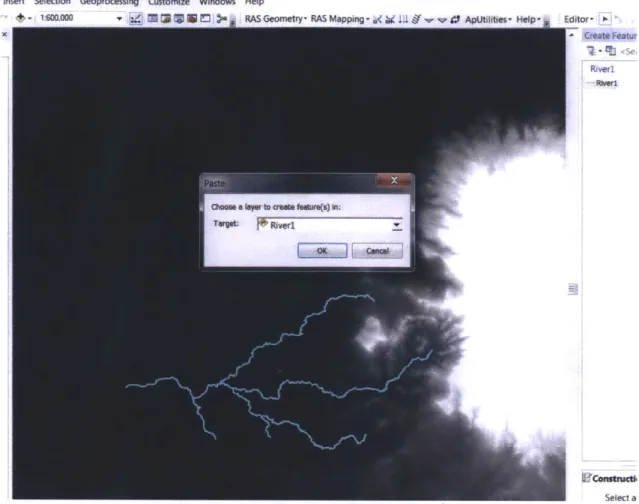
Figure 25 -Screen Shot of ArcMap: Copying Shape file feature to Stream Centerline layer... 56
Figure 26 - Screen Shot of ArcMap: Populating depth for river feature before converting it to raster ... 57
Figure 27 - Screen Shot of ArcMap: Converting river feature to raster with a cellsize of 10m... 57
Figure 28 - Screen Shot of ArcMap: Combining river raster with DEM using Raster Calculator... 58
Figure 29 - Screen shot of ArcMap: Environments specification in tools ... 58
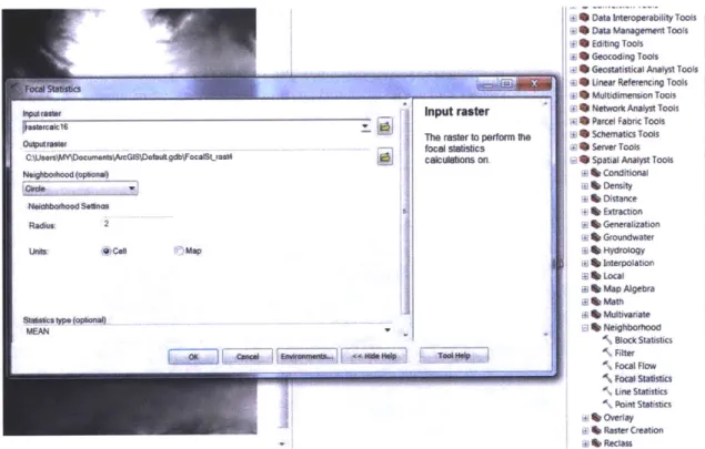
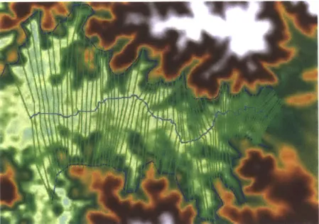
Figure 30 - Screen Shot of ArcMap: Smoothing of river cross section using focal statistics tool ... 59
Figure 31 - Screen Shot of ArcMap: Banks and Flowpaths ... 60
Figure 32 - Screen Shot of ArcMap: Stream centerline, Banks, Flowpaths and XS Cutlines...61
Figure 33 - Screen Shot of ArcM ap: RAS Layer Setup... 61
Figure 34 - Screen Shot of ArcMap: Assign line type attributes ... 62
Figure 35 - Screen Shot of ArcMap: Data export from ArcMap... 62
Figure 36 - Screen Shot of HEC-RAS: Geometric data imported as GIS format ... 63
Figure 37 - Screen Shot of HEC-RAS: M anning n table ... 64
Figure 38 - Screen Shot of HEC-RAS: Cross section data points filter ... 65
Figure 40 - Screen Shot of HEC-HMS: Summary table of w1SO for Run CNO before calibration ... 68
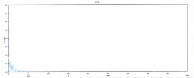
Figure 41 - Screen Shot of HEC-HMS: Precipitation loss of w150 for Run CNO before calibration ... 68
Figure 42 - Screen Shot of HEC-HMS: Soil infiltration of w150 for Run CNO... 69
Figure 43 - Screen Shot of HEC-HMS: Evapotranspiration of w150 for Run CNO ... 69
Figure 44 - Screen Shot of HEC-HMS: Optimized parameters of w150 for Run CNO... 70
Figure 45 - Screen Shot of HEC-HMS: Optimization objective function of w150 for Run CNO... 70
Figure 46 - Screen Shot of HEC-HMS: Flow graph of w150 for Run CNO after calibration ... 71
Figure 47 - Screen Shot of HEC-HMS: Flow residual of w150 for Run CNO after calibration ... 71
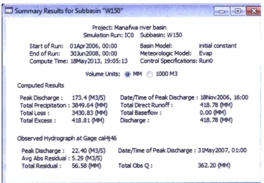
Figure 48 - Screen Shot of HEC-HMS: Flow graph of w150 for Run ICO before calibration ... 72
Figure 49 -Screen Shot of HEC-HMS: Summary table of w150 for Run ICO before calibration... 73
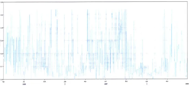
Figure 50 - Screen Shot of HEC-HMS: Evapotranspiration of w150 for Run ICO before calibration... 73
Figure 51 - Screen Shot of HEC-HMS: Soil infiltration of w150 for Run ICO before calibration ... 74
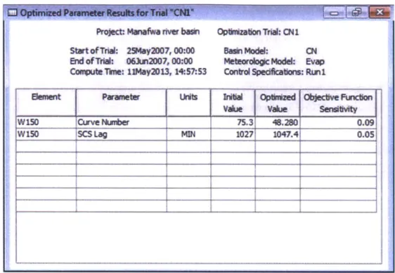
Figure 52 - Screen Shot of HEC-HMS: Cumulative precipitation loss of w150 for Run ICO before calibration ... 7 4 Figure 53 -Screen Shot of HEC-HMS: Optimization objective function of w150 for Run ICO... 75
Figure 54 - Screen Shot of HEC-HMS: Optimized parameters of w150 for Run ICO ... 75
Figure 55 - Screen Shot of HEC-HMS: Flow graph of w150 for Run ICO after calibration... 76
Figure 56 -Screen Shot of HEC-HMS: Flow graph of w150 for Run CN1 before calibration...77
Figure 57 - Screen Shot of HEC-HMS: Summary table of w150 for Run CN1 before calibration ... 78
Figure 58 -Screen Shot of HEC-HMS: Calibrated flow graph of w150 for Run CN1... 79
Figure 59 - Screen Shot of HEC-HMS: Calibration objective function of w150 for Run CN1... 79
Figure 60 - Screen Shot of HEC-HMS: Optimized parameters of w150 for Run CN1... 80
Figure 61 - Screen Shot of HEC-HMS: Potential evapotranspiration of w150 for Run CN1 after calibration81 Figure 62 - Screen Shot of HEC-HMS: Soil infiltration of w150 for Run CN1 after calibration... 81
Figure 63 - Screen Shot of HEC-HMS: Excess precipitation of w150 for Run CN1 after calibration... 82
Figure 64 - Screen Shot of HEC-HMS: flow residual of w150 for Run CN1 after calibration...82
Figure 65 - Screen Shot of HEC-HMS: Flow graph of w150 for Run IC1 before calibration ... 83
Figure 66 - Screen Shot of HEC-HMS: Summary table of w150 for Run IC1 before calibration... 83
Figure 67 - Screen Shot of HEC-HMS: Flow graph of w150 for Run IC1 after calibration ... 84
Figure 68 - Screen Shot of HEC-HMS: Summary table of wl50 for Run IC1 after calibration ... 85
Figure 69 - Screen Shot of HEC-HMS: Optimization objective function of w150 for Run ICI... 85
Figure 70 - Screen Shot of HEC-HMS: optimized parameters of w150 for Run ICI... 86
Figure 71 -Screen Shot of HEC-HMS: Flow residual of w150 for Run IC1 after calibration...86
Figure 72 - Screen Shot of HEC-HMS: Soil infiltration of w150 for Run IC1 after calibration ... 87
Figure 73 - Screen Shot of HEC-HMS: Excess precipitation of w150 for Run IC1 after calibration ... 88
Figure 74 - Screen Shot of HEC-HMS: Flow graph of w150 for RunCN2 before calibration... 88
Figure 75 - Screen Shot of HEC-HMS: Summary table of w150 for RunCN2 before calibration ... 89
Figure 76 - Screen Shot of HEC-HMS: Flow graph of w150 for RunCN2 after calibration ... 90
Figure 77 - Screen Shot of HEC-HMS: Summary table of w150 for RunCN2 after calibration... 90
Figure 78 - Screen Shot of HEC-HMS: Optimization objective function of w150 for RunCN2 ... 91
Figure 79 - Screen Shot of HEC-HMS: Optimized parameters of w150 for RunCN2... 91
Figure 80 - Screen Shot of HEC-HMS: Excess precipitation of w150 for RunCN2 after calibration... 92
Figure 82 - Screen Shot of HEC-HMS: Flow residual of w150 for RunCN2 after calibration ... 93
Figure 83 - Screen Shot of HEC-HMS: Flow graph of w150 for RunlC2 before calibration ... 94
Figure 84 - Screen Shot of HEC-HMS: Summary table of w150 for RunIC2 before calibration... 94
Figure 85 - Screen Shot of HEC-HMS: Flow graph of w150 for RunIC2 after calibration... 95
Figure 86 - Screen Shot of HEC-HMS: Summary table of w150 for RunIC2 after calibration ... 95
Figure 87 - Screen Shot of HEC-HMS: Optimization objective function of w150 for Run IC2... 96
Figure 88 - Screen Shot of HEC-HMS: Optimized parameters of w150 for Run IC2 ... 96
Figure 89 - Screen Shot of HEC-HMS: Excess precipitation of w150 for Run IC2 after calibration ... 97
Figure 90 - Screen Shot of HEC-HMS: Flow residuals of w150 for Run IC2 after calibration ... 97
Figure 91 - Screen Shot of HEC-HMS: Soil infiltration of w150 for Run IC2 after calibration ... 98
Figure 92 - Screen Shot of HEC-HMS: Flow graph of w150 for Run CN3 before calibration... 99
Figure 93 - Screen Shot of HEC-HMS: Summary table of w150 for Run CN3 before calibration ... 99
Figure 94 - Screen Shot of HEC-HMS: Flow graph of w150 for Run CN3 after calibration ... 100
Figure 95 - Screen Shot of HEC-HMS: Optimized parameter of w150 for Run CN3 ... 100
Figure 96 - Screen Shot of HEC-HMS: Summary table of w150 for Run CN3 after calibration... 101
Figure 97 - Screen Shot of HEC-HMS: Optimization objective function of w150 for Run CN3 ... 101
Figure 98 - Screen Shot of HEC-HMS: Flow residual of w150 for Run CN3 after calibration ... 102
Figure 99 - Screen Shot of HEC-HMS: Soil infiltration of w150 for Run CN3 after calibration... 102
Figure 100 - Screen Shot of HEC-HMS: Excess precipitation of w150 for Run CN3 after calibration... 103
Figure 101 - Screen Shot of HEC-HMS: Flow graph of w150 for Run IC3 before calibration ... 103
Figure 102 - Screen Shot of HEC-HMS: Summary table of w150 for Run IC3 before calibration... 104
Figure 103 - Screen Shot of HEC-HMS: Flow graph of w150 for Run IC3 after calibration ... 105
Figure 104 - Screen Shot of HEC-HMS: Summary table of w150 for Run IC3 after calibration... 105
Figure 105 - Screen Shot of HEC-HMS: Screen Shot of HEC-HMS: Optimized parameters of w150 for Run IC 3 ... 1 0 6 Figure 106 - Screen Shot of HEC-HMS: Optimization objective function of w150 for Run IC3 after ca lib ratio n ... 10 6 Figure 107 - Screen Shot of HEC-HMS: Soil infiltration of w150 for Run IC3 after calibration ... 107
Figure 108 - Screen Shot of HEC-HMS: Excess precipitation of w150 for Run IC3 after calibration ... 107
Figure 109 - Screen Shot of HEC-HMS: Flow residual of w150 for Run IC3 after calibration... 108
Figure 110 - Screen Shot of HEC-HMS: Flow graph of w150 for Run CN4 before calibration... 108
Figure 111 - Screen Shot of HEC-HMS: Summary table of w150 for Run CN4 before calibration ... 109
Figure 112 - Screen Shot of HEC-HMS: Flow graph of w150 for Run CN4 after calibration ... 110
Figure 113 - Screen Shot of HEC-HMS: Summary table of w150 for Run CN4 after calibration ... 110
Figure 114 - Screen Shot of HEC-HMS: Objective function of w150 for Run CN4 after calibration... 111
Figure 115 - Screen Shot of HEC-HMS: Optimized parameters of w150 for Run CN4... 111
Figure 116 - Screen Shot of HEC-HMS: Soil infiltration of w150 for Run CN4 after calibration... 112
Figure 117 - Screen Shot of HEC-HMS: Excess precipitation of w150 for RunCN4 after calibration... 112
Figure 118 - Screen Shot of HEC-HMS: Flow residual of w150 for Run CN4 after calibration ... 113
Figure 119 - Screen Shot of HEC-HMS: Flow graph of w150 for Run IC4 before calibration ... 114
Figure 120 - Screen Shot of HEC-HMS: Summary table of w150 for Run IC4 before calibration... 114
Figure 121 - Screen Shot of HEC-HMS: Flow graph of w150 for Run IC4 after calibration ... 115
Figure 123 - Screen Shot of HEC-HMS: Objective function of w150 for Run IC3 after calibration ... 116
Figure 124 - Screen Shot of HEC-HMS: Optimized parameters of w150 for Run IC4 ... 116
Figure 125 -Screen Shot of HEC-HMS: Excess precipitation of w150 for Run IC3 after calibration ... 117
Figure 126 - Screen Shot of HEC-HMS: Soil infiltration of w150 for Run IC3 after calibration ... 117
Figure 127 - Screen Shot of HEC-HMS: Flow residual of w150 for Run IC4 after calibration... 118
Figure 128 - Screen Shot of HEC-HMS: Flow graph of w150 for Run CN5 before calibration... 119
Figure 129 - Screen Shot of HEC-HMS: Summary table of w150 for Run CN5 before calibration ... 119
Figure 130 - Screen Shot of HEC-HMS: Flow graph of w150 for Run CN5 after calibration ... 120
Figure 131 - Screen Shot of HEC-HMS: Summary table of w150 for Run CN5 after calibration... 121
Figure 132 - Screen Shot of HEC-HMS: Objective function of w150 for Run CN5 after calibration... 121
Figure 133 - Screen Shot of HEC-HMS: Optimized parameters of w150 for Run CN5... 122
Figure 134 - Screen Shot of HEC-HMS: Soil infiltration of w150 for Run CN5 after calibration... 122
Figure 135 - Screen Shot of HEC-HMS: Excess precipitation of w150 for Run CN5 after calibration... 123
Figure 136 - Screen Shot of HEC-HMS: Flow residual of w150 for Run CN5after calibration... 123
Figure 137 -Screen Shot of HEC-HMS: Flow graph of w150 for Run IC5 before calibration ... 124
Figure 138 - Screen Shot of HEC-HMS: Summary table of w150 for Run IC5 before calibration... 124
Figure 139 - Screen Shot of HEC-HMS: Flow graph of w150 for Run IC5 after calibration ... 125
Figure 140 - Screen Shot of HEC-HMS: Summary table of w150 for Run IC5 after calibration... 125
Figure 141 - Screen Shot of HEC-HMS: Objective function of w150 for Run IC5 after calibration ... 126
Figure 142 - Screen Shot of HEC-HMS: Optimized parameters of w150 for Run IC5 ... 126
Figure 143 - Screen Shot of HEC-HMS: Flow residual of w150 for Run IC5 after calibration... 127
Figure 144 - Screen Shot of HEC-HMS: Soil infiltration of w150 for Run IC5 after calibration ... 127
Figure 145 - Screen Shot of HEC-HMS: Excess precipitation of w150 for Run IC5 after calibration ... 128
Figure 146 - Summary values histogram for performance evaluation... 130
List of Tables
Table 1 - The average of the TRMM cells contained in every sub-basin, weighted on the areas (Cecinati, 2 0 1 3 ) ... 3 0
Table 2 - Average monthly evapotranspiration value for an average year... 34
Table 3 - Recommended value for initial abstraction (HEC-1 & HEC-HIMS, 1999)... 36
Table 4 - Recommended Impervious Percentage values (HEC-1 & HEC-HIM S, 1999) ... 37
Table 5 - CN values for respective sub-basins (Bingwa, 2013)... 40
Table 6 - Parameter values for lag time estimation using Basin "n" method ... 43
Table 7 - Velocity profile measured at one location in the Manafwa River ... 44
Table 8 - Muskingum parameter estimation (R15 represents an artificial reach with length 100m) ... 45
Table 9 - SCS Soil groups and infiltration loss rates (Hydrologic Engineering Center, 2000)... 46
Table 10 - Other simulation specifications and assumptions for HEC-H MS... 47
Table 11 - Periods selected for various sim ulation runs ... 66
Table 12 - Summary of optimized parameter values for Curve Number loss method ... 128
Table 13 - Summary of optimized parameter values for Initial and Constant loss method... 129
Table 14 - Sum m ary values of objective function ... 130
Glossary
cms -cubic meter per second DEM -Digital Elevation Model DTM -Digital Terrain Model
1. INTRODUCTION
The Manafwa River basin mainly spans several districts in Eastern Uganda, namely
Bududa, Manafwa, Mbale and Butaleja. Over the years, frequent floods have posed a great
threat to the local communities. With climate change and anthropogenic perturbations
believed to have increased the flooding frequency, as many as 45,000 people are affected
each year. While Bududa is more affected by landslides caused by excessive precipitation
in rainy seasons, Manafwa, Mbale and Butaleja suffer from the runoff produced by the
upstream rainfall (Bingwa, 2013).
Figure 1- The Manafwa River Watershed (Cecinati, 2013)
The Uganda Red Cross Society (URCS) intends to design a precipitation based flood
forecasting system for the Manafwa River Basin (Figure 1). The long term goal is to have
an early flood warning system working by 2015, which would be used to assess the
end, the URCS initiated collaboration with MIT's Department of Civil and Environmental Engineering MEng team in January 2013, in an attempt to establish a hydrologic modeling system that relates upstream precipitation with downstream discharge. The team, consisting of Senior Lecturer Dr. Richard Schuhmann, and three MIT students, Francesca Cecinati, Fidele Bingwa and Ma Yan, decided to employ ArcGIS, HEC-HMS and HEC-RAS towards this goal.
The objective of this work is thus to discuss the data collection and model development, compare the performance of two loss method candidates in HEC-HMS, i.e. the Curve Number loss method, and the Initial and Constant loss method, and provide future recommendations.
2. METHODOLOGY & DATA
2.1 Overview
The objective of the modeling effort is to build a relationship between upstream
precipitation and downstream discharge on the Manafwa River. This is an essential step
in the attempt to establish an early flood warning system and to formulate a flood control
strategy.
To accomplish the objective, several software programs are chosen. As is shown in
Figure 2, HEC-HMS is employed to cakulate the discharge hydrograph at the start point of
the flood area based on historical precipitation data. HEC-RAS is then utilized to analyze
the water surface elevation, given the combination of discharge hydrograph and stream
channel geometry, in the region of interest. The stream channel geometry is provided
through ArcGIS's geo-processing capabilities, specifically with the help of HEC-GeoRAS
toolset. ArcGIS is also potentially helpful in visualizing the result generated by HEC-RAS
in 3D view.
2.2 HEC-HMS
HEC-HMS, or the Hydrologic Engineering Center - Hydrologic Modeling System, is a public-domain software that was developed by US Army Corps of Engineers. It has the capacity of simulating precipitation-runoff processes in dendritic watershed networks
(US Army Corp of Engineers). HEC-1, the antecedent version of HEC-HMS, having
originated in 1968, was the earliest research and engineering application widely employed by institutions, governments and corporations. It was based on DOS system that took input from a text file. Based on HEC-1, USACE released HEC-HMS in 1998, a version that is suitable to be operated in windows environment featuring a graphical user interface.
While HEC-HMS is versatile in many hydrologic simulations, it has limitations as well. The program is deterministic instead of stochastic, which means parameter values are fixed to be the same for every simulation neglecting probability distributions. It also assumes decoupled relationships between evapotranspiration-infiltration and infiltration-base flow. In addition, it is more suitable for dendritic river systems where diversion of flow is minimal. Looping or braided stream networks should not be simulated with HEC-HMS and its capacity to deal with back water effects is also very limited; a separate hydraulic model should be sought in dealing with these problems. Figure 3 shows a typical
Figure 3 - HEC-HMS user interface
For a HEC-HMS project, there are typically four components. They are,
1. Basin models
2. Meteorological models
3. Control specifications
4. Time series data
Basin model
A basin model incorporates the elements that physically describe the watershed
Hydrologic elements including sub-basins, reaches, junctions, reservoirs, sources and
sinks are connected in a dendritic stream network. Based on the characteristic behaviors
of these integrated elements, hydrologic computations may be carried out from upstream
sequentially (Hydrologic Engineering Center, 2005).
For this analysis, four main categories of methods are available for the user to choose from in the sub-basin editor for water losses from the sub-basin:
1. Loss methods
2. Transform methods
3. Baseflow methods
4. Routing methods
Loss Methods
Nine different loss methods can be utilized by HEC-HMS to calculate water loss volume in the sub basin from infiltration given precipitation and the physical properties of the watershed If a loss method is not selected then precipitation falling on that sub basin will not infiltrate and is considered to run off. Several of the most commonly used loss methods are described below.
The SCS Curve Number method is a simple and well-established method widely accepted for use in the US and abroad The FAO (Food and Agriculture Organization of United Nations) soil data are used to determine curve numbers. On site observations are used to estimate average percentage of impervious surface. The curve number varies as function of soil type, land use and treatment, surface condition and antecedent moisture condition
(AMC) (Hydrologic Engineering Center, 2000).
In the Green-Ampt loss method, both Darcy's Law in an unsaturated form and mass conservation are combined to describe the transport of infiltration through the soil profile and the infiltration capacity of the soil It includes an initial abstraction representing surface ponding not otherwise included in the model. Parameters can be estimated for ungauged watersheds from information about the soils present in the watershed Because the Green-Ampt model is not widely used, it is less mature (Hydrologic Engineering Center, 2000).
The continuous soil-moisture Accounting (SMA) method is a continuous model that simulates both wet and dry weather behaviors. The SMA method relies upon evapotranspiration and precipitation to calculate the behavior of water through the soil profile and into the groundwater. HEC-HMS in conjunction with SMA is able to generate basin surface runoff, groundwater flow, losses due to evapotranspiration and deep percolation over the entire basin (Hydrologic Engineering Center, 2000).
SMA is a mature model that has been used successfully in hundreds of studies throughout
the US. As a parsimonious model, it includes only a few parameters necessary to explain the variation of runoff volume. However, it is difficult to apply to ungauged areas because of a lack of direct physical relationship of the parameters with watershed properties. It may be too simple to predict losses within an event, even if it does predict total losses well (Hydrologic Engineering Center, 2000).
The initial constant loss method allows the user to specify the amount of precipitation to be infiltrated and stored within the soil before runoff begins. This water exits the water balance - i.e. it is not available for groundwater recharge or baseflow during periods of no precipitation.
Transform Methods
While loss methods allow the user to specify infiltration water losses, transform methods account for overland flow, storage and energy losses as water flows through a watershed into stream channels. Several transform methods are available for the user to select.
When the SCS Unit Hydrograph (UH) model is selected, the resulting runoff process is linear, so that greater or smaller runoff is just a multiple of the unit runoff hydrograph for
that time period (the multiple determined by the total depth of event precipitation). As a widely used empirical model to describe the relationship between direct runoff and excess precipitation, the model is based upon averages of unit hydrographs extracted from gauged rainfall and runoff for a large number of small agricultural watersheds throughout the US (Hydrologic Engineering Center, 2000).
The Kinematic-wave model is a conceptual watershed model. It represents the watershed as a broad open channel and assumes excess precipitation is the amount of flow that enters this broad open channel. The watershed runoff hydrograph is generated by solving equations that describe unsteady shallow water flow in the open channel (Hydrologic Engineering Center, 2000).
Other models include Snyder's UH model where lag, peak flow, and total time base are the most critical characteristics of the UH. A standard UH is defined and UH parameters are related to measurable watershed characteristics. In Clark's UH model, two main processes, namely translation and attenuation, are explicitly represented in the transformation of excess precipitation to runoff. Another distributed parameter model is the ModClark Model. It accounts explicitly for variations in travel time to the watershed outlet from all regions of a watershed (Hydrologic Engineering Center, 2000).
Baseflow Methods
Baseflow methods are used to represent baseflow contributions to sub-basin outflow. Baseflow values for sub-basins are not auto-calibrated by HEC-HMS. The recession method treats baseflow from a single or multiple sequential events in an exponential decay manner. It has often been used to illustrate drainage from natural storage in watersheds (Hydrologic Engineering Center, 2000). The constant monthly method is the simplest baseflow model and is efficient for continuous simulation. It represents baseflow
as a constant flow, which may vary from month to month. This baseflow is added to direct
runoff obtained from precipitation to calculate total discharge in the simulation
(Hydrologic Engineering Center, 2000). The linear reservoir method addresses mass
conservation by routing infiltrated precipitation to the channel. It is used in conjunction
with the continuous soil-moisture (SMA) model and "simulates storage and movement of
subsurface flow as storage and movement of water through reservoirs" (Hydrologic Engineering Center, 2000).
Routing Methods
Routing methods are used to simulate flows in open channels. The modified Puls routing
method, also called storage routing or level-pool routing, is achieved through both a finite
difference approximation of the continuity equation and an empirical description of
momentum conservation (Hydrologic Engineering Center, 2000). Like the modified Puls
model, the Muskingum routing method utilizes a simple finite difference approximation
of the continuity equation. Reach storage is represented by the sum of prism storage and
wedge storage (Hydrologic Engineering Center, 2000). Also based on a simple finite
difference approximation of the continuity equation and simplification of the momentum
equation, the Kinematic-wave model represents a watershed as two angled plane
surfaces. The water flows over each surface until it reaches the channel at the
intersection of the planes. Looking at a cross section, the shape of the watershed appears
like an open book. Stream channels would follow the book's center binding. Although the
Kinematic-wave model is mainly used to represent overland flow on the plane surfaces, it
is also instrumental in simulating channel flow (Hydrologic Engineering Center, 2000).
The simplest routing model in HEC-HMS is the Lag Model The outflow hydrograph is
identical to the inflow hydrograph except that the latter leads by a specific duration. In the
Lag Model, the flows are not attenuated, which means no shape change is present in the
results could be duplicated with other models by carefully choosing parameter values (Hydrologic Engineering Center, 2000).
Meteorological Model
The second major component of HEC-HMS is the meteorological sub-model. The meteorological sub-model is where time series data and storm rainfall depths are assigned to sub-basins in the watershed in the Basin Model for various storms. HEC-HMS treats the hydrologic response of any watershed as driven by rainfall and evaporation over the watershed
Precipitation could be any of the following kind: (1) observed rainfall from historic event; (2) frequency-based hypothetical rainfall event; (3) maximum possible precipitation event at a given location. Historical rainfall data are helpful in calibration and verification of model parameters. Hypothetical or design storms are used if the accuracy of the model must be checked, when modeling extreme precipitation events, or if a risk of flooding must be assessed Similarly, both observed historical data and hypothetical data can be used for evapotranspiration.
The Meteorological model includes four different methods for historical precipitation analysis (Hydrologic Engineering Center, 2005):
1. Precipitation data analyzed outside the program are represented by the user-specified hyetograph method
2. Both recording and non-recording gauge data are represented by the gage weights method
3. Dynamic data problems are addressed by the inverse distance method 4. Radar rainfall data are utilized with the gridded precipitation method
The frequency storm method produces balanced storms given specific exceedance probability using statistical data. Regulations for precipitation are implemented to estimate standard project flood in the standard storm method. The SCS hypothetical storm method is based on Natural Resources Conservation Service criteria and implements primary precipitation distributions for design analysis.
Control Specifications
The Control Specifications component enables the user to specify the simulation start time, end time, and the time interval. Multiple control specifications can be created and connected to simulation runs so that when any time control specification is changed, the correspondent simulation period will change accordingly.
Time Series Data
The Time Series Data component integrates input data related to time into the simulation. These data include precipitation, and observed flow. In the model, the precipitation data are in the form of a DSS file, whereas observed flows are manually tabulated.
2.3 HEC-RAS
HEC-RAS, or Hydrologic Engineering Center - River Analysis System, is an integrated system designed to perform one-dimensional hydraulic calculations for networks with natural and constructed channels (US Army Corp of Engineers, 2008).
HEC-RAS is comprised of four major constituents for one-dimensional river analysis.
1. Steady flow water surface profile calculations. 2. Unsteady flow simulations.
3. Movable boundary sediment transport simulations. 4. Water quality analysis.
The four components share a common geometric data representation and common geometric and hydraulic simulation routines (US Army Corp of Engineers, 2008).
Steady flow means that at any point, depth and velocity remains constant with respect to time, such as a constant head discharge in a long straight canal The steady flow water surface profiles calculations are useful in determining water surface profiles with steady as well as gradually changed flow. In this context, the system is capable of dealing with not only a single river reach, but also dendritic systems and a full network of stream channels. Flow regimes including subcritical, supercritical as well as mixed are all within the capacity of the system. The computational procedures comply with the fundamental energy equations in one-dimensional form. In the case that the water surface profile is dramatically changed, the momentum equation is employed This includes hydraulic jumps, bridges and stream junctions. Energy losses are addressed by the Manning's equation (friction), and contraction/expansion. The computations take into account the effect of various elements of the stream network like bridges, culverts, weirs, and spillways. The steady system is mainly used for flood plain management and flood insurance studies to assess floodway encroachment. The steady system approach is also applied in the evaluation of impacts of channel improvement (US Army Corp of Engineers, 2008).
Unsteady flow means depth and/or velocity changes in magnitude or direction with respect to time; a flood hydrograph or a curve in a channel are examples of unsteady flow. The unsteady simulation component was developed primarily for subcritical flow regime simulations. It enables simulation of one-dimensional unsteady flow in a full network of open channels. It also has the capacity to carry out hydraulic calculations similar to that of the steady flow component for cross-sections, culverts, bridges, etc. In addition, water storage areas and hydraulic connections between them could also be modeled The two fundamental principles in this context are the principle of mass conservation and the
principle of momentum conservation (US Army Corp of Engineers, 2008). Theories behind these calculations that are embedded in HEC-RAS system are detailed in HEC-RAS Reference Manual (US Army Corp of Engineers, 2008).
The main objective of the HEC-RAS model is to determine water surface elevations at locations of interest. This can be achieved either by the user inputting a set of flow data, for the steady flow scenario, or through hydrograph routing, for the unsteady flow scenario. Data needed to perform the necessary calculations varies among geometric data, steady flow data, or unsteady flow data. The geometric data are needed for any type of analysis (US Army Corp of Engineers, 2008).
2.4 HEC-GeoRAS
HEC-GeoRAS is an ArcGIS extension software program developed collaboratively by HEC (Hydrologic Engineering Center) and ESRI (Environmental Systems Research Institute, Inc.). HEC-RAS continues to be developed and the latest version is version 4. The current version of the software is the result of the effort by HEC and ESRI to transplant the functionality of GeoRAS 3.1 to the ArcGIS platform.
As a set of tools specially designed to handle geospatial data for connection with HEC-RAS, the extension enables users with rudimentary experience with GIS to create HEC-RAS input files from DTMs (Digital Terrain Model) and complementary data sets. It is also useful in viewing and processing exported results from HEC-RAS (US Army Corp of Engineers, 2009).
DTM files of a river system in TIN (triangulated irregular network) or GRID format are used to create the import file for HEC-RAS in HEC-GeoRAS. A series of point, line and polygon layers are created. The RAS layers include Stream Centerline, Flow Path
Centerlines, Main Channel Banks, and Cross Section Cut Lines. Additional geometric data can be extracted by using additional RAS layers including Land Use, Levee Alignments, Ineffective Flow Areas, Blocked Obstructions, Bridges/Culverts, Inline Structures, Lateral Structures and Storage Areas (US Army Corp of Engineers, 2009). The process flow of using HEC-GeoRAS is illustrated in Figure 4 below.
F
3. MODEL DEVELOPMENT
3.1 HEC-HMS Analysis
3.1.1 Watershed delineation & Geometry file Creation
The watershed is delineated in the ArcGIS environment. A Shape file is used to generate a
basin model that is then directly used by HEC-HMS.
3.1.2 Precipitation Data Acquisition
Rain gauges are usually the best source for historical rainfall data. However, in the study
area in Uganda, the availability of rain gauges is limited. Three rain gauges are identified
in different regions. While the Bududa and Buginyanya gauges are more recent, the
Tororo data spans over the years 1929 to 1986 (Cecinati, 2013).
At the same time, a range of satellite precipitation data was retrieved Among these data,
the TRMM-3B42 performs best in the Mt. Elgon region. Compared with ground rain
gauges, the TRMM data appear to be more reliable and consistent than Bududa and Buginyanya gauge data. While Tororo data are also considerably consistent, the time
interval of one year is too coarse for the modeling purpose in the short term (Cecinati,
2013).
In order for HEC-HMS to utilize the TRMM rainfall data, weighted averages are taken with
respect to the area of each sub basin underlying each data cell Overlaying the TRMM file
onto the watershed shape file, the values of precipitation for every sub-basin were
calculated A map of the sub-basins identified with TRMM cells appears in Figure 5 and
Table 1 contains equations used to calculate weightings for each sub-basin based upon
Figure 5 -The sub-basins identified with TRMM cells (Cecinati, 2013) Sub-basin Equation W120 2/3 B + 1/3 C W130 3/7 E + 4/7 B W140 1/21 D + 2/21 A + 3/21 E + 15/21 B W150 1/3 E + 1/3 F + 1/3 C W160 1/8 A + 7/8 D W170 D W180 1/2 D + 1/2 E W190 1/15 D + 14/15 E W200 2/3 D + 1/3 E W210 1/2 E + 1/2 F W220 E
Table 1 - The average of the TRMM cells contained in every sub-basin, weighted on the areas (Cecinati, 2013)
The mathematical operation is repeated for each sub-basin for each day to give a record of daily rainfall estimates for every sub basin, which is then used in HEC-HMS. The calculated rainfall data is presented in Appendix A. More details can be found in Cecinati's
3.1.3 Observed Flow Acquisition
The Ministry of Water and Environment in Uganda has been managing one river stage gauge in Busiu, which is a community near the center of the watershed (Figure 6). The
river gauge is located beside a bridge linking Mbale and Manafwa districts (Figure 7).
Figure 6 - River gauge position inside the Manafwa River watershed (Cecinati, 2013)
250 - - - -- - -
-200
-E
50
0
Figure 8 - Water level of the Manafwa River in Busiu, as recorded in elevation above the gauge by the Water Resources Department from March 1997 - March 2008
The river gauge provides river stage data dating from March 1997 to June 2008, except for the period between November 1997 and June 1999 (Figure 8). The missing data are believed to be attributed to a flood in 1997.
To understand the geometric properties of the Manafwa River, and to verify available data, measurements of the river cross section were taken at two different locations during a site visit. One location was selected to be in a bending section of the river, whereas the other was in the straight part, recognizing the difference in the geometry (Figure 9).
.Mam
Figure 9 - River cross sections position (Cecinati, 2013)
In Figure 9, the cross section on the left is in a river curve, downstream; the cross section
on the right is in a straight section, upstream.
River Cross Section Distance (m)
5 10
River Cross Section Distance (m)
0 5 0 -20 =40 60 80
Figure 10 - Plot of river cross sections
In Figure 10, the cross section on the Ieft is in the river curve at a meandering region
(river flow into cross section), whereas the cross section on the right is in a straight
segment. Based on the comparison between river gauge recording and the cross section
measurement, the river stage data appears consistent and reasonable.
0 0 20 -C 40 060 80 10
-7-3.1.4 Evapotranspiration Estimation
In short term hydrologic modeling, such as flood event modeling, the effect of evapotranspiration can be safely omitted However, when the period of simulation increases to as long as a year, evapotranspiration is significant in the water budget.
At the present stage of this project, the Monthly Average method is chosen in Meteorological Models. With regard to evapotranspiration rates in Central and Eastern Africa, sources differ on the monthly average value. While Dagg et al. (1970) claimed that annual values of potential evaporation rates ranged from 1800 to 2200 mm annually, and average monthly values seldom fell below 90 mm, the average monthly evaporation values over the years are shown to be considerably lower in the map provided by Centre for Ecology & Hydrology, which appear in Table 2. For current long term modeling purpose, the monthly average evaporation values are estimated from the map retrieved online (Centre for Ecology & Hydrology).
Month Average Monthly Evaporation (mm/month)
Low High Average
Jan 70 90 80 Feb 70 90 80 Mar 70 100 85 Apr 70 100 85 May 60 90 75 Jun 40 70 55 Jul 40 70 55 Aug 50 70 60 Sep 60 100 80 Oct 50 110 80 Nov 60 100 80 Dec 50 100 75
Table 2 - Average monthly evapotranspiration value for an average year (Centre for Ecology & Hydrology)
coefficient is also required. Although the watershed is home to a variety of plantations, the coefficient is estimated to be 1.05 as is tabulated for rice and maize in the FAO Corporate Document Repository (Natural Resources Management and Environment Department).
3.1.5 SCS CN Number Method
The Loss Method chosen for HEC-HMS modeling is the SCS Curve Number (CN) method. It is a well-established method with relatively high accessibility. The method incorporates land use, land cover and soil type information into three parameters, namely initial abstraction, CN, and impervious area percentage. Each sub-basin has its own set of parameters specified respectively.
Typically, three mechanisms contribute to the abstraction for a single storm event (1)
rainfall interception, (2) depression storage, and (3) infiltration into the soil (Patel, 2009).
These three elements are incorporated into the term Initial Abstraction, which is a
threshold value which when exceeded by precipitation results in runoff (HEC-1 &
HEC-HMS, 1999). As is illustrated in Figure 11 below, the dark area represents the initial
abstraction Ia. It can be considered as the water loss before the runoff begins. In contrast,
F stands for the actual retention after runoff begins.
Rainfall (P)
Runoff
(Q)
F
Initial
Time
abstraction la
Infiltratioi
curve
The initial loss, or initial abstraction, is not a mandatory parameter. While it is recommended that the initial abstraction value range from 0 mm to 1 mm, as seen below in Table 3, it is a common practice to relate initial abstraction (i.e. the amount of water infiltrated before runoff begins) to the potential maximum retention (i.e. the maximum amount of water that will be absorbed after runoff begins). The ratio of initial abstraction to potential maximum retention is commonly quoted as 0.2 (The Shodor
Education Foundation, Inc., 1998).
Land Use Recommended Initial Abstraction (mm)
Paved Areas 0
Sloped Roofs 0
Flat Roofs 0
Lawn Grass 0.75
Open Fields with Minimal Vegetation 0.5
Open Fields with Cover Crop 0.75
Wooded Areas
Table 3 - Recommended value for initial abstraction (HEC-1 & HEC-HMS, 1999)
For this project, the value of the initial abstraction is set to blank as a start and is changed only for calibration purposes, because the flow result is calibrated against actual flow data where antecedent moisture has been taken into account. Another consideration is that losses to depression storage and canopy are neglected and evapotranspiration data are specified separately.
The impervious area percentage accounts for the fact that certain parts of the modeled area are not a good media for water to infiltrate, such as rooftops, pavements etc. No infiltration losses are incurred from this impervious fraction of the sub basins. In Table 4, recommended values for the impervious area percentage are listed. As the watershed is
most accurately described as open space and is minimally paved, the impervious area
parameter value is estimated to be 1% (HEC-1 & HEC-HMS, 1999).
Land Use Type
Highways, Parking Areas 95
Commercial, Industrial, Office
Apartments, Condominiums
Single Family Residential (including duplex or split lot housing) 1-10 units/acre Parks 85-95 70-80 5-60 5 - 10
Open Space (fields, wooded area) 1 -5
Table 4 - Recommended Impervious Percentage values (HEC-1 & HEC-HMS, 1999)
Figure 12 - Manafwa watershed Sub basins (Bingwa, 2013)
Figure 12 shows the different sub-basins with name codes used in HEC-HMS illustrated in different colors. The FAO (Food and Agriculture Organization) developed a map of land use through their AFRICOVER program in 2009, which serves as the main source of information on land use in this project (Figure 13). Soil data were also obtained from FAO's Harmonized World Soil Database (HWSD) represented in different soil clay content as shown in Figure 14.
Lad Use Code
*10495-3782-W7 [:110613-W8 Ek 10769-12634(3)[Z10] -110789-12634(3)Z10] 2l028M E 20326-3011 G 20326-3012 El 20389-3012 Q20391-3719 :J21677 El3043-S0308 ED 40371 E] 42178-Ri EJ42347-R1 E15003-9
Percent Clay Content 21 023 024 30 31 32 ,40 --'49 & 54
Figure 14 - Soil data - percent clay content, from HWSD database (Bingwa, 2013)
Using Matlab, land cover data and soil type data are processed and mapped The result is a
CN map as shown in Figure 15.
100
The CN value in one particular sub basin is obtained by averaging the CN readings within that sub-basin utilizing a statistics function in ArcMap. The result is tabulated below in Table 5. Sub-basin Mean CN W120 75.6 W130 78.0 W140 71.4 W150 75.3 W160 83.2 W170 82.4 W180 86.4 W190 82.2 W200 77.4 W210 77.7 W220 80.2
Table 5 - CN values for respective sub-basins (Bingwa, 2013)
The major disadvantages of the SCS CN method are fixing the initial abstraction ratio, and lack of clear guidance on how to vary Antecedent Moisture Conditions (AMC) (Patel,
2009). More information can be found in Bingwa's (2013) work.
3.1.6 Estimating Sub basin Lag Time
The sub basin-specific lag time is a representation of the time from the center of mass of precipitation excess to the peak discharge (Stantec consulting Inc., 2009). Many equations have been proposed to estimate basin lag time over the last century. Among them, Snyder's equation is most frequently cited (Loukas & Quick, 1996). US Army Corps of Engineers (USACE) customized Snyder's equation, introducing N values relating the effect of development on lag time. The USACE equation appears in the following form (Boucher, 2011).
ag=24xNx( S.5")038
ag is the elapsed time from the beginning of an assumed continuous series of unit effective rainfalls over an area to the instant at which the rate of the resulting runoff at the area concentration point equals 50 percent of the maximum potential rate of the resulting runoff at that point. L is the length of the main drainage path in miles. Lea is
the length along the drainage path from a point opposite the centroid of the watershed to the outlet point in miles. S is the overall slope of the main watercourse in feet per mile.
Nis the dimensionless weighted watershed Manning coefficient (Boucher, 2011).
In the Drainage Manual by the City and County of Sacramento, a similar method called Basin "n" Method is presented, and is easier to implement than USACE's equation (Boucher, 2011). The Basin "n" lag equation was revised by the USACE and the U.S. Bureau of Reclamation based on Snyder's equation. It appears in the form below.
Lg =Cxn x(L x) 033
Lg is the lag time in seconds. C is a constant with value of 174 when lag time is calculated
in seconds. n is the tabulated Basin "n" overbank channelization roughness value for developed and undeveloped scenarios. The table of n values is attached in the Appendix B.
L is the length of the longest watercourse measured as approximately 90% of the distance from the point of interest to the headwater divide of the basin. It is measured in meters when lag time is in seconds. e is the length of the longest watercourse measured upstream from the point of interest to a point close to the centroid of the basin. It is also measured in meters when lag time is in seconds. S is the overall slope of the longest watercourse between the headwaters and concentration point. It is measured in meter per meter when lag time is in seconds (City and County of Sacramento, 1996).
a- ast
n seaon GeoCeuang CAtofmi Wndoam elp
* OWmIm -. A
Them we
Ircfne 3 5 5: 12644130911 8 4 19 12644130911 001028 1075 1062
Fgr1-ce Sto Arcap: De22 trni ofmI p0 1ag 10e7q'u
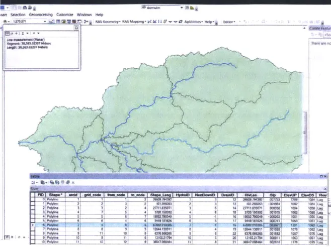
Figure 16 - Screen Shot of ArcMap: Determination of lag equation parameters
As shown in Figure 16 above, ArcGIS is utilized to obtain values for L, Lc, and S in the equation above. L is obtained from the shape length column in the attribute table in
L.
ArcGIS. L is measured from the outlet of each sub basin to the centroid of the sub basin. S is obtained from slope column in the attribute table. The parameters and lag times for this project are determined and presented in Table 6.
Parameters for lag equation Sub-basin C n L (m) L, (m) S (mm) Lg (hr) w120 174 0.12 26509.79 13163 0.007733 8.5 w130 174 0.12 401.2851 8376 0.019 1.6 w140 174 0.12 27711.84 12995 0.000938 12.2 w150 174 0.12 67082.21 30363 0.003861 17.1 w160 174 0.12 19082.79 9723 0.000578 10.6 w170 174 0.12 9449.182 4421 0.000741 6.2 w180 174 0.12 3720.15 3468 0.001075 4.0 w190 174 0.12 12644.13 6985 0.001028 7.6 w200 174 0.12 13165.22 12044 0.000911 9.4 w210 174 0.12 36547.1 21913 0.002818 13.3 w220 174 0.12 6376.866 9787 0.001882 6.1
Table 6 - Parameter values for lag time estimation using Basin "n" method
Another method to calculate Lag Time based on estimation of concentration time can be found in the HEC technical reference manual (Hydrologic Engineering Center, 2000).
3.1.7 Estimating Reach Routing Parameters
Reach routing represents the movement of water through stream channels (Bras, 1990).
A discharge hydrograph is generated through routing based on channel properties and
the inflow hydrograph. Two routing models are considered in this project.
The simplest routing model in HEC-HMS is the Lag Model However, it neglects attenuation in the routing processes. As mentioned earlier, the Muskingum routing method utilizes a simple finite difference approximation of continuity equation. It is chosen as it better represents the attenuation of the hydrograph. The method requires two parameters, i.e. K and x. More details of the method can be found in Bras's (1990) work. The Muskingum K value is essentially the time needed for water to travel through a
certain reach. The lengths of all reaches are obtained using ArcGIS.
Field measurements were taken of flow velocity profiles at the location where cross sections were measured on the Manafwa River; these results appear in Table 7 below.
Depth (ft.) Velocity (cm/s) 0 54 0.5 50 1 54 1.5 54 2 48 2.2 28
Table 7 - Velocity profile measured at one location in the Manafwa River
The measured surface velocity of the Manafwa River is around 0.5 m/s. Considering the
velocity upstream of this point may have equal or higher surface velocities because upstream channels would have steeper slopes and narrower cross sections , the reaches upstream are conservatively assigned an average velocity of 0.5 m/s in estimating the Muskingum K value. The reaches in the middle of the basin are assigned a velocity of 0.4 m/s, whereas the last segment of reach is assigned a velocity of 0.3 m/s. The result is
Parameters
Sub-basin River Average Velocity Muskingum L (i) (m/s) K (hr) w120 R12 26509.79 0.5 14.7 w130 R13 401.2851 0.5 0.2 w140 R30 27711.84 0.4 19.2 w150 R15 100 0.5 0.1 w160 R50 19082.79 0.3 17.7 w170 R60 9449.182 0.4 -6.6 w180 R40 3720.15 0.4 2.6 w190 R80 12644.13 0.4 8.8 w200 R20 13165.22 0.4 9.1 w210 R21 36547.1 0.5 20.3 w220 R22 6376.866 0.5 3.5
Table 8 - Muskingum parameter estimation (R15 represents an artificial reach with length 100m) One thing to note here is the length of reach R15; it is set to a small arbitrary value of 100 m. The reason is discussed in the calibration section below.
3.1.8 Initial and Constant Loss method parameters
Three parameters are required in the Initial and Constant loss model: (1) impervious percentage, (2) initial loss, and (3) constant loss rate. As discussed in the curve number method, impervious percentage is assumed to be 1% throughout the watershed The initial loss represents interception and depression storage and is not unlike the initial abstraction in the curve number method The value of the initial loss is set to be 0 as simulation results are calibrated against day-to-day observed flow data.
The constant loss rate represents the maximum potential rate of precipitation loss, and is assumed to be constant throughout each event. Recommended values can be found in the technical reference manual (Hydrologic Engineering Center, 2000) and are presented