Master's Theses (2009 -) Dissertations, Theses, and Professional Projects
Passenger Car Equivalent Factors for Level Freeway
Segments Operating under Moderate and
Congested Conditions
Umama Ahmed Marquette University
Recommended Citation
Ahmed, Umama, "Passenger Car Equivalent Factors for Level Freeway Segments Operating under Moderate and Congested Conditions" (2010).Master's Theses (2009 -).Paper 60.
PASSENGER CAR EQUIVALENT FACTORS FOR LEVEL FREEWAY SEGMENTS OPERATING UNDER MODERATE AND
CONGESTED CONDITIONS
by
Umama Ahmed
A Thesis Submitted to the faculty of the Graduate School, Marquette University,
in Partial Fulfillment of the Requirements for the Degree of Master of Science
Milwaukee, Wisconsin August 2010
ABSTRACT
PASSENGER CAR EQUIVALENT FACTORS FOR LEVEL FREEWAY SEGMENTS OPERATING UNDER MODERATE AND
CONGESTED CONDITIONS
Umama Ahmed Marquette University, 2010
The significant impact Heavy Vehicles (HV) have on freeway operations has been identified since the first edition of the Highway Capacity Manual (HCM). The method of incorporating their impact in freeway capacity calculations has changed through the years. The HCM 2000 used Passenger Car Equivalent (PCE) values and percent of trucks/buses and Recreational Vehicles (RV) to account for HV effect on capacity. However PCE values in the most recent HCM edition rely on a limited field database and extensive simulation runs based on this information; they were calibrated on ‗steady-flow‘ traffic operations. The objective of this effort was to indentify and quantify HV characteristics that have an impact of freeway throughput at various congestion levels on level, urban freeways using 1.2 million individual vehicle observations, with an emphasis on operations at LOS E and F. It was desired to use the products of this effort as recommended inputs for future simulation runs of congested freeway flow conditions. Passenger Car (PC) and HV headways were found to increase with HV presence in the traffic stream. A similar pattern was found for the PCE factor. The PCE value, under congested conditions and more than 9% HV presence, was found to be 1.76, which is higher than the HCM 2000-recommended value of 1.5 for level freeway sections. Also, passenger car was found to have the effect of more than 1 PC at congested condition with high HV presence.
ACKNOWLEDGEMENTS
Umama Ahmed
I would like to show my gratitude to my supervisor, Dr. Alexander G. Drakopoulos, for his encouragement and support, which enabled me to complete my thesis. I also appreciate the guidance given me by the members of my advisory committee: Professor David A. Kuemmel and Richard C. Coakley, P.E. My final acknowledgement is owed to my husband Mostafa Z. Uddin; and my parents: Faruque Ahmed and Nurjahan Begum, for their understanding, endless patience and encouragement when it was most required.
TABLE OF CONTENTS ACKNOWLEDGEMENTS ... i TABLE OF CONTENTS ... ii LIST OF TABLES ... iv LIST OF FIGURES ... vi CHAPTER 1. INTRODUCTION ... 1
1.1Highway capacity, Heavy Vehicles and Passenger Car Equivalent (PCE) value ... 1
1.2 Research Objective ... 3
1.3 Thesis Layout ... 4
CHAPTER 2.LITERATURE REVIEW ... 5
2.1 Historical Review of Development of PCE ... 5
2.2 Methods of Estimating PCE ... 6
2.3 Relation with LOS ... 8
2.4 Effect of Heavy Vehicles ... 13
CHAPTER 3.METHODOLOGY ... 18
3.1 Passenger Car Equivalent Factor Calculation Method ... 18
3.2 Regression Analysis ... 18
3.3 Analysis of Variance (ANOVA) ... 19
3.4 Headway Measurement ... 19
TABLE OF CONTENTS (Continued)
CHAPTER 4. AVAILABLE DATA ... 22
4.1 Data Collection Site ... 22
4.2 Data Collection System Description ... 22
4.3 Data Description ... 22
CHAPTER 5. DATA ANALYSIS ... 27
5.1 Introduction ... 27
5.2 General Study Site Traffic Flow Characteristics ... 27
5.3 Free Flow Speed ... 31
5.4Headway Relation with Speed ... 34
5.5 Heavy Vehicle Effect on Lighter Vehicles ... 37
5.5.1 Lagging Passenger Car Headways ... 37
5.5.2 Passenger Car-Heavy Vehicle Pair Headways ... 45
5.5.3 Gross Vehicle Weight-Headway Relation ... 50
5.6 Heavy Vehicle Percentage and PCE Factor Relationship ... 54
CHAPTER 6. CONCLUSIONS AND RECOMMENDATIONS ... 67
6.1 Conclusions ... 67
6.2 Recommendations for Future Research ... 70
LIST OF TABLES
Table 2.1 Estimates of PCE values for Trucks on Level Freeway Segments
from Krammes et al. Study ... 9
Table 2.2 Effect of Traffic Flow Rate on PCE at Level Grades found from Webster et al. Study ... 9
Table 2.3 Summary of PCE and Capacity values found for Al-Kaisy et al. Study ... 12
Table 2.4 Mean Headway for different Leading-Lagging Vehicle Combination found at Tanaboriboon et al. Study ... 15
Table 2.5 Mean Headway for different Leading-Lagging Vehicle Combination found at Krammes et al. Study ... 16
Table 3.1 Average gross vehicle weight for all vehicles present in the field data set ... 21
Table 4.1 Number of vehicle observations by date and by lane ... 26
Table 5.1 Frequency of vehicles observed in the study site ... 28
Table 5.2 Regression model summary of Headway vs. Vehicle speed ... 36
Table 5.3 ANOVA results for Headway vs. Vehicle Speed regression analysis ... 36
Table 5.4 Coefficient values for the Headway vs. Vehicle Speed equation ... 36
Table 5.5 Types of Lagging-Leading pairs with lagging Passenger Car and their frequencies in the dataset ... 41
Table 5.6 Headway-Speed relationship for vehicle pairs with Lagging Passenger Cars ... 42
Table 5.7 Types of Lagging-Leading vehicle pairs with Lagging Passenger Cars ... 43
Table 5.8 Average value and the 95% Confidence Interval of Headway (seconds) for different Passenger Car- Semi Truck lagging-leading pair ... 47
LIST OF TABLES (Continued)
Table 5.10 Passenger Car Equivalent factor relation with heavy vehicle percentage in the traffic stream ... 64
LIST OF FIGURES
Figure 3.1 FHWA Classification of vehicles ... 20
Figure 4.1 Data Collection Site ... 24
Figure 4.2 Central Processing Unit in the controller cabinet ... 25
Figure 4.3 Pavement-embedded detectors, saw cuts and pull box visible ... 25
Figure 5.1 Weekday hourly traffic distribution ... 29
Figure 5.2 Weekend hourly traffic distribution ... 30
Figure 5.3 Vehicle Speed-Volume curve for the study site ... 32
Figure 5.4 Average Headway relationship with Vehicle Speed ... 35
Figure 5.5 95% mean Headway Confidence Intervals for Lagging-Leading vehicle pairs with Lagging Passenger cars within specific speed ranges ... 44
Figure 5.695% mean Headway Confidence Intervals for Passenger car- following-Truck class 8 and Truck class 8-following- Passenger car within specific speed ranges ... 48
Figure 5.7 95% mean Headway Confidence Intervals for Passenger car- following-Truck class 9 and Truck class 9-following- Passenger car within specific speed ranges ... 49
Figure 5.8 95% mean Headway Confidence Intervals for Gross Vehicle Weight categories within specific speed ranges ... 53
Figure 5.9 Speed-volume and LOS relationships-all vehicles ... 57
Figure 5.10 Speed-volume and LOS relationships-passenger cars only ... 58
Figure 5.11 Speed-volume and LOS relationships-trucks present- up to 3% trucks ... 59
Figure 5.12 Speed-volume and LOS relationships - 3% to 6% trucks ... 60
Figure 5.13 Speed-volume and LOS relationships- 6% to 9% trucks ... 61
LIST OF FIGURES (Continued)
Figure 5.15 Heavy Vehicle PCE vs. Heavy Vehicle percentage in the
traffic stream ... 65 Figure 5.16 Passenger Car PCE vs. Heavy Vehicle percentage in the
CHAPTER 1. INTRODUCTION
1.1 Highway capacity, Heavy Vehicles and Passenger Car Equivalent (PCE) Values
Highway capacity is the maximum hourly rate at which vehicles can reasonably be expected to traverse a point or a uniform section or lane of a roadway during a given time period under prevailing roadway and traffic conditions (1). It is expressed in passenger cars per hour per lane. The presence of large vehicles (Heavy Vehicles-HV) in the traffic stream results in a reduction in capacity. The reduction is due to the adverse effect of HV on traffic-stream performance. The following HV attributes that adversely impact capacity have been addressed in past research efforts:
1. HV are larger than Passenger Cars (PC), and thus take up more space in the traffic stream;
2. HV have operating capabilities (acceleration/deceleration) that are inferior to those of PC, thus requiring longer headways; and,
3. Drivers of nearby vehicles keep longer headways from HV.
To account for the adverse impact of HV present in a traffic stream in highway capacity analysis, traffic volumes containing a mix of vehicle types are typically converted into an equivalent flow of PC using Passenger Car Equivalents (PCEs). The procedure in the Highway Capacity Manual (HCM) allows freeway traffic volumes containing a mix of vehicle types and measured in vehicles per hour (vph) to be converted by the use of a HV factor, fHV, into an
heavy vehicle adjustment factor has historically been based on separate PCE for trucks, buses, and Recreational Vehicles (RVs). The HCM 2000 (2) defines the heavy vehicle adjustment factor as:
𝑓𝐻𝑉 = 1+𝑃 1
𝑡 𝐸𝑡−1 +𝑃𝑟 𝐸𝑟−1 1.1
Where, Et, Er = PCE for trucks/buses and recreational vehicles (RVs) in the traffic stream,
respectively;
Pt, Pr = Proportion of trucks/buses and RVs in the traffic stream, respectively;
fHV = HV adjustment factor.
The HCM 2000 considered identical PCE values for both buses and trucks, assuming that there is no difference in their performance on freeways and multilane freeways.
Since the 1965 version of HCM, separate PCE values for HV were provided for level, rolling and mountainous terrain freeway segments. Level terrain has been defined as the ―type of terrain that includes short grades of no more than 2 percent.‖ In the HCM 2000, PCE for level freeway segments are considered to be 1.5 and 1.7 for Trucks and RVs respectively. These PCE values were calculated considering a steady-state flow condition. PCE values were independent of the level of service (LOS) prevailing on the freeway segment. However, under steady-state flow conditions, the effect of HV on traffic flow can reasonably be expected to vary with prevailing traffic level due to the interaction between HV and smaller vehicles in the traffic stream. At low volumes, when drivers have relative freedom to choose their speeds, it is reasonable to expect that larger vehicles would have only a small effect on traffic flow. As congestion level increases, the HV effect can be expected to increase due to a greater
interaction between vehicles in the traffic mix and reduced opportunities for drivers to pass slower-moving vehicles.
1.2 Research Objective
The significant impact HV have on freeway operations has been identified since the first edition of the HCM. The method of incorporating their impact in freeway capacity calculations has changed through the years. The HCM 2000 used PCE values and percent of trucks/buses and RV to account for HV effect on capacity. However PCE values in the most recent HCM edition rely on a limited field database and extensive simulation runs based on this information; they were calibrated on ‗steady-flow‘ traffic operations.
The present effort investigates the effect of HV presence with a focus on congested and forced-flow conditions which are of major importance to practicing traffic engineers dealing with urban freeways facing recurrent congestion, freeway work zone- or traffic incident-caused congestion on a daily basis.
An extensive vehicle classification database that provided information about 1.2 million individual vehicles was used to analyze HV behavior on a level urban basic freeway section.
The objective of this effort was to indentify and quantify HV characteristics that have an impact on freeway throughput at various congestion levels, with an emphasis on operations at LOS E and F. It was desired to use the products of this effort as recommended inputs for future simulation runs specifically calibrated to replicate forced-flow conditions.
information collected under congested and severely congested conditions.
HV impacts were to primarily be assessed through investigations of the relations of HV headways with truck percentage in the traffic stream, gross vehicle weight and type of lagging-leading vehicle class combinations.
1.3 Thesis layout
Chapter 2 is a literature review of previous studies related to the effects of HV on freeway traffic flow and the development of PCE factors, including the description of the basis on which the HCM PCE factors were developed. The chapter contains a presentation of previous efforts on relationships between PCE and LOS; and HV effect on traffic flow. Chapter 3 states the methodology used to analyze the research hypotheses. Chapter 4 describes the study site and data collection procedure. A description of field data is also provided in this chapter. Chapter 5 is the data analysis chapter, which contains results on the research hypotheses. Chapter 6 presents the conclusions and recommendations drawn from the results of this research.
CHAPTER 2. LITERATURE REVIEW
This section includes the historical review of the Passenger Car Equivalent (PCE) concept for Heavy Vehicles (HV) on level freeway segments and describes different methods used to calculate PCE. Also the relationship of PCE with Level of Service (LOS) is discussed here. Previous research efforts on HV effect on traffic movement are also briefly stated in this chapter.
2.1 Historical review of development of PCE
The 1950 Highway Capacity Manual (HCM) introduced the estimate that, on two-lane highways on level terrain, trucks have the same effect as two Passenger Cars (PC). That HCM edition intimated that this estimate was based on the number of passenger cars passing trucks compared to the number of passenger cars passing passenger cars.
The 1965 HCM formally introduced both the Level of Service (LOS) concept and the term Passenger Car Equivalent (PCE). LOS was defined in terms of two parameters: operating speed and volume-to-capacity ratio. PCE for heavy vehicles was defined as ―The number of passenger cars displaced in the traffic flow by a truck or a bus, under prevailing roadway and traffic conditions.‖ For two-lane highways, PCE was calculated considering different LOS. But for multilane highways operating under LOS B through LOS E, a constant PCE value of 2 was suggested for trucks. This was due to the fact that PCE values research in that area had been restricted principally to operation at or near LOS B; rationalized values for LOS E were developed, adapted from LOS B values by means of limited field data obtained during operation at capacity. The 1965 HCM
suggested that further research was needed on PCE values for different LOS on multilane highways.
The 1985 HCM also related PCE with LOS for two-lane highways but for multilane level freeways a single value of 1.7 for trucks for all LOS was recommended.
The current 2000 HCM also uses a single PCE of 1.5 for level freeways, regardless of LOS. The currently suggested PCE value is based on the effect of HV dimensions and performance under steady-state traffic flow conditions.
2.2 Methods of Estimating PCE
Several approaches to estimate PCE values have been used. The most commonly applied approaches are as follows:
1. The constant volume-to-capacity ratio approach; 2. The equal-density approach; and,
3. The headway approach.
The constant volume-to-capacity ratio approach was developed based on the output of a multilane freeway simulation model developed at the Midwest Research Institute. PCE values were based on mixed traffic volumes that consumed the same proportion of roadway capacity (produced the same volume-to-capacity ratio) as PC-only volumes (3). The constant volume-volume-to-capacity ratio approach was appropriate for calculating PCEs when LOS was a consideration for PCE calculation. But it is not applicable to the current procedure, which estimates PCE only under a steady-state condition (4).
traffic) when they operated at equal densities (measured in vehicle/mile) was used to determine PCE values. The practicality of PCE values based on this method was debated, since traffic streams operating at different speeds must have different degrees of freedom to maneuver. Thus it was suggested that the basis for equivalence of two traffic streams should not be equal density, but rather densities that feel the same to the driver in terms of proximity to other vehicles and freedom to maneuver (4).
The headway (time between successive vehicles in the traffic stream) approach uses actual measurements of the relative position maintained by drivers in the traffic stream under prevailing conditions to arrive at PCE values. The basic formula of PCE using the headway approach is as follows:
𝑃𝐶𝐸 =ℎ𝑡
ℎ𝑐 2.1
Where, ht= Average headway (in seconds) maintained by trucks following PC; and,
hc = saturation flow headway of PC following PC.
This equation takes into account the effect of larger truck size and lower truck acceleration characteristics; truck drivers are expected to keep longer headways than PC following PC, thus PCE values are expected to be greater than 1 (5).
Two factors which affect PCE magnitude have traditionally been considered in PCE estimation: HV length and HV operating capabilities. Trucks, take up more space than PC; therefore headways for PC following trucks will be longer than those for PC following PC- the numerator of equation 2.1 will be larger than the denominator, increasing with truck length. In addition, inferior truck operating capabilities (lower acceleration rates and lower travel speeds)
compared to PC require truck drivers to maintain longer headways from leading vehicles than PC drivers maintain, contributing to a large numerator in equation
2.1.
Ideally the numerator and denominator of equation 2.1 are based on actual field observations. Field measurements include the effects of both above-mentioned factors and maybe other factors as well that are yet to be identified.
Krammes et al. (4) analyzed a mixed traffic stream and developed an equation considering headway differences between trucks and other vehicles, as shown below:
𝑃𝐶𝐸 = 𝐼−𝑝 ℎ𝑝𝑡+ℎℎ𝑡𝑝−ℎ𝑝𝑝 +𝑝ℎ𝑡𝑡
𝑝𝑝 2.2
Where, p = percentage of trucks at a mixed traffic stream;
hpt = Mean headway time in seconds for trucks following PC; htp = Mean headway time in seconds for PC following trucks;
hpp = Mean headway time in seconds for PC following PC;
htt = Mean headway time in seconds for trucks following trucks.
Krammes et al. (4) recommended equation 2.2 as the final formulation for use in highway capacity analysis instead of equation 2.1 because it accounts separately (and thus more accurately) for the impact of trucks leading or following PC or other trucks.
2.3 Relation with LOS
Krammes et al (4) analyzed data collected from six-lane, basic level freeway segments on the Kingery Expressway in Chicago and on the La Porte Freeway in Houston. Lagging time headways were measured for four combinations of pairs of PC and trucks in a mixed traffic stream. The four
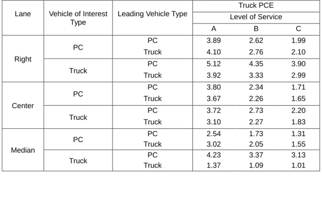
combinations were: PC following a PC, PC following a truck, truck following another truck, and a truck following a PC. The mean lagging headway time was estimated using an analysis of covariance model. The model was calibrated with a range of flow rates from approximately 400 to 1,300 vehicles per hour per lane. To avoid extrapolation beyond the limits of the data, predicted values were estimated only for flow rates and speeds that approximated the upper traffic density limits of LOS A, B, and C. PCE values for trucks were computed using the mean headway, proportion of trucks in each lane and LOS. The results indicated that PCE values (based on equation 2.2) increased as LOS decreased from A to C. However, they suggested more work on their suggested PCE calculation method and did not recommend their results as conclusive findings. Table 2.1 shows the estimated PCE values for each LOS and each lane found from the study. It also shows the overall PCE value for all lanes combined for each LOS. This overall value is a weighted average of the value for each lane, weighted according to the distributions of trucks by lane at each LOS.
Webster et al. (6) did a study to find the effect of traffic flow rate on PCE for basic level freeway sections using the FRESIM simulation model.PCEs were calculated for five truck types having differing weight-to-power ratios and overall lengths. The five truck types examined were: semi-trailer with five axles, single unit truck with two axles, semi-trailer with four axles, double trailer truck with five axles, and triple trailer truck. Flow rates tested were at 500, 1000, 1500 and 2000 vphpl. Table 2.2 shows the resulting PCE values for the five subject truck types examined. The study results indicated that, PCE is sensitive to traffic flow
rate at level grades, and that, in general, PCE increases with traffic flow rate.
TABLE 2.1 Estimates of PCE values for Trucks on Level Freeway Segments from Krammes et al. Study (4).
Lane Vehicle of Interest
Type
Leading Vehicle Type
Truck PCE Level of Service A B C Right PC PC 3.89 2.62 1.99 Truck 4.10 2.76 2.10 Truck PC 5.12 4.35 3.90 Truck 3.92 3.33 2.99 Center PC PC 3.80 2.34 1.71 Truck 3.67 2.26 1.65 Truck PC 3.72 2.73 2.20 Truck 3.10 2.27 1.83 Median PC PC 2.54 1.73 1.31 Truck 3.02 2.05 1.55 Truck PC 4.23 3.37 3.13 Truck 1.37 1.09 1.01
TABLE 2.2Effect of Traffic Flow Rate on PCE at Level Grades found from Webster et al. Study (6).
Traffic flow rate (vphpl)
PCE
Semi-trailer with five axles
Single unit truck with two
axles
Semi-trailer with four axles
Double trailer truck with five
axles Triple trailer truck 500 1.02 1.03 1.09 1.02 1.02 1000 1.05 1.05 1.04 1.06 1.07 1500 1.14 1.07 1.06 1.12 1.16 2000 1.42 1.04 1.15 1.42 1.62
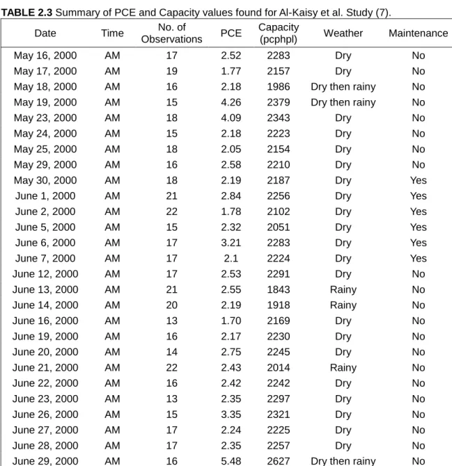
Al-Kaisy et al. (7) hypothesized that the effect of HV on freeway traffic is greater when the facility is operating at oversaturated conditions than when it is operating at undersaturated (below-capacity) conditions. That hypothesis was based on the fact that during congestion or stop-and-go conditions, the acceleration and deceleration cycles, are expected to impose an extra limitation on the performance of HV, and that may affect the PCE value. The data were collected from a level freeway segment with 3 lanes in one direction during the morning peak hours (7:30 to 9:30 am). Congestion was due to heavy commuter traffic during that time period. A total of 27 data sets, each containing several 5-min vehicle observations, comprising more than 38 hours of capacity observations were collected using video recording. Table 2.3 shows the summary of PCE factors and the mean capacity that resulted from individual optimization runs for that site.
The PCE factors ranged from 1.70 to 5.48 (see Table 2.3). The PCE value greater than 4.00 was found in three data sets where the weather became rainy midway of the count. The authors suggested a few reasons why these days should not be considered as valid. Typically at that site, PC counts used to decrease and HV counts used to increase as time progressed at the morning. In those three days, the decrease in PC counts should have been attributed to two factors; the increase in HV counts and the rainy weather. Optimization simply attributed all the reduction in PC counts to the increase in HV counts and therefore the PCE factors were overestimated. Neglecting those data sets and considering the remaining ones, a mean PCE value of 2.36 was found. This
value is considerably higher than the corresponding PCE factor of 1.5 recommended by the HCM 2000 which was calculated for traffic under steady-state conditions. Therefore, the research hypothesis that the PCE value for HV during oversaturated conditions is higher than the PCE value during free flow condition was validated. In light of this finding, the authors recommended the use of a more realistic PCE factor for HV for calculating queue discharge flow capacity (7).
TABLE 2.3 Summary of PCE and Capacity values found for Al-Kaisy et al. Study (7).
Date Time No. of
Observations PCE
Capacity
(pcphpl) Weather Maintenance
May 16, 2000 AM 17 2.52 2283 Dry No
May 17, 2000 AM 19 1.77 2157 Dry No
May 18, 2000 AM 16 2.18 1986 Dry then rainy No
May 19, 2000 AM 15 4.26 2379 Dry then rainy No
May 23, 2000 AM 18 4.09 2343 Dry No
May 24, 2000 AM 15 2.18 2223 Dry No
May 25, 2000 AM 18 2.05 2154 Dry No
May 29, 2000 AM 16 2.58 2210 Dry No
May 30, 2000 AM 18 2.19 2187 Dry Yes
June 1, 2000 AM 21 2.84 2256 Dry Yes
June 2, 2000 AM 22 1.78 2102 Dry Yes
June 5, 2000 AM 15 2.32 2051 Dry Yes
June 6, 2000 AM 17 3.21 2283 Dry Yes
June 7, 2000 AM 17 2.1 2224 Dry Yes
June 12, 2000 AM 17 2.53 2291 Dry No June 13, 2000 AM 21 2.55 1843 Rainy No June 14, 2000 AM 20 2.19 1918 Rainy No June 16, 2000 AM 13 1.70 2169 Dry No June 19, 2000 AM 16 2.17 2230 Dry No June 20, 2000 AM 14 2.75 2245 Dry No June 21, 2000 AM 22 2.43 2014 Rainy No June 22, 2000 AM 16 2.42 2242 Dry No June 23, 2000 AM 13 2.35 2297 Dry No June 26, 2000 AM 15 3.35 2321 Dry No June 27, 2000 AM 17 2.24 2225 Dry No June 28, 2000 AM 17 2.35 2257 Dry No
The Institute for Research study (8) produced a set of PCE values for a broad range of vehicle types on urban level freeways under five hourly volume levels (0-599 vphpl, 600-999 vphpl, 1000-1499 vphpl, 1500-1799 vphpl and 1800-2000+ vphpl). For Single-unit trucks and buses, PCE values ranged from 1.1 at 0-599 vphpl to 1.6 at 1800-2000+ vphpl volume level. For Tractor Trailers PCE values found to be 1.1 at 0-599 vphpl to 2.0 at 1800-2000+ vphpl. PCE was calculated based on 5 minute flow. The results indicated that PCE values varied based on volume levels, increasing with increasing volume. This finding agreed with the findings of Webster et al. (6). However Roess et al. (3) concluded that the idea of varying PCE for varying volume level would be a vexing one. Their logic behind the conclusion was that, the adoption of PCE values varying with volume would present serious problems in capacity analysis procedures, greatly complicating computations. Because the design benefits of smaller PCEs at low volumes would be minimal, they recommended that constant PCEs with volume should be used for vehicle types on level terrain; however, they did not provide a specific suggestion about which PCE value at which volume should be used.
2.4 Effect of heavy vehicles
To examine the effect of heavy vehicles on the movement of a mixed traffic stream, Sarvi (9) observed the behavior of 240 vehicles in which 120 were HV-following-PC, and 120 were PC-following-PC and PC-following-HV under congested traffic conditions. Each vehicle-following case was analyzed in microscopic detail over a length of 700 meters over which the speed and position of each vehicle were identified. Results indicated that there was a significant
difference in the vehicle-following behavior of HV compared to that of PC. HV drivers were found to keep longer headways and spacings when following other vehicles. PC drivers were found to travel further behind HV (in terms of headway and spacing) than when following other PC. Also, PC-following-HV headways were found to be longer than HV-following-PC headways. Based on these results, the author concluded that, there was a significant difference in the vehicle-following behavior of HV; also the presence of a HV in a leading position in the traffic stream had a significant negative effect on the headways kept by trailing vehicles (resulted in longer headways by trailing drivers).
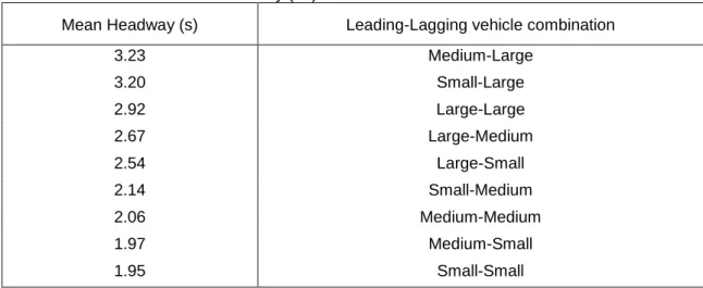
Y. Tanaboriboon et al. (10) conducted research to evaluate the effect of vehicle size on highway capacity in Thailand. The headway for 5 min and 15 min flow was collected when the freeway section was at or near its capacity (LOS E). Headway data were obtained from a mixed traffic stream as well as a traffic stream containing only small vehicles due to imposed HV restrictions. The researchers observed that the proportion of HV in a traffic lane affected the average headways of all types of vehicles. Comparisons of headways kept between pairs of vehicles for different vehicle pair types indicated the following:
i. Headways involving small vehicles with medium-sized vehicles, taken as a group, were significantly shorter than those involving HV with the two other sizes (small and medium) and with each other.
ii. Headways involving HV following medium-sized or small vehicles were not significantly different from each other.
prevailing traffic conditions was capacity reduction on the order of 15%. The authors concluded that their findings impact should be taken into consideration for PCE calculations. Table 2.4 shows the headway data collected for different leading-following vehicle combinations.
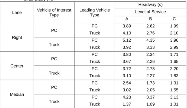
Similar results were obtained in a study by Krammes et al. (4). Headway data were obtained from a field dataset with flow rates ranging from 400 to 1,300 vehicles per hour per lane which approximated conditions of LOS A, B and C. It was found that, 95 percent of the time, PC maintained slightly higher headway and spacing when traveling behind HV than PC. Also, it was observed from the headway data that, vehicle headways decreased with increasing congestion level (see Table 2.5).
TABLE 2.4 Mean Headway for different Leading-Lagging Vehicle Combination found at Tanaboriboon et al. Study (10).
Mean Headway (s) Leading-Lagging vehicle combination
3.23 Medium-Large 3.20 Small-Large 2.92 Large-Large 2.67 Large-Medium 2.54 Large-Small 2.14 Small-Medium 2.06 Medium-Medium 1.97 Medium-Small 1.95 Small-Small
TABLE 2.5 Mean Headway for different Leading-Lagging Vehicle Combination found at Krammes et al. Study (4).
Lane Vehicle of Interest
Type Leading Vehicle Type Headway (s) Level of Service A B C Right PC PC 3.89 2.62 1.99 Truck 4.10 2.76 2.10 Truck PC 5.12 4.35 3.90 Truck 3.92 3.33 2.99 Center PC PC 3.80 2.34 1.71 Truck 3.67 2.26 1.65 Truck PC 3.72 2.73 2.20 Truck 3.10 2.27 1.83 Median PC PC 2.54 1.73 1.31 Truck 3.02 2.05 1.55 Truck PC 4.23 3.37 3.13 Truck 1.37 1.09 1.01
There were several differences of the studies by Tanaboriboon et al. (10) and Krammes et al. (4):
I. Data for two studies were collected from two different continents; one from Asia and another from North America.
II. Data for the study by Tanaboriboon et al. (10) were collected when the freeway section was at capacity (LOS E), whereas data for the study by Krammes et al. (4) were collected during free-flow conditions (LOS A to C).
Despite these differences, the Tanaboriboon et al. and Krammes et al. studies provided some important insights of vehicle headway behavior with changing congestion level:
congestion level.
II. Headway decreases with increasing congestion level (headway decreases with decreasing LOS).
III. Drivers of all vehicles keep the longest headways under free-flow conditions and the shortest headways at forced-flow conditions.
CHAPTER 3. METHODOLOGY 3.1 Passenger Car Equivalent Factor Calculation Method
Among the methods that have been used to calculate the Passenger Car Equivalent factor (PCE), the headway ratio method based on the following equation was used in the present effort:
𝑃𝐶𝐸 = 𝐻𝑉 ℎ𝑒𝑎𝑑𝑤𝑎𝑦𝑃𝐶 ℎ𝑒𝑎𝑑𝑤𝑎𝑦 3.1
The numerator of equation 3.1 is the Heavy Vehicle (HV) headway measured
under a given set of traffic flow conditions; the denominator is the measured Passenger Car (PC) headway at capacity, measured in a PC-only traffic stream. Thus the HV effect on the traffic stream under a given set of traffic flow conditions is represented by the additional time consumed by the HV present in the traffic stream.
3.2 Regression Analysis
A regression analysis was performed using the Statistical Package for the Social Sciences (SPSS) software in order to evaluate the fit of various models (equations) to the relationship of headway (dependent variable) with average speed (fixed factor). The best-fitting equation among a set of eleven tested models (linear, quadratic, cubic, logarithmic, inverse, power, compound, S, logistic, growth and exponential) was chosen for presentation in this thesis.
3.3 Analysis of Variance (ANOVA)
Analysis of Variance using the SPSS software package was used extensively in order to establish general descriptive headway statistics as well as the 95% Confidence Intervals (95% CI) for mean headway values. Detailed explanations on the use of ANOVA results are provided in section 5.5.1.
3.4 Headway Measurement
The difference between the time at which the front axle of the leading vehicle and the front axle of the trailing vehicle crossed the detector loop was considered as the trailing vehicle‘s headway for this research. Headway was measured in seconds. Headways calculated in this manner for individual vehicles were cross-checked using the relationship between hourly volume and headway.
3.5 Vehicle Classification
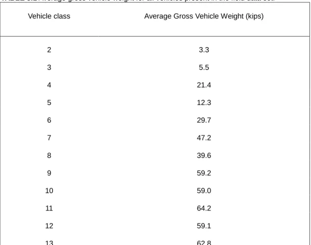
Vehicles in the field data set for this thesis had been classified according to the Federal Highway Administration (FHWA) classification. FHWA classifies vehicles into 13 classes; vehicles within classes greater than 3 would be defined as heavy vehicles for Highway Capacity Manual purposes. Figure 3.1 shows the FHWA vehicle classification. Table 3.1 presents the average gross vehicle weight of each vehicle class present in the field data.
FIGURE 3.1. FHWA Classification of vehicles. (Source: FHWA Traffic Monitoring Guide)
TABLE 3.1 Average gross vehicle weight for all vehicles present in the field data set.
Vehicle class Average Gross Vehicle Weight (kips)
2 3.3 3 5.5 4 21.4 5 12.3 6 29.7 7 47.2 8 39.6 9 59.2 10 59.0 11 64.2 12 59.1 13 62.8
CHAPTER 4. AVAILABLE DATA 4.1 Data Collection Site
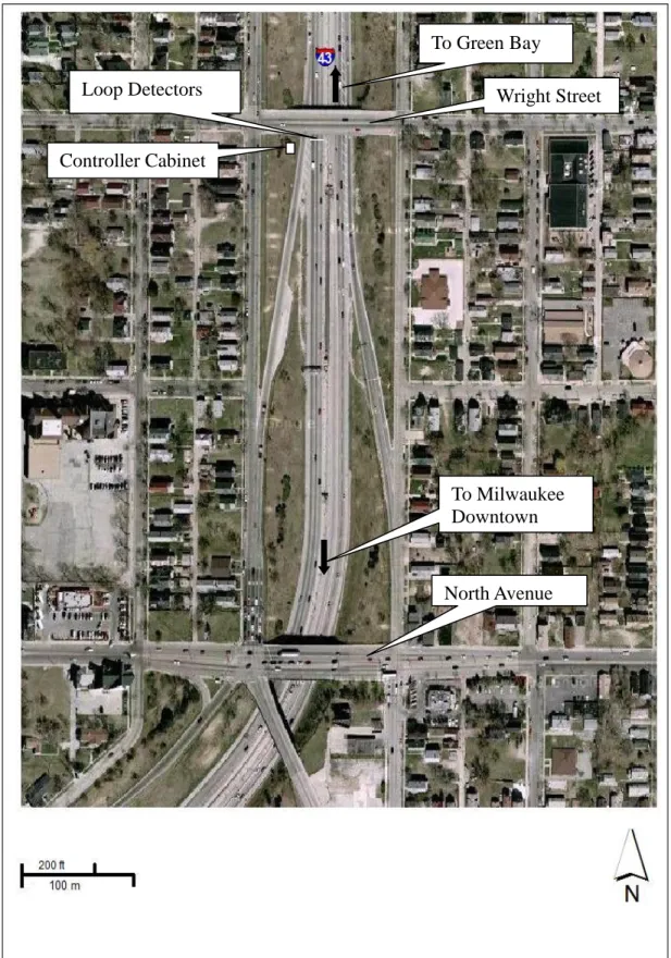
The present analysis is based on field data collected in the southbound direction of a six-lane section of Interstate 43 located just North of downtown Milwaukee, Wisconsin (population 630,000). The data collection site (see Figure 4.1) was preceded by an 8,000 ft straight and level section with 12 ft lanes and 12 ft shoulders on both sides. The section speed limit was 55 mph; it dropped to 50 mph 1,000 ft upstream of the detector location. On-and off-ramps were present at regular intervals of approximately 0.75 mile. Data were collected through detectors placed immediately South of the Wright Street overpass (see Figure 4.1) in each of the three southbound lanes.
4.2Data Collection System Description
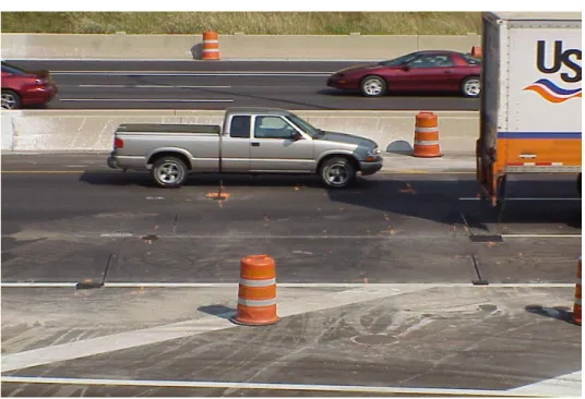
The installed data collection system consisted of a controller cabinet containing the Central Processing Unit (CPU) (Figure 4.2), connected to pavement-embedded detector arrangements (Figure 4.3). Separate detector sets were placed within each lane of travel. Each set consisted of two loop detectors with a piezo-electric vehicle weight sensor between them. Detector signals were sent to the CPU for processing and storage.
4.3 Data Description
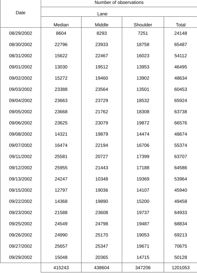
Field data were collected for a total of twenty-one days between August 29, 2002 and September 29, 2002 (see Table 4.1). The raw data consisted of the date and time at which the vehicle crossed the detectors, the FHWA vehicle
class, vehicle length in feet, speed in mph, number of axles, individual axle weight, vehicle wheelbase(s) and the lane in which the vehicle was traveling.
A total of 1,201,053 vehicles were counted during the study period; 415,243 vehicles traveled in the median lane, 438,604 vehicles in the middle lane and 347,206 in the shoulder lane (see Table 4.1). Data were analyzed using the Statistical Package for Social Sciences (SPSS) software.
FIGURE 4.1. Data Collection Site. Wright Street North Avenue Loop Detectors Controller Cabinet To Green Bay To Milwaukee Downtown
FIGURE 4.2. Central Processing Unit in the controller cabinet.
TABLE 4.1Number of vehicle observations by date and by lane.
Date
Number of observations
Lane
Median Middle Shoulder Total
08/29/2002 8604 8293 7251 24148 08/30/2002 22796 23933 18758 65487 08/31/2002 15622 22467 16023 54112 09/01/2002 13030 19512 13953 46495 09/02/2002 15272 19460 13902 48634 09/03/2002 23388 23564 13501 60453 09/04/2002 23663 23729 18532 65924 09/05/2002 23668 21762 18308 63738 09/06/2002 23625 23079 19872 66576 09/08/2002 14321 19879 14474 48674 09/07/2002 16474 22194 16706 55374 09/11/2002 25581 20727 17399 63707 09/12/2002 25955 21443 17188 64586 09/13/2002 24247 10348 19369 53964 09/15/2002 12797 19036 14107 45940 09/22/2002 14368 19890 15200 49458 09/23/2002 21588 23608 19737 64933 09/25/2002 24549 24798 19487 68834 09/26/2002 24990 25170 19053 69213 09/27/2002 25657 25347 19671 70675 09/29/2002 15048 20365 14715 50128 415243 438604 347206 1201053
CHAPTER 5. DATA ANALYSIS 5.1 Introduction
The present chapter contains the findings of this research effort. General database information is presented first, in order to establish relationships between the fundamental traffic flow parameters at the study location (volume, speed, density, free flow speed, peaking characteristics, traffic mix, and number of trucks throughout the day). This is accomplished through general descriptive statistics (frequencies and means) tables and graphs (bar charts, histograms).
Subsequently the analysis focus shifts to testing a number of hypotheses set to examine Heavy Vehicle (HV) influence on freeway traffic operations. A major part of this effort is focused on headways of individual and lagging-leading pairs of vehicles, and the relationship of this variable with other traffic flow parameters, such as speed, volume, truck presence (percent of trucks) and vehicle weight.
5.2 General Study Site Traffic Flow Characteristics
A total of 1,201,053 vehicles were observed during the study period, of which 84.8% were passenger cars (PC) and 9.0% were light trucks. Among heavy vehicles, single-trailer trucks with five axles (vehicle class 9-see Figure 3.1) were the most prevalent at 1.7% and single-trailer trucks with four or less axles (vehicle class 8-see Figure 3.1) were 1.6% of the total vehicle counts. Table 5.1 shows the frequency of each vehicle type in the total vehicle observations.
was 70,675 vehicles per day in all three lanes together. Weekday peak hours of traffic were observed generally between 6 am to 9 am and again from 3 pm to 6 pm. During weekends, peak traffic was observed between 11 am and 7 pm. Figures 5.1 and 5.2 stacked bar histograms present weekday and weekend hourly traffic patterns with light vehicles (classes 2 and 3) shown in blue and heavy vehicles (classes 4 and above) shown in green.
TABLE 5.1 Frequencies of vehicles observed at the study site.
FHWA
class
Frequency Percent Valid
Percent
Cumulative Percent
Motorcycle 1 3,427 .3 .3 .3
PC 2 1,018,981 84.8 84.8 85.1
Four-tire single-unit truck 3 108,584 9.0 9.0 94.2
Buses 4 9,011 .8 .8 94.9
Two-axle, six-tire single-unit truck 5 13,953 1.2 1.2 96.1
Three-axle, single-unit truck 6 6,187 .5 .5 96.6
Four-or-more- axle, single-unit truck 7 290 .0 .0 96.6
Four-or-less axle, single-unit trailer 8 19,694 1.6 1.6 98.3
Five-axle, single trailer 9 20,467 1.7 1.7 100.0
Six-or-more-axle, single trailer 10 91 .0 .0 100.0
Five-or-less-axle, multi-trailer 11 301 .0 .0 100.0
Six-axle, multi-trailer 12 67 .0 .0 100.0
Seven-or-more-axle, multi-trailer 13 2 .0 .0 100.0
29
30
5.3 Free Flow Speed
According to the HCM 2000, Free-Flow Speed (FFS) is the mean speed of passenger cars measured during low to moderate flows (up to 1,300 pc/h/ln). This average PC speed reflects the net effect of all prevailing geometric conditions, such as lane width, lateral clearance, interchange density, number of lanes, speed limit and vertical and horizontal alignment that influence speed. The HCM 2000 indicates that speed data that include PC and HV can be used to determine FFS for level terrain or moderate downgrades but should not be used for rolling or mountainous terrain (2). As the data for this research was collected from a level freeway segment, the FFS was determined for the mixed traffic stream containing both PC and HV. Figure 5.3 shows the Speed-Volume curve developed for the study site.
32
The Speed-Volume curve was developed using hourly per-lane volumes based on average 15-minute flows and the corresponding 15-min average speeds of the mixed traffic stream.
The ―rays‖ (straight lines converging at the origin) of Figure 5.3 indicate the boundaries between Levels of Service (LOS), segregating the collected data into distinct ―sectors‖ for each LOS. Visual inspection reveals that, as congestion levels increase (moving from left-to-right) in Figure 5.3, average speeds start decreasing within LOS C at about 1,200 vphpl.
In order to adhere to the HCM FFS definition intent (the average speed measured at low to moderate flows), speed observations corresponding to flows less than or equal to 1200 vphpl were selected and their average value (61 mph) was considered to be the study location‘s FFS (see horizontal line at 61 mph).
The capacity of the study location (based on the highest 15-minute measured flows) was determined to be approximately 2,500 vphpl.
5.4 Headway Relation with Speed
To examine the vehicle headway relation with speed, individual vehicle speeds were divided into 10 speed ranges: 0-10 mph, 10-15 mph, 15-20 mph, 20-25 mph, 25-30 mph, 30-35 mph, 35-40 mph, 40-45 mph, 45-50 mph and greater than 50 mph. The mean headway for each of these speed ranges was calculated. A strong relationship between mean vehicle headway and vehicle speed was identified (r = 0.981 – see Table 5.2). It was found that headway decreased with an increase in vehicle speed and reached its minimum value at a range of 40-45 mph; above 45 mph, headway started increasing with increasing speed. Thus it was documented that the analyzed freeway section reached its capacity (coincident with minimum headways) within the range of 40-45 mph. Figure 5.4 shows average headway relationship with speed.
A regression analysis using average headway as the dependent and speed range as the independent variable had an excellent fit at the 0.000 level of significance (Table 5.3) when a Quadratic equation was fit to the data (see coefficients on Table 5.4 – all regression model coefficients were significant at the 0.000 level). The relation can be expressed by the following equation:
𝑉𝑒ℎ𝑖𝑐𝑙𝑒 𝐻𝑒𝑎𝑑𝑤𝑎𝑦 = 0.0018 ∗ 𝑆𝑝𝑒𝑒𝑑2+ −0.14 ∗ 𝑆𝑝𝑒𝑒𝑑 + 4.94 5.1 Where, Vehicle Headway was measured in seconds.
35
TABLE 5.2 Regression model summary of Headway vs. Vehicle speed.
R R Square Adjusted R Square Std. Error of the Estimate
.981 .962 .951 .149
TABLE 5.3 ANOVA results for Headway vs. Vehicle Speed regression analysis.
Sum of Squares df Mean Square F Sig.
Regression 3.947 2 1.973 88.787 .000
Residual .156 7 .022
Total 4.102 9
TABLE 5.4 Coefficient values for the Headway vs. Vehicle Speed equation.
Unstandardized Coefficients Standardized
Coefficients t Sig.
B Std. Error Beta
Speed -.140 .015 -3.152 -9.443 .000
Speed ** 2 0.0018 .000 2.383 7.137 .000
5.5 Heavy Vehicle Effect on Lighter Vehicles
A total of 1,200,992 lag-lead vehicle pair observations were available from field data. Enough observations for analysis purposes were available for vehicle pairs involving PC (FHWA class 2), four-tire single-unit trucks (FHWA class 3), four-or-less-axle single-trailer trucks (FHWA class 8) and five-axle single-trailer trucks (FHWA class 9).
A primary hypothesis of this research was that the presence of HV in mixed traffic stream had a negative impact on freeway capacity. This hypothesis was addressed in the present effort in a number of ways, focusing primarily on the effects HV had on headways.
5.5.1 Lagging PC Headways
Previous research efforts determined differences in the headways maintained between specific pairs of vehicle classes. Typically, lighter vehicles were found to maintain larger headways when following (lagging) heavier vehicles than when following other lighter vehicles (4). This finding was tested herein with the available field data. For this effort, lighter vehicles in the database were paired with their leading vehicles. It was desired to test the hypothesis that lighter vehicles would keep longer headways when following a heavier vehicle, than when following another lighter vehicle.
Among the available light vehicle-following-light vehicle pairs, ―PC-following-PC‖ (FHWA vehicle class 2) and ―PC-following-four-tire single-unit truck‖ (FHWA Truck class 3) had a significant presence in the traffic stream.
Among light vehicle-following-heavier vehicle pairs, only ―PC-following-four-or-less-axle, single-trailer truck‖ (FHWA Truck class 8) and ―PC-following-five axle, single-trailer truck‖ (FHWA Truck class 9) pairs had significant numbers of observations for analysis. Table 5.5 shows major lagging-leading vehicle pairs with a lagging PC and the corresponding frequencies.
It was shown earlier that a strong relationship exists between average headway and speed. It was desired to investigate whether headway-speed relationships between particular vehicle class pairs followed this general trend, and whether statistically significant differences existed in headways maintained between particular vehicle classes. The same speed ranges used in section 5.4 to investigate the headway-speed relationship, 0-10 mph, 10-15 mph, 15-20 mph, 20-25 mph, 25-30 mph, 30-35 mph, 35-40 mph, 40-45 mph, 45-50 mph and greater than 50 mph, were used in the present lagging-leading vehicle pair headway investigation, as well. Due to an absence of sufficient observations for PC following trucks class 8 or 9, the speed range 0-10 mph was excluded from the analysis. Only headways equal to or shorter than 10 seconds were included since longer headways are not typically due to vehicle interactions, but, rather, random arrivals under very low volume conditions. Also for speed range 10-15 mph, PC-following-Truck class 9 had only 28 observations. This number was insufficient to provide a representative result for actual field conditions.
An analysis of Variance (ANOVA) of headway (dependent variable) versus Lagging-Leading pair (fixed factor) for each of the ten analyzed speed ranges was used in this investigation. Descriptive statistics, statistical significance and
95% Confidence Intervals (95% CI) for average headway values are shown in Tables 5.6 and 5.7. The 95% headway CI for each vehicle pair type at each analyzed speed range is presented graphically in Figure 5.5.
Table 5.6 shows general headway descriptive statistics for headways maintained between particular vehicle pairs; for example, the average headways between two PC for the speed range of 15-20 mph was 2.65 seconds. The 95% CI for that value was 2.62-2.68 seconds. The average headway for a PC following a truck class 9 within the same speed range was 4.61 seconds with a 95% CI 4.39 to 4.82 seconds. Since the two 95% CI for these two types of Lagging-Leading vehicle pairs did not overlap, the average headway lagging PC maintained from leading trucks class 9 was statistically significantly larger than the average headway they maintained from leading PC at the 95% confidence level.
This same comparison is shown in Table 5.7 for these two vehicle type pairs. In this case headway differences between a Lagging-Leading PC-PC (column (I) Lagging-Leading vehicle pair) and a Lagging-Leading PC-truck class 9 pair (column (J) Lagging-Leading vehicle pair) is shown in column Mean Difference (I-J). In the above example, for the 15-20 mph speed range, the value -1.95 seconds corresponds to the difference 2.65-4.61 seconds (from Table 5.6). The 95% CI for this difference is -2.24 to -1.66 seconds; the difference is statistically significant at the 0.000 level of significance (less than 1/10,000 probability that no difference exists between the two headway populations). Since the 95% CI does not include zero (which would indicate that the two
average headways were equal), it can be stated with a high degree of certainty that PC-PC headways are on average 1.95 seconds lower than PC-truck class 9 headways at this speed range.
Within each speed range, the average headways maintained by lagging PC were shortest from leading PC, and progressively increased from leading small trucks class 3, trucks class 8 and trucks class 9.
Findings for individual vehicle classes were consistent with the overall headway-speed observations. Headways decreased with increasing speed with the shortest headways in the 40-45 mph speed range at 1.96 for following-PC, 2.00 seconds for following-small trucks class 3 and 2.35 seconds for PC-following-trucks class 8. The shortest headways for PC-PC-following-trucks class 9 were observed at the 45-50 mph speed range. Headways started increasing as speed kept increasing past the corresponding minimum headway speed ranges.
The level of significance (Sig.) and mean difference (I-J) columns on Table 5.7 in conjunction with the graphical representation of the 95% CI of mean headways in Figure 5.5 lead to the following observations about lagging PC headways:
I. Headways from PC were shorter than headways from small trucks (class 3), however differences were no more than 0.15 seconds at any speed range;
II. Headway differences from PC and small trucks class 3 were not statistically significantly different among themselves (level of significance exceeds 0.141 in most cases but even where statistical significance
exists, differences were small and had negligible practical consequences); III. Headways from heavier vehicles (trucks class 8 and trucks class 9) were
statistically significantly higher for all speed ranges. (The only exception was class 8 in the 20-25 mph speed range where 95% PC, truck class 3 and truck class 8 CI overlap);
IV. Headway differences between PC and small trucks class 3 on one hand, and heavier trucks classes 8, 9 on the other, were the longest at the lowest speeds. Headway differences from trucks class 9 decreased with speed; for trucks class 8 the pattern was not consistent with speed.
TABLE 5.5 Types of Lagging-Leading pairs with lagging Passenger Cars (PC) and their frequencies in the dataset.
Lagging-Leading vehicle pair
No. of observations Percent Cumulative Percent Light vehicle-following-Light vehicle PC-PC 872,100 87.8 87.8
PC-Small truck class 3 90,113 9.1 96.9
Light vehicle-following-Heavy vehicle
PC-Truck class 8 15,375 1.5 98.5
PC-Truck class 9 15,339 1.5 100.0
TABLE 5.6 Headway-Speed relationships for vehicle pairs with Lagging Passenger Cars (PC). Lagging Vehicle speed range (mph) Lagging-Leading vehicle pair N Mean Std. Deviation Std. Error 95% Confidence Interval for Mean
Lower Bound Upper Bound 10-15 PC-PC 2,720 3.18 1.35 .03 3.13 3.23
PC- Small truck class 3 445 3.33 1.45 .07 3.19 3.46
PC-Truck class 8 93 4.14 1.55 .16 3.82 4.46
PC-Truck class 9 28 5.51 1.84 .35 4.80 6.22
15-20
PC-PC 6,443 2.65 1.24 .02 2.62 2.68
PC-Small truck class 3 1,051 2.78 1.29 .04 2.70 2.86
PC-Truck class 8 315 2.97 1.71 .10 2.78 3.16
PC-Truck class 9 131 4.61 1.25 .11 4.39 4.82
20-25
PC-PC 7,557 2.43 1.20 .01 2.40 2.46
PC-Small truck class 3 1,106 2.50 1.24 .04 2.42 2.57
PC-Truck class 8 262 2.54 1.45 .09 2.36 2.72
PC-Truck class 9 161 4.01 1.25 .10 3.81 4.21
25-30
PC-PC 7,470 2.35 1.28 .01 2.32 2.38
PC-Small truck class 3 1,037 2.38 1.31 .04 2.30 2.46
PC-Truck class 8 222 2.79 1.46 .10 2.60 2.98
PC-Truck class 9 145 3.60 1.43 .12 3.37 3.84
30-35
PC-PC 8,324 2.29 1.33 .01 2.26 2.31
PC-Small truck class 3 1,067 2.33 1.33 .04 2.25 2.41
PC-Truck class 8 206 2.52 1.38 .10 2.33 2.71
PC-Truck class 9 141 3.12 1.12 .09 2.93 3.30
35-40
PC-PC 10,253 2.18 1.39 .01 2.15 2.21
PC-Small truck class 3 1,121 2.26 1.39 .04 2.17 2.34
PC-Truck class 8 193 2.62 1.47 .11 2.41 2.83
PC-Truck class 9 143 2.93 1.29 .11 2.71 3.14
40-45
PC-PC 17,516 1.96 1.33 .01 1.94 1.98
PC-Small truck class 3 1,725 2.00 1.38 .03 1.94 2.07
PC-Truck class 8 322 2.35 1.38 .08 2.20 2.50
PC-Truck class 9 230 2.77 1.27 .08 2.60 2.93
45-50
PC-PC 45,633 2.06 1.66 .01 2.05 2.08
PC-Small truck class 3 4,562 2.03 1.63 .02 1.98 2.07
PC-Truck class 8 919 2.49 1.64 .05 2.38 2.59
PC-Truck class 9 785 2.62 1.55 .06 2.51 2.73
>50
PC-PC 691,379 2.60 2.06 .00 2.59 2.60
PC-Small truck class 3 70,715 2.56 2.05 .01 2.54 2.57
PC-Truck class 8 11,279 2.87 2.01 .02 2.83 2.91
43 TABLE 5.7 Types of Lagging-Leading vehicle pairs with Lagging Passenger Cars (PC).
Lagging Vehicle speed range(mph)
(I) Lagging-Leading vehicle
pair
(J) Lag-Leading vehicle pair
Mean Difference (I-J) Std. Error Sig. 95% Confidence Interval Lower Bound Upper Bound
10-15 PC-PC PC-Small truck class 3 -0.15 0.07 0.141 -0.33 0.03
PC-Truck class 8 -0.96 0.14 0.000 -1.33 -0.59
PC-Truck class 9 -2.33 0.26 0.000 -3.00 -1.66
15-20 PC-PC PC-Small truck class 3 -0.13 0.04 0.014 -0.24 -0.02
PC-Truck class 8 -0.32 0.07 0.000 -0.50 -0.13
PC-Truck class 9 -1.95 0.11 0.000 -2.24 -1.66
20-25 PC-PC PC-Small truck class 3 -0.07 0.04 0.301 -0.17 0.03
PC-Truck class 8 -0.11 0.08 0.454 -0.31 0.08
PC-Truck class 9 -1.58 0.10 0.000 -1.83 -1.33
25-30 PC-PC PC-Small truck class 3 -0.03 0.04 0.933 -0.14 0.08
PC-Truck class 8 -0.44 0.09 0.000 -0.66 -0.21
PC-Truck class 9 -1.25 0.11 0.000 -1.53 -0.98
30-35 PC-PC PC-Small truck class 3 -0.05 0.04 0.674 -0.16 0.06
PC-Truck class 8 -0.23 0.09 0.060 -0.47 0.01
PC-Truck class 9 -0.83 0.11 0.000 -1.12 -0.54
35-40 PC-PC PC-Small truck class 3 -0.08 0.04 0.286 -0.19 0.03
PC-Truck class 8 -0.44 0.10 0.000 -0.70 -0.18
PC-Truck class 9 -0.75 0.12 0.000 -1.05 -0.45
40-45 PC-PC PC-Small truck class 3 -0.05 0.03 0.492 -0.13 0.04
PC-Truck class 8 -0.39 0.07 0.000 -0.59 -0.20
PC-Truck class 9 -0.81 0.09 0.000 -1.04 -0.58
45-50 PC-PC PC-Small truck class 3 0.03 0.03 0.554 -0.03 0.10
PC-Truck class 8 -0.43 0.06 0.000 -0.57 -0.29
PC-Truck class 9 -0.56 0.06 0.000 -0.71 -0.41
>50 PC-PC PC-Small truck class 3 0.04 0.01 0.001 0.01 0.06
PC-Truck class 8 -0.26 0.02 0.000 -0.32 -0.21
44
FIGURE 5.5 95% mean Headway Confidence Intervals for Lagging-Leading vehicle pairs with
5.5.2 Passenger car-Heavy Vehicle Pair Headways
Although headway differences were identified in the literature depending on whether a PC leads or lags a HV, there was no agreement among researchers about the direction of these differences. HV following (lagging) PC was found to maintain larger headways than PC following HV (6, 10). However, another study found that HV traveled closer to PC than PC following HV (9).
Given the ambiguity of previous findings, it was desired to provide answers based on the study database. Furthermore, given the already documented strong headway-speed relationship, it was desired to identify any statistically significant headway differences and quantify their magnitudes within each of the previous defined speed ranges.
Headway differences depending on whether a PC leads or lags a HV were tested for two HV classes, trucks class 8 and class 9. Two separate hypotheses were examined. The first tested for statistically significant headway differences between PC leading or lagging a truck class 8; the second examined a similar hypothesis for trucks class 9.
The mean headway for all examined vehicle combinations was analyzed for the following nine vehicle speed ranges: 10-15 mph, 15-20 mph, 20-25 mph, 25-30 mph, 30-35 mph, 35-40 mph, 40-45 mph, 45-50 mph and greater than 50 mph. Not enough data were available for the 0-10 mph speed range; headways greater than 10 seconds were excluded because they were not due to vehicle interactions, but, rather, random arrivals under very low volume conditions.
Lagging-Leading pair (fixed factor) for each of the nine analyzed speed ranges was used to address each of the two hypotheses. Headway descriptive statistics (number of cases, mean, standard deviations and standard error) as well as 95% Confidence Intervals (95% CI) for means are provided on Table 5.8. The 95% CI for headway means involving trucks class 8 are graphically depicted in Figure 5.6; Figure 5.7 shows similar information for trucks class 9.
The numeric values of the upper and lower bounds of the 95% CI depicted in Figure 5.6 can be found in Table 5.8. For example, in the 10-15 mph speed range, the lower and upper bounds for PC following trucks class 8 are 3.82 and 4.46 seconds, respectively; for trucks class 8 following PC they are 3.59 and 4.58 seconds, respectively. Since the 95% headway CI for these two Lagging-Leading vehicle pairs overlap, the corresponding means (4.14 and 4.09 seconds) are not statistically significantly different (see overlapping blue (PC) and green (trucks class 8) confidence intervals for the 10-15 mph speed range on Figure 5.6). However, lagging trucks class 8 had statistically significant higher mean headways than lagging PC for all other examined speed ranges. A similar pattern of statistically significant differences was found for lagging trucks class 9, compared to lagging PC, but significant differences started at the 20-25 mph speed range-see Figure 5.7.
TABLE5.8 Average value and the 95% Confidence Interval of Headway (second) for different Passenger Cars (PC)- Semi trucks lagging-leading pair.
Lagging Vehicle speed range (mph) Lagging-Leading vehicle pair N Mean Std. Deviation Std. Error 95% Confidence Interval for Mean
Lower Bound Upper Bound PC-Truck class 8 93 4.14 1.55 .16 3.82 4.46 10-15 PC-Truck class 9 28 5.51 1.84 .35 4.80 6.22 Truck class 8-PC 53 4.09 1.79 .25 3.59 4.58 Truck class 9-PC 23 5.36 1.97 .41 4.51 6.21 PC-Truck class 8 315 2.97 1.71 .10 2.78 3.16 15-20 PC-Truck class 9 131 4.61 1.25 .11 4.39 4.82 Truck class 8-PC 338 3.50 1.70 .09 3.32 3.68 Truck class 9-PC 130 4.66 1.98 .17 4.31 5.00 PC-Truck class 8 262 2.54 1.45 .09 2.36 2.72 20-25 PC-Truck class 9 161 4.01 1.25 .10 3.81 4.21 Truck class 8-PC 294 3.44 1.89 .11 3.22 3.66 Truck class 9-PC 156 4.77 2.13 .17 4.44 5.11 PC-Truck class 8 222 2.79 1.46 .10 2.60 2.98 25-30 PC-Truck class 9 145 3.60 1.43 .12 3.37 3.84 Truck class 8-PC 210 3.53 1.94 .13 3.27 3.80 Truck class 9-PC 147 4.28 1.93 .16 3.96 4.59 PC-Truck class 8 206 2.52 1.38 .10 2.33 2.71 30-35 PC-Truck class 9 141 3.12 1.12 .09 2.93 3.30 Truck class 8-PC 169 3.57 2.11 .16 3.25 3.89 Truck class 9-PC 129 4.04 1.96 .17 3.70 4.38 PC-Truck class 8 193 2.62 1.47 .11 2.41 2.83 35-40 PC-Truck class 9 143 2.93 1.29 .11 2.71 3.14 Truck class 8-PC 164 3.38 1.98 .15 3.07 3.68 Truck class 9-PC 172 3.54 1.76 .13 3.28 3.81 PC-Truck class 8 322 2.35 1.38 .08 2.20 2.50 40-45 PC-Truck class 9 230 2.77 1.27 .08 2.60 2.93 Truck class 8-PC 274 3.05 1.89 .11 2.82 3.27 Truck class 9-PC 246 3.49 1.91 .12 3.25 3.73 PC-Truck class 8 919 2.49 1.64 .05 2.38 2.59 45-50 PC-Truck class 9 785 2.62 1.55 .06 2.51 2.73 Truck class 8-PC 598 3.03 1.98 .08 2.87 3.19 Truck class 9-PC 1143 3.53 2.11 .06 3.40 3.65 PC-Truck class 8 11279 2.87 2.01 .02 2.83 2.91 >50 PC-Truck class 9 11614 3.11 1.94 .02 3.07 3.14 Truck class 8-PC 11822 3.12 2.15 .02 3.08 3.16 Truck class 9-PC 11230 3.30 2.10 .02 3.26 3.33
48
FIGURE 5.6 95%mean Headway Confidence Intervals for Passenger Cars-following-Trucks
class 8 and Trucks class 8-following- Passenger Cars within specified speed ranges.
49
FIGURE 5.7 95%mean Headway Confidence Intervals for Passenger Cars-following-Trucks
class 9 and Trucks class 9-following- Passenger Cars within specific speed ranges.
5.5.3 Gross Vehicle Weight-Headway Relation
The preceding section addressed PC-HV pairs in the traffic stream. It documented that lagging larger vehicle drivers (classes 8 and 9) maintain longer headways than lagging PC drivers. The heaviest analyzed vehicles (class 9) maintained the longest headways thus a basic vehicle weight-headway relationship was evident (the heavier the lagging vehicle, the longer the headways). This relationship seems reasonable, since heavier vehicles need longer distances to decelerate, thus their drivers choose to maintain longer headways in order to have adequate deceleration/stopping distances.
The relationship between vehicle class and vehicle weight is not straight-forward, however, due to the effect of payload on the overall vehicle weight (Gross Vehicle Weight-GVW). For PC, the maximum payload amounts to about 20% of the empty vehicle weight. For vehicle classes 3-6, maximum payloads may amount to as much as 50% to 100% of the empty vehicle weight; for semi trucks (classes 8 and 9) maximum payload may be up to 200% of their empty weight. For example, a class 8 vehicle empty weight ranges from 20-26 kips with a maximum payload of 54 kips and a maximum GVW of 80 kips.
Thus, a loaded class 8 vehicle may exceed the typical weight of an empty class 9 vehicle. This example leads to the observation that, if headways are decided based on maintaining safe deceleration/stopping distances, which in turn depend on vehicle weight, it is GVW rather than vehicle class that should be used as an explanatory variable for heavy vehicle headways.
The present section analyzes the relationship between GVW and headways for each of the nine vehicle speed ranges used in previous sections. The underlying assumption in this analysis is that lagging vehicle drivers choose headways depending on their own vehicle braking needs-they maintain longer distances when loaded than when empty-rather than based on the leading vehicle class.
Three GVW ranges were used for this analysis: 0-15 kips (light vehicles), 15-30 kips (medium weight vehicles), and more than 30 kips (heavy vehicles). Analysis of Variance was performed using headway as the dependent variable and speed ranges and the above-defined GVW ranges as fixed factors. Descriptive statistics, as well as the upper and lower bounds of the 95% headway Confidence Intervals (95% CI) are presented in Table 5.9. Figure 5.8 provides a graphical presentation of the 95% headway CI.
The previously identified trend of decreasing headways with increasing speeds was evident here as well, for each of the three analyzed GVW ranges. Minimum headways were associated with the 40-45 mph speed range for light and medium weight vehicles; minimum headways for heavy vehicles were observed in the greater than 50 mph speed range.
Headway increased with GVW within each analyzed speed range, as expected. Light vehicle headways were statistically significantly shorter than those of medium weight vehicles, which in turn were shorter than heavy vehicle headways; however headway differences between medium weight and heavy vehicles were not statistically significantly different for the following speed