Shape Optimization of a Curved Duct with Free Form
Deformations
Nicola Chiereghin1
University of Bath, Somerset, BA2 7AY, United Kingdom Luigi Guglielmi2, Mark Savill3, Timoleon Kipouros4 Cranfield University, Bedfordshire, MK43 0AL, United Kingdom Enrico Manca5, Aurora Rigobello5, Marco Barison6, Ernesto Benini7
University of Padova, Padova, 35122, Italy
The Free Form Deformation method was applied to an S-duct geometry to reduce total pressure losses and flow distortion. The deformation method was coupled with a multi-objective genetic algorithm to optimize the shape of a diffusing S-duct, which was numerically and experimentally investigated in previous works. During the optimization process, 200 deformed shapes were tested with steady-state CFD simulations and the performances were evaluated both in terms of total pressure losses and swirl angle at the outlet. It was obtained a Pareto front with a maximum total pressure losses reduction of 20% and a maximum swirl reduction of 10%. The two extreme points of the Pareto front were further investigated by unsteady Detached Eddy Simulations to assess also the impact of the optimization on the flow instability. Surprisingly, one of the solutions showed stable and stationary vortical structures. This is in strong contrast with the previous investigations of the flow field time history of the baseline configuration, which outlined strong oscillations of the flow field combined with a high increase of the distortion parameters in comparison with the time-averaged flow field.
Nomenclature
SubscriptsCf = wall shear-stress coefficient, 𝜏 (𝑝0⁄ 𝑐𝑙− 𝑝𝑐𝑙)
Cp = static pressure coefficient, (𝑝 − 𝑝𝑐𝑙) (𝑝0⁄ 𝑐𝑙− 𝑝𝑐𝑙)
Cp0 = total pressure coefficient, (𝑝0 − 𝑝𝑐𝑙) (𝑝0⁄ 𝑐𝑙− 𝑝𝑐𝑙)
D = diameter p = static pressure po = total pressure r = cross section radius
max = maximum value of a temporal distribution min = minimum value of a temporal distribution s = S-duct curvilinear coordinate along the axis tc = convective time = Ls/win
u, v, w = velocity vector components vθ = tangential velocity
1 Research Associate, Mechanical Engineering, University of Bath, AIAA member, [email protected] 2 Msc Student, Propulsion Engineering Centre, Building 52, Cranfield University
3 Professor, Propulsion Engineering Centre, Building 52, Cranfield University, AIAA senior member 4 Lecturer, Propulsion Engineering Centre, Building 52, Cranfield University
5 Msc Student, Aerospace Engineering, University of Padova 6 Msc Student, Aerospace Engineering, University of Padova 7 Msc Student, Aerospace Engineering, University of Padova
8 Profesor, Aerospace Engineering, University of Padova, AIAA member
23rd AIAA Computational Fluid Dynamics Conference: AIAA AVIATION Forum 2017, 5 - 9 June 2017, Denver, Colorado, USA, AIAA 2017 - 4144, pp. 1-27
x, y, z = system of reference coordinates
Ls = S-Duct length measured along the centreline Ma = Mach number
PR = pressure recovery, 𝑝0 𝑝0⁄ 𝑖𝑛 R = S-duct curvature radius
Re = diameter-based Reynolds number α = swirl angle, 𝑡𝑎𝑛−1𝑣𝜃⁄𝑤
∆t = unsteady simulation time step ∆t* = non-dimensional time step = ∆t/tc
∆zout = distance downstream the S-Duct outlet along the z-axis Θ = angular position on the AIP
τx,τy,τz = wall shear-stress vector Φ = S-duct angular position ωx,ωy,ωz = vorticity vector Acronyms
AIP = Aerodynamics interface plane DDES = Delayed-DES
DES = Detached Eddy Simulations FFD = free form deformation
RANS = Reynolds-averaged Navier Stokes
Subscripts
AIP = aerodynamic interface plane cl = centerline point
in = inlet boundary conditions Θ = tangential direction
<p0> = referred to the time-averaged distribution of p0 <α> = referred to the time-averaged distribution of α Operators
〈∙〉 = time-average
̅ = area-average σ = standard deviation
I.
Introduction
loser coupling between engine and airframe is expected in future aircraft configurations for its advantages in terms of drag and noise reduction. A propulsion system embedded in the aircraft fuselage requires the installation of a curve intake to convey the air from the ambient to the compressor. A highly convoluted duct is usually a source of increased aerodynamic losses, vortical structures and flow distortion.
Previous experimental [1] [2] and numerical studies [3] demonstrated the presence of counter-rotating vortices and localized total pressure deficit at the outlet of diffusing S-ducts. This distortion of the flow field is an effect of the flow separation and the interaction between the boundary layer at the inlet and the static pressure radial gradient generated by the curvature of the centerline [4]. It is known that a non-uniform total pressure at the inlet of a compression system is a source of mechanical vibration, loss in performance and unexpected surge [5]. Axial vortexes (swirl) are also a source of loss in performance for turbomachinery since the angle of attack to the blade is modified [4] and previous experiments have shown loss in surge margin up to 30% with respect to the normal operative conditions [6]. The loss increase when the ingested vortex is located close to the compressor hub [7]. Therefore, both total pressure distortion and swirl must be taken into account during the evaluation of the performance of a curved intake and the assessment of the compatibility with the compression system.
Experimental studies based on broadband probe measurements underlined strong total pressure oscillation in the separated flow through S-Ducts [8] [9] [10]. More recent measurements based on particle image velocimetry showed strong oscillation of the vortices of the secondary flow [11] [12]. These fluctuations of the flow field were also
C
observed through numerical analysis based on detached eddy simulation (DES) [13] [14]. These studies showed that the unsteadiness of the flow field is dominated by lateral and vertical oscillations propagating from the separation bubble. In the time history of the flow field it was observed level of flow distortion of to 5 times the distortion calculated from the time-averaged flow field. It was previously experimentally observed that surge of the compressor system can be triggered also by a single event of peak of distortion [15].
Several flow control methods were implemented to reduce flow distortion and losses like mechanical vortex generation [8] [16] and pulsed jets [9] [10]. While the tests demonstrated a substantial reduction of flow distortion and losses, the installation of flow control devices introduces complexity and cost in the design of the S-Duct. Other studies, mostly numerical, focused in proper optimization of the shape of the S-Duct [17, 18, 19]. The optimization studies focused mostly on steady-state total pressure distortion. The impact of the optimization on the unsteadiness of the flow field is not yet investigated.
In this work, a shape optimization is conducted combining RANS simulations, free form deformations (FFD) and a conventional multi-objective genetic algorithm to obtain a reduction of pressure losses and stream-wise vorticity. The S-duct configuration experimentally studied in [1, 12, 8] was selected as datum. The impact of the shape-optimization of the unsteadiness of the flow field is assessed by means of Delayed-Detached Eddy Simulations applied to the Datum and two optimal configurations. To visualize the dominant modes of the flow fluctuations, proper orthogonal decomposition (POD) is applied the times history of the flow field using the snapshot method described in [14]. POD is applied separately to the total pressure and velocity vectors fields. The results suggests that significant variation of steady-state and unsteady flow field can be obtained by small modification of the S-Duct geometry.
II.
Methodology
A. Baseline configuration
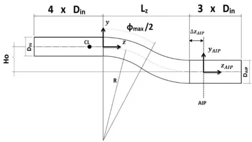
Figure 1 presents a schematic representation of the S-duct configurations simulated and the key geometrical parameters are defined. The S-ducts are characterized by a curved centreline made of two opposite circular arcs with radius R=0.665 m and angular extension Φmax/2, where Φ is the angular position along the S-duct centreline. The maximum angular extension is set to 60°, therefore Φ<30° refers to the first arc of the S-duct centreline, while Φ>30 refers to the second arc. The inlet diameter is set to 0.133m, while the offset is set to 𝐻𝑜⁄𝐷𝑖𝑛 = 1.34. The flow distortion parameters are evaluated at a cross-sectional plane, named aerodynamic interface plane (AIP), which is located at an axial distance ∆𝑧𝐴𝐼𝑃= 𝑑𝑖𝑛⁄2 downstream of the S-duct outlet. The S-ducts have a diffusing round shape with area ratio 1.52, and internal radius ri increasing along the centreline as a cubic function of the centreline position, as defined in Wellborn et al [1]. A Cartesian coordinate system is defined in Figure 1, with z-axis parallel to the centreline at the inlet, y-axis oriented along the vertical direction, and x-axis oriented perpendicular to the plane of view.
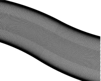
This configuration was previously experimentally investigated in [1, 8, 11, 12] and numerically analysed in MacManus et al [14, 13]. A structured mesh was created using the blocking strategy (Figure 2). The mesh used in the optimization loop has 1 million of nodes and include only half geometry. The unsteady analysis includes the whole geometry and a mesh of 6 million of nodes.
B. S-Duct Performance metrics for the optimization
The performance parameters of the S-Duct are based of the definitions of pressure recovery and swirl angle. The pressure recovery PR, the ratio between point-wise p0 and the inlet total pressure:
𝑃𝑅 =𝑝0𝑝0
𝑖𝑛 (1)
The swirl angle is defined as the ratio between the tangential and the axial components of the velocity vector [4] and represent the change of angle of attach to a compressor blade:
𝛼 = 𝑡𝑎𝑛−1(𝑢𝜃
A multi-objective optimization is conducted. Two objective functions are defined. The first quantifies the pressure losses through the S-Duct and is defined as the area-averaged pressure recovery (Equation 1) at the AIP:
𝑂𝑏𝑗𝑒𝑐𝑡𝑖𝑣𝑒 1 = 1 − 𝑃𝑅̅̅̅̅ (3) The second objective function quantifies the area-averaged swirl angle at the AIP
𝑂𝑏𝑗𝑒𝑐𝑡𝑖𝑣𝑒 2 = |𝛼|̅̅̅̅ (4) For both of the objective functions the area-average is based on the whole mesh in the AIP section. These parameters are used to quantify the S-Duct performance during the optimization process.
C. Optimization method
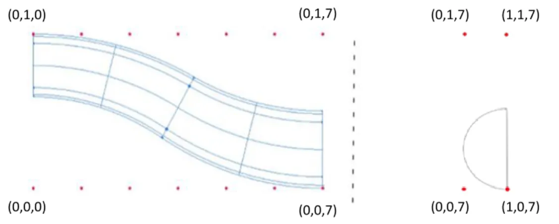
To minimize losses and swirl angle it is implemented an optimization loop which include three-dimensional free form deformation method [20] and an optimization method based on the Non-dominated Sorted Genetic Algorithm [21]. The distribution of the FFD control points is outlined in Figure 3. The Datum geometry is modified by moving the control points. The Inlet and the outlet straight duct of the domain are not modified so the control points of the FFD are located only around the S-Duct, as shown in Figure 3, and are distributed in 7 rectangular sections of four points each. The points first two and the last two sections are kept fixed to preserve the derivative at inlet and outlet section of the S-duct. The points of the symmetry plane are moving vertically, while the external points move both vertically and horizontally. The maximum movement of the control points is set to ±0.3Din.
The optimization loop was run for 5 generations. The population of each generation is set to 40 individuals. Hence, a total of 200 configurations have been simulated. For each configuration, the algorithm produces a solution vector X of 18 elements that represents the displacements of the FFD control points. The new geometry is created by means of the FFD algorithm [20], which is used also to modify the mesh blocks. A structured mesh is generated with the software ICEM through a blocking strategy. The CFD software Fluent is used to simulate the flow field of each configuration and the performance are calculated with the same methodology used in [13, 14]. For each generation the best solutions are selected to create new configurations.
D. Computational method
During the optimization loop, the objective functions of each S-Duct configurations are calculated using the results of steady-state RANS simulations. The number of iterations is set to 7000 to obtain residuals lower the 10-6 for all of the configurations. The k-ω SST configuration was selected as turbulence model for its capability to represents the flow physics of curved ducts [13] [22] [23]. In the optimization loop only half geometry is simulated to reduce the computational time because of the symmetric nature the time-averaged flow field.
In order to assess the impact of the shape optimization also on the flow fluctuations, an unsteady simulation based on Detached Eddy Simulation is conducted for the most interesting configuration. The Delayed version of the DES (DDES) [24] is used to prevent grid-induced separation problems as reported in previous versions of DES [25, 26]. In contrast with the steady-state analysis in the optimization loop, in the unsteady analysis the whole geometry is simulated. In this current work the k-ω SST turbulence model was chosen for the closure of the RANS equations. A pressure-based solver was selected with a segregated PISO scheme [27]. A second-order spatial interpolation scheme was used for the pressure equations and the third order MUSCL scheme for momentum, energy and turbulence. A bounded second order scheme [27] was used for temporal discretization with iterative time advancement with 20 sub-iterations per time step. The DDES calculations were initialized from converged RANS simulations with residuals of an order of magnitude of 10-7. Each time step was calculated using 20 sub iterations which typically resulted in residuals in the order of 10-6 for continuity equation and 10-7 for momentum, energy, k and ω equations, with a reduction of at least three orders of magnitude of all the residuals from start to end of the time step sub iterations. The time step was set to 6 μs, which corresponds to a non-dimensional time step ∆t* of 0.002. Grid sensitivity study and validation of this numerical set-up are provided in [14] for steady and unsteady simulations of S-ducts.
III.
Results
A. Results from the optimization processThe values of the objective functions of the best configurations are outlined in Figure 4. The Datum configuration is also indicated (black dot). The current Pareto front has 4 elements. The solution with minimal total pressure losses (Objective 1) is named “Opt 1” and has a reduction of 20% of the losses in comparison with the Datum configuration. The configuration with minimal swirl (Objective 2) is named “Opt 2” and has a reduction of the area-averaged swirl of 10% of the value of the Datum. Both of these optimal configurations “dominates” the Datum.
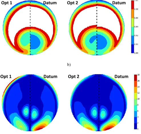
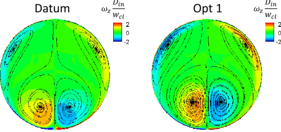
Figure 5 illustrates the AIP distribution of PR (top) and swirl angle (bottom) for the optimal configurations and the Datum. In the PR contour is evident a reduction of the losses and total pressure distortion as a shrink of the pressure deficit area. The reduction of intensity of the total pressure drop is also evident. A reduction of the swirl intensity is evident from the swirl angle distribution of both of the optimal configuration (Figure 5, b). On the other end, the secondary flow characteristics of the secondary flow at the AIP of the optimal configurations remains similar to the datum configuration, with a couple of twin-vortices on the lower part of the section (Figure 6), which is generated from the interaction between the curvature of the S-duct and the inlet boundary layer [1, 4].
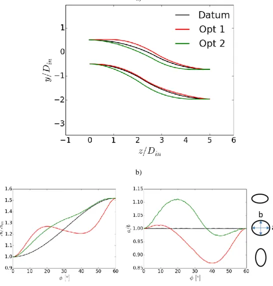
The main geometrical characteristics of the optimal configurations are illustrated in Figure 7. Comparing the shape of the symmetry plane (Figure 7a), some difference between Datum and Opt 1 configuration is observed in the first part. It is observed an upward shift of the upper-line of the Opt 1 configuration in comparison with the Datum, while the bottom lines of the two S-ducts are almost coincident. Conversely, the Opt 2 configuration is characterizes by a downward shift of the centerline in comparison with the Datum (Figure 7a). Figure 7b illustrates the distribution of the area of the cross-sections (normalized with the inlet-section area) along the centerline as a function of the angular coordinate Φ defined in Figure 1, where Φ=0° is the inlet section and Φ=60° is the outlet section of the S-duct. Remarkable difference is observed between Opt1 and the Datum configurations. The area-ratio of the Datum S-duct datum configuration has a monotonic increase towards the outlet (Figure 7b, left), which follows the cubic function defined in Wellborn et al [1]. Conversely, the Opt 1 configuration has a more abrupt increase of the area-ratio in the first part, followed by a decrease around the middle of the S-duct, and another abrupt increase close to the outlet (Φ>45°). The Opt 2 configuration has a monotonic trend of the area-ratio (Figure 7b, left) with an abrupt in increase in the first part, while the second part follow more closely the area-ratio distribution of the Datum. All of the configurations converge to A/Ain=1.52 at the outlet, since inlet and outlet sections are not modified by FFDs in the optimization process. The distribution of the “shape-factor” a/b of the sections is illustrated in Figure 7b, right, which is defined as the ratio between the width “a” and height “b”. The width “a” of is defined as the difference between the minimum and the maximum x-coordinates of the section, while the height “b” is the Euclidean distance between the highest and the lowest point of the section in the symmetry plane. The shape factor of the Datum is fixed to a/b=1.0 since its cross-section is always round. The shape of the Opt 1 configuration is ranges from 1.02 to 0.87, that is, its sections are vertically stretched, in particular in the second half of the S-duct. Conversely, the Opt 2 configuration is horizontally stretched in the first part.
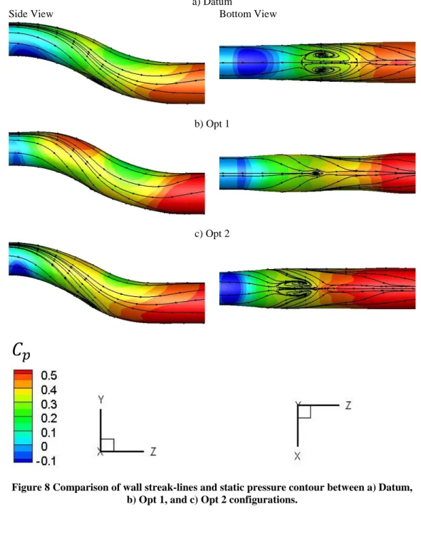
Figure 8 illustrates the streak-lines calculated from the shear stress vectors on the wall. From the side view (Figure 8, left), it is observed for all of the configurations that the boundary layer is pushed towards the bottom wall in the first part of the duct as an effect of the pressure gradient between upper and lower walls. The trace-lines from the left and right side of the duct clash of the lower part of the S-duct and generates a recirculation area with two spiral points (Figure 8, right), which represents the origin of the twin vortices observed at the AIP in Figure 6. In the second half the S-ducts the boundary layer is pushed towards the upper wall, since the direction of the pressure gradient is inverted. This effects were previously experimentally observed in Wellborn et al [1, 2]. It is noteworthy the dramatic reduction of the size of the recirculation region in the Opt 1 configuration in comparison with the Datum, which becomes almost negligible in comparison with the Datum. Previous studies suggest that a large separation bubble is the major source of instability [9] [10] [14] [13]. Therefore a reduction of the separation bubble is expected to produce a substantial reduction of the flow fluctuations. Conversely, the size of the separation bubble of the Opt 2 configuration is still comparable with the Datum configuration.
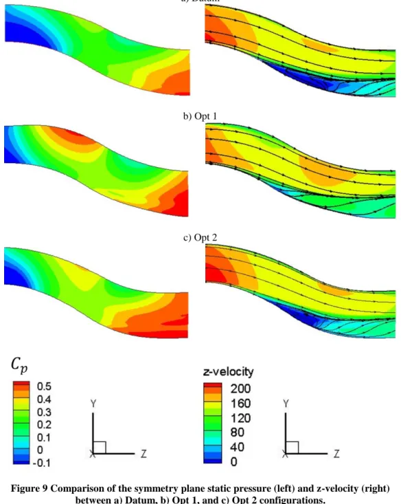
The significant shrinking of the separation bubble in the Opt 1 configuration is also evident from the axial velocity distribution and streamlines on the symmetry plane (Figure 9, right). Whilst an area of recirculation with negative velocity is evident in the Datum (blue signature in the lower side), in the Opt 1 configuration is only observed a reduction of axial velocity in the lower side of the section without any significant recirculation. A modest reduction in size of the recirculation region is observed for the Opt 2 configuration in comparison with the Datum. Overall, for all of the configurations the static pressure gradient has little effect of the mainstream flow in the symmetry plane (Figure 9), in contrast with the boundary layer flow direction observed in Figure 8. The size of the separation bubble
symmetry plane (Figure 10, left). The length of the recirculation region in calculated as the angular extension ΔΦ with negative shear stress. For the Datum the separation extends for ΔΦ=22.5°, which corresponds to a centerline length of RΔΦ≈0.261m (1.96Din), while the separation in the Opt 2 configuration extends for ΔΦ=19° with a length of approximately 0.220m (1.65Din). Hence, there is a reduction of approximately 15% of the length of the separation bubble from the Datum to the Opt 2 configuration. On the other end, the separation region in Opt extends for only 0.17Din. Moreover, the magnitude of the negative wall shear-stress coefficient of Opt 1 is much smaller in comparison with the other two configurations. In the centerline distribution of the static pressure on the lower wall it is observed that the Opt 1 configuration is also characterized by less abrupt variations of Cp along the duct in comparison with Opt 2 and Datum.
B. Unsteady simulations and dynamic distortion analysis
In this section the unsteady flow and dynamic distortion are analyzed through DDES simulations. The dominant characteristics of the flow unsteadiness are described through proper orthogonal decomposition (POD). Dynamic distortion is analyzed using the standard flow distortion descriptors defined in [5, 4, 14]. The first part is focused on the Datum configuration. This extends the previous analyses provided in [13, 14, 12]. In the second part the unsteadiness characteristics of the Datum configuration is compared with the optimal configurations Opt 1 and 2 defined in the previous section.
1. Datum configuration
The unsteady flow field of the Datum configuration is characterized by significant oscillations, which are mostly generated in the second part of the duct from the lower wall, as seen from a Q-criterion snapshot in Figure 11a. This unsteadiness produces strong fluctuations of both total pressure (Figure 11a, left) and swirl (Figure 11a, right) at the outlet section of the S-duct. It is noteworthy a signature of swirl oscillation in the middle of the lower part of the AIP with a standard deviation 20°, which is twice the mean-value of swirl observed in the average flow field in Figure 5.
Figure 12a illustrates the most dominant modes of the fluctuations of total pressure on the AIP. The modes are sorted according to their energy content. Mode 1, represents a lateral, out-of-phase oscillation of total pressure. On the other end, modes 2 and 3 combines together to reproduces a vertical oscillation of total pressure. This two modes are approximately symmetric around the symmetry plane z-y. Modes 4 adds a further orthogonal component the lateral oscillations from Mode 1. A combination of lateral and vertical oscillation of total pressure distribution was also experimentally observed in Delot et al [8] though coherence-phase analysis of unsteady total pressure measurements at the AIP. The decomposition of the velocity vector field (Figure 12b) shows that a bulk vortex with switching direction of rotation in the middle of the lower region of the AIP. This mode is associated with a continuous breaking of the symmetry of the mean field characterized by symmetric twin vortices in Figure 6. This behavior was also experimentally observed in Zachos et al [12] by means of PIV measurements. The secondary flow trace-lines and y-velocity contour in modes 2-3 clearly show a vertical oscillation of the flow field (Figure 12b). Mode 4 encompasses the bulk vortex of mode 4 with orthogonal oscillations.
To track the origin of the oscillations on the AIP, POD was also applied to the velocity field in the symmetry plane (Figure 13a). Modes 1-2 reproduces a stream-wise propagation of lateral oscillation from the lower wall in the middle of the S-duct, where the separation region in the mean flow field is located (Figure 13). From the trace-lines and the contour of x-vorticity of Modes 3-4 it is observed that the vertical oscillation at the AIP are associated with a trail of vortices propagating from the separation. The shear stress vector field on the lower wall of the duct Figure 13 show that the separation region in the mean flow (mode 0) has a behavior similar to a bluff body.
To gain more insight into the relation between the total pressure and the velocity field, a coherence analysis is conducted between the time-history lateral velocity on the lower wall of the AIP (P3 in Figure 14), where the swirl fluctuations are higher (Figure 11b) and the total pressure in two lateral points (P1 and P2 in Figure 14), where the total pressure fluctuations are higher. As expected, it is observed a peak of coherence of almost 1.0 at non-dimensional frequency St≈0.4, which is the same oscillation frequency of the POD coefficient of Mode 1 [14] (in this graph the frequency is normalized with inlet diameter and area-averaged AIP velocity). At this frequency, the x-velocity in P1 is out-of-phase with the total pressure in P2, that is, when the flow in P1 is directed to the right, the total pressure in the right region of the AIP reduces. The opposite is observed for P3. This is interpreted as a transport of low moment flow from the boundary layer in the lower wall towards the sides of the S-duct as an effect of the switching bulk vortex observed in mode 1 in Figure 12b.
2. Optimal configuration
The interesting flow field of the Opt 1 configuration is tested also with DDES-based unsteady simulations. To test the stability of the flow of the optimal configuration, the unsteady simulation of Opt 1 was initialized with highly distorted instant of the baseline configuration. Figure 15 compares the time history of the total pressure (top) and swirl (bottom) coefficients defined in [14] of the Datum and the Opt 1 configurations. It is evident the high reduction of the fluctuations in the optimal configuration with remarkable reduction of peak values of distortion and time-averaged values, in particular for swirl. The distribution of the DDES blending function fd [28] in Figure 16 (left) show that the LES part of the simulation is correctly activated after the separation in both the Datum and the Opt 1 configuration. The increase of fd towards 1.0 produces a dramatic reduction of the of the turbulent viscosity which allowed the development of significant oscillation in the flow field of the Datum configuration. However, very small oscillations are observed in the Opt 1 configuration, which suggests a much more stable flow field as a result of the highly reduced size of the recirculation region (Figure 8 and Figure 9) and a less abrupt variation of static pressure along the centerline (Figure 10).
The improvement of the performance is also observed from the distortion maps in Figure 17. The red dot in the maps indicate the distortion calculated from the time-averaged mean field (static distortion). The distortion parameters in Figure 17 are defined in [5] [4] [14], and are calculated from a conventional equal-area 8x5 rake defined in [5, 14]. The datum is characterized by strong oscillation of the distortion metrics, with circumferential distortion oscillating from 0.01 to 0.05, with a peak value 2.5 times higher the static distortion (red dot). Even more dramatic is the oscillation of the swirl parameters SD-SI in the Datum. The mean flow (red dot) has a swirl directivity SD=0.0, which means that the secondary flow is substantially symmetric (see Figure 6). However, the map of Figure 17a (left) shows that unsteady flow field oscillates from SD=1.0 to -1.0, that is, the twin vortices in the mean field (Figure 6) are periodically switched to a bulk vortex with alternate rotation of direction. This switch is associated with a dramatic increase of the swirl intensity SI [4], which represents the area-averaged swirl over an 8x5 rake [14], with peak values approximately five times the static value. It is of note that the swirl directivity of Opt 1 (Figure 17b) remains zero instead of oscillating between -1 and 1, which suggests that the lateral oscillation of the Datum configuration described in [14] [11] [12], associated with an increase of distortion, are absent in the Opt 1 configuration. An increased stability of the flow is important because it was previously observed that a compressor surge can be trigger also by instantaneous peaks of distortion [15].
The reduction of the dynamic distortion in the Opt 2 is less remarkable (Figure 17c). However, the POD analysis of the flow oscillations (Figure 18) provides interesting information. It is observed that the AIP flow field fluctuations of the Opt 2 configuration are mostly dominated by vertical oscillations (Mode 1-2 in Figure 18), in contrast with the Datum configuration which is dominated by lateral oscillations a vorticity (Mode 1 in Figure 12). The lateral oscillation is located in Mode 3 for the Opt 2 configuration, that is, it is less dominant. Another interesting characteristics is observed from the spectral distribution of the POD coefficient the Modes 1-4. Indeed, in Figure 18c, left, the lateral oscillation mode of the Opt 2 configuration is shifted-up in frequency of about 15% in comparison with the lateral model of the Datum (Figure 18c, left). Indeed, the Strouhal number Std in the left of Figure 18c is simply based of the inlet diameter Din and the inlet axial velocity wcl, which are identical for both of the configurations. It is surmised that this increased in frequency from Datum to Opt 2 is related to the reduction 15% of the length of the separation region quantified in section III.A. Indeed, replacing the inlet diameter with the length of the separation region in each configuration in the Strouhal number definition, the non-dimensional frequencies of the lateral oscillation become approximately coincident (Figure 18c, right). A more remarkable shift in frequency is observed for the vertical modes, where the frequency of the vertical Modes 1-2 in the Opt 2 configuration is approximately 50% higher than the corresponding vertical modes 2-3 of the Datum.
IV.
Conclusion
In this work it is conducted a shape optimization of an S-Duct by means of free form deformation coupled with a genetic algorithm. Currently the optimization has produced a Pareto front of 4 points. One extreme point of the front has a reduction of the total pressure losses of the 20% while the other has a reduction of the area-averaged swirl of 10%. Further reduction is expected increasing the range of variation of the control points.
The unsteadiness of the flow field was also tested by means of Delayed-Detached Eddy Simulations. Surprisingly the configuration with minimal losses was characterized by a very stable flow with a huge reduction of the flow fluctuations which produces a strong reduction of the flow distortion.
References
[1] S. R. Wellborn, T. H. Okiishi and B. A. Reichert, "A study of the Compressible Flow Through a Diffusing S-Duct," NASA Technical Memorandum 106411, 1993.
[2] S. R. Wellborn, B. A. Reichert and T. H. Okiishi, "An Experimental Investigation of the Flow in a Diffusing S-Duct," in 28th Joint Propulsion Conference and Exhibit, Nashville, Tennessee, July 6-8, AIAA Paper 1992-3622, 1992.
[3] G. J. Harloff, B. A. Reichert and S. R. Wellborn, "Navier-Stokes Analysis and Experimental Data Comparison of Compressible Flow in a Diffusing S-Duct," in 10th Applied Aerodynamics Conference, Fluid Dynamics and Co-located Conferences, AIAA Paper 92-2699, 1992.
[4] S-16 Turbine Engine Inlet Flow Distortion Committe, "A Methodology for Assessing Inlet Swirl Distortion," No. AIR1419, Society of Automotive Engineers, 2007.
[5] Society of Automotive Engineering, Inlet Total-Pressure-Distortion Considerations for Gas-Turbine Engines, Warrendale, PA, 1999.
[6] W. Meyer, W. Pazur and L. Fottner, "The Influence of Intake Swirl Distortion on the Steady-State Performance of a Low Bypass Twin-Spool Engine," Tech. Rep. CP-498, AGARD, 1991.
[7] G. A. Mitchell, "Effect of Inlet Ingestion of a Wing Tip Vortex on Compressor Face Flow and Turbojet Stall Margin," Tech. Rep. TM X-3246, NASA, 1975.
[8] A.-L. Delot, E. Garnier and D. Pagan, "Flow Control in a High-Offset Subsonic Air Intake," in 47th AIAA/ASME/SAE/ASEE Joint Propuslion Conference & Exibit, San Diego, California, USA, AIAA Paper 2011-5569, 2011.
[9] E. Garnier, "Flow Control by Pulsed Jet in a Curved S-Duct:," AIAA JOURNAL, vol. 53, no. 10, October 2015. [10] E. Garnier, M. Leplat, J. C. Monnier and J. Delva, "Flow control by pulsed jet in a highly bended S-duct," in
6th AIAA Flow Control Conference 25 - 28 June 2012, New Orleans, Louisiana, AIAA Paper 2012-3250, 2012. [11] P. Zachos, D. G. MacManus and N. Chiereghin, "Flow distortion measurements in convoluted aero engine
intakes," in 33rd AIAA Applied Aerodynamics Conference, AIAA Aviation, Dallas, AIAA Paper 2015-3305, 2014.
[12] P. Zachos, D. G. MacManus, D. Gil Prieto and N. Chiereghin, "Flow Distortion Measurements in Convoluted Aeroengine Intakes," AIAA Journal, Vols. 54, Special Section on Evaluation of RANS Solvers on Benchmark Aerodynamics Flows, 2016, pp 2819-2832.
[13] N. Chiereghin, D. G. MacManus, M. Savill and R. Dupuis, "Dynamic distortion simulations for curved aeronautical intakes," in Advanced Aero-concepts, Design and Operations, Royal Aeronautical Society Applied Aerodynamics Conference, Bristol, 2014.
[14] D. G. MacManus, N. Chiereghin, D. Gil Prieto and P. Zachos, "Complex aero-engine intake ducts and dynamic distortion," in AIAA Aviation and Aeronautics Forum and Exposition, Dallas, USA, AIAA Paper 2015-3304, 2015.
[15] D. N. Bowditch and R. E. Coltrin, "A Survey of Inlet/Engine Distortion Compatibility," NASA Technical Memorandum TM-83421, 1983.
[16] B. J. Wendt and B. A. Reichert, "Vortex ingestion in a diffusing S-duct inlet," Journal of Aircraft, vol. 33, no. 1, pp. 149-154, 1996.
[17] W. Zhang, D. D. Knight and D. Smith, "Automated Design of a Three-Dimensional Subsonic Diffuser",,," Journal of Propulsion and Power, vol. 16, no. 6, pp. 1132-1140, 2000.
[18] A. Aranake, J. G. Lee, D. D. Knight, R. M. Cummings, J. Cox, M. Paul and A. R. Byerley, "Automated Design Optimization of a Three-Dimensional Subsonic Diffuser," Journal of Propulsion AND Power, vol. 27, no. 4, pp. 838-846, 2011.
[19] F. Furlan, N. Chiereghin, T. Kipouros, E. Benini and M. Savill, "Computational design of S-Duct intakes for distributed propulsion",," Aircraft Engineering and Aerospace Technology: An International Journal, vol. 86, no. 6, pp. 473 - 477, 2014.
[20] T. W. Sederberg and S. R. Parry, "Free-form deformation of solid geometric models," ACM SIGGRAPH Computer Graphics, vol. 20, no. 4, pp. 151-160, 1986.
[21] K. Deb, Multi-Objective Optimization using Evolutionary Algorithms, Wiley, 2001.
[22] A.-L. Delot and R. K. Schamhorst, "A Comparison of Several CFD Codes with Experimental Data in a Diffusing S-Duct," in 49th AIAA/ASME/SAE/ASEE Joint Propulsion Conference, San Jose, USA, AIAA Paper 2013-3796, 2013.
[23] C. Fiola and R. K. Agarwal, "Simulation of Secondary and Separated Flow in Diffusing S Ducts," Journal of Propulsion and Power, vol. 31, no. 1, pp. 180-191, 2015.
[24] P. R. Spalart, S. Deck, M. L. Shur, K. D. Squires, M. K. Strelets and A. Travin, "A New Version of Detached-eddy Simulation, Resistant to Ambiguous Grid Densities," Theoretical and Computational Fluid Dynamics, vol. 20, no. 3, pp. 181-195, 2006.
[25] M. Chevalier and S. H. Peng, "Detached Eddy Simulation of Turbulent Flow in a Highly Offset Intake Diffuser," in Progress in Hybrid RANS-LES Modelling, Verlag Berlin Heidelberg , Springer, 2010, pp. 111-121.
[26] P. S. Spalart, "Detached-Eddy Simulation," The Annual Review of Fluid Mechanics, vol. 41, pp. 181-202, 2008. [27] ANSYS, ANSYS FLUENT User Guide, Southpointe, 275 Technology Drive, Canonsburg, PA, 15317, 2011. [28] M. S. Gritskevich, A. V. Garbaruk, J. Schütze and F. R. Menter, "Development of DDES and IDDES
Formulations for the k-ω Shear Stress Transport Model," Flow, Turbulence and Combustion, vol. 88, no. 3, 2014, pp. 431-449.
a)
b)
Figure 2 Structured mesh for the Datum S-Duct: a) side view, b) front view at the outlet of the S-Duct.
a) b)
Figure 3 Control points distribution around the Datum configuration: a) side view, b) front view at the outlet of the S-Duct.
Y (0,0,0) (0,0,7) (0,1,7) (0,1,0) (0,0,7) (1,0,7) (0,1,7) (1,1,7)
Figure 4 Objective functions of the best configurations and Pareto front compared with the Datum configuration (black dot).
Opt 1
Opt 2
Objective 1 Objective 2
a)
b)
Figure 5 Comparison between Datum and optimal S-Ducts at the AIP: a) pressure recovery, b) swirl angle (degrees).
Opt 1
Datum
Opt 2
Datum
Figure 6 AIP distribution of z-vorticity ωz (out-of-plane) with trace-lines of the secondary
flow; comparison between Datum (left) and Opt 1 (right) configurations.
a)
b)
Figure 7 Main geometrical characteristics of the datum (black), Opt 1 (red) and Opt 2 (green) configurations: a) symmetry plane, b) centerline distribution of area-ratio (left) and shape-factor
(right).
a
b
a) Datum
Side View Bottom View
b) Opt 1
c) Opt 2
Figure 8 Comparison of wall streak-lines and static pressure contour between a) Datum, b) Opt 1, and c) Opt 2 configurations.
a) Datum
b) Opt 1
c) Opt 2
Figure 9 Comparison of the symmetry plane static pressure (left) and z-velocity (right) between a) Datum, b) Opt 1, and c) Opt 2 configurations.
Figure 10 Centerline distribution of A) z-component of the skin friction coefficient Cf,z on
a)
b)
Figure 11 Flow field unsteadiness of the Datum configuration: a) Three-dimensional Q-criterion iso-surfaces from a snapshot of the DDES simulation, b) AIP distribution of the standard deviation of pressure recovery (left) and swirl angle (right). Adapted from MacManus
a) PR
Mode 1 Mode 2 Mode 3 Mode 4
b) u,v,w
Mode 1 Mode 2 Mode 3 Mode 4
Figure 12 POD modes on the AIP from DDES of the Datum configuration.
a) Symmetry plane
b) Wall, bottom View
Figure 13 POD modes from DDES simulation of the Datum configuration: a) velocity vector field on the symmetry plane, b) wall shear-stress vector.
Mode 1
Mode 2
Mode 4
Mode 3
Mode 0 Mode 1
Figure 14 Coherence and phase on the AIP between time-history of lateral velocity at the point P3 and total pressure at the points P1 (top) and P2 (bottom).
u P3
P2 P1
Figure 15 Comparison of time-history of total pressure distortion coefficient (top) and swirl coefficient (bottom) between Datum (left) and Opt 1 configurations (right).
baseline
optimal
transition
a) Datum
b) Opt 1
Figure 16 Symmetry plane distribution of the DDES blending function fd [28] (left) and
turbulent viscosity (right).
DDES Blending function, fd Turbulent viscosity
a) Datum
b) Opt 1
c) Opt 2
Figure 17 Maps of instantaneous flow distortion at the AIP: a) radial against circumferential total pressure distortion, b) swirl directivity against swirl intensity.
a) modes PR
Mode 1 Mode 2 Mode 3 Mode 4
b) modes u,v,w
Mode 1 Mode 2 Mode 3 Mode 4
c) Fourier transform PR
Figure 18 POD modes on the Opt 2 configuration.