7 Two-dimensional NMR

7

Two-dimensional NMR

†

7.1 Introduction

The basic ideas of two-dimensional NMR will be introduced by reference to the appearance of a COSY spectrum; later in this chapter the product operator formalism will be used to predict the form of the spectrum.

Conventional NMR spectra (one-dimensional spectra) are plots of intensity

vs. frequency; in two-dimensional spectroscopy intensity is plotted as a function of two frequencies, usually called F₁ and F₂. There are various ways of representing such a spectrum on paper, but the one most usually used is to make a contour plot in which the intensity of the peaks is represented by contour lines drawn at suitable intervals, in the same way as a topographical map. The position of each peak is specified by two frequency co-ordinates corresponding to F₁ and F₂. Two-dimensional NMR spectra are always arranged so that the F₂

co-ordinates of the peaks correspond to those found in the normal dimensional spectrum, and this relation is often emphasized by plotting the one-dimensional spectrum alongside the F₂ axis.

The figure shows a schematic COSY spectrum of a hypothetical molecule containing just two protons, A and X, which are coupled together. The one-dimensional spectrum is plotted alongside the F₂ axis, and consists of the familiar pair of doublets centred on the chemical shifts of A and X, δ_A and δ_X respectively. In the COSY spectrum, the F₁ co-ordinates of the peaks in the two-dimensional spectrum also correspond to those found in the normal one-dimensional spectrum and to emphasize this point the one-one-dimensional spectrum has been plotted alongside the F₁ axis. It is immediately clear that this COSY spectrum has some symmetry about the diagonal F₁ = F₂ which has been indicated with a dashed line.

In a one-dimensional spectrum scalar couplings give rise to multiplets in the spectrum. In two-dimensional spectra the idea of a multiplet has to be expanded somewhat so that in such spectra a multiplet consists of an array of individual peaks often giving the impression of a square or rectangular outline. Several such arrays of peaks can be seen in the schematic COSY spectrum shown above. These two-dimensional multiplets come in two distinct types:

diagonal-peak multiplets which are centred around the same F₁ and F₂

frequency co-ordinates and cross-peak multiplets which are centred around different F₁ and F₂ co-ordinates. Thus in the schematic COSY spectrum there are two diagonal-peak multiplets centred at F₁ = F₂ = δ_A and F₁ = F₂ = δ_X, one cross-peak multiplet centred at F₁ = δ_A, F₂ = δ_X and a second cross-peak multiplet centred at F₁= δ_X, F₂= δ_A.

The appearance in a COSY spectrum of a cross-peak multiplet F₁ = δ_A, F₂=

δX indicates that the two protons at shifts δA and δX have a scalar coupling

†

Chapter 7 "Two-Dimensional NMR" © James Keeler 1998 and 2002

δ_A

δX

δ_A δX

Schematic COSY spectrum for two coupled spins, A and X

between them. This statement is all that is required for the analysis of a COSY spectrum, and it is this simplicity which is the key to the great utility of such spectra. From a single COSY spectrum it is possible to trace out the whole coupling network in the molecule

7.1.1 General Scheme for two-Dimensional NMR

In one-dimensional pulsed Fourier transform NMR the signal is recorded as a function of one time variable and then Fourier transformed to give a spectrum which is a function of one frequency variable. In two-dimensional NMR the signal is recorded as a function of two time variables, t₁ and t₂, and the resulting data Fourier transformed twice to yield a spectrum which is a function of two frequency variables. The general scheme for two-dimensional spectroscopy is

evolution detection

t₁ mixing t₂

preparation

In the first period, called the preparation time, the sample is excited by one or more pulses. The resulting magnetization is allowed to evolve for the first time period, t₁. Then another period follows, called the mixing time, which consists of a further pulse or pulses. After the mixing period the signal is recorded as a function of the second time variable, t₂. This sequence of events is called a pulse sequence and the exact nature of the preparation and mixing periods determines the information found in the spectrum.

It is important to realize that the signal is not recorded during the time t₁, but only during the time t₂ at the end of the sequence. The data is recorded at regularly spaced intervals in both t₁and t₂.

The two-dimensional signal is recorded in the following way. First, t₁ is set to zero, the pulse sequence is executed and the resulting free induction decay recorded. Then the nuclear spins are allowed to return to equilibrium. t₁ is then set to ∆₁, the sampling interval in t₁, the sequence is repeated and a free induction decay is recorded and stored separately from the first. Again the spins are allowed to equilibrate, t₁ is set to 2∆₁, the pulse sequence repeated and a free induction decay recorded and stored. The whole process is repeated again for t₁= 3∆₁, 4∆₁ and so on until sufficient data is recorded, typically 50 to 500 increments of t₁. Thus recording a two-dimensional data set involves repeating a pulse sequence for increasing values of t₁ and recording a free induction decay as a function of t₂ for each value of t₁.

7.1.2 Interpretation of peaks in a two-dimensional spectrum

Within the general framework outlined in the previous section it is now possible to interpret the appearance of a peak in a two-dimensional spectrum at particular frequency co-ordinates.

F₁

F₂

0,0 80

20

a b c

Suppose that in some unspecified two-dimensional spectrum a peak appears at

F₁ = 20 Hz, F₂ = 80 Hz (spectrum a above) The interpretation of this peak is that a signal was present during t₁ which evolved with a frequency of 20 Hz. During the mixing time this same signal was transferred in some way to another signal which evolved at 80 Hz during t₂.

Likewise, if there is a peak at F₁ = 20 Hz, F₂ = 20 Hz (spectrum b) the interpretation is that there was a signal evolving at 20 Hz during t₁ which was unaffected by the mixing period and continued to evolve at 20 Hz during t₂. The processes by which these signals are transferred will be discussed in the following sections.

Finally, consider the spectrum shown in c. Here there are two peaks, one at

F₁ = 20 Hz, F₂ = 80 Hz and one at F₁ = 20 Hz, F₂ = 20 Hz. The interpretation of this is that some signal was present during t₁ which evolved at 20 Hz and that during the mixing period part of it was transferred into another signal which evolved at 80 Hz during t₂. The other part remained unaffected and continued to evolve at 20 Hz. On the basis of the previous discussion of COSY spectra, the part that changes frequency during the mixing time is recognized as leading to a cross-peak and the part that does not change frequency leads to a diagonal-peak. This kind of interpretation is a very useful way of thinking about the origin of peaks in a two-dimensional spectrum.

It is clear from the discussion in this section that the mixing time plays a crucial role in forming the two-dimensional spectrum. In the absence of a mixing time, the frequencies that evolve during t₁ and t₂ would be the same and only diagonal-peaks would appear in the spectrum. To obtain an interesting and useful spectrum it is essential to arrange for some process during the mixing time to transfer signals from one spin to another.

7.2 EXSY and NOESY spectra in detail

In this section the way in which the EXSY (EXchange SpectroscopY) sequence works will be examined; the pulse sequence is shown opposite. This experiment gives a spectrum in which a cross-peak at frequency co-ordinates F₁

= δ_A, F₂ = δ_B indicates that the spin resonating at δ_A is chemically exchanging with the spin resonating at δ_B.

The pulse sequence for EXSY is shown opposite. The effect of the sequence will be analysed for the case of two spins, 1 and 2, but without any coupling between them. The initial state, before the first pulse, is equilibrium

t₁ τ t2

mix

The pulse sequence for EXSY (and NOESY). All pulses have 90° flip angles.

magnetization, represented as I_1z + I_2z; however, for simplicity only magnetization from the first spin will be considered in the calculation.

The first 90° pulse (of phase x) rotates the magnetization onto –y

I_z Ix Ix I_y 1 2 2 1 1 2 π π  →  −→

(the second arrow has no effect as it involves operators of spin 2). Next follows evolution for time t₁

−I _y t Iz→  −t Iz→ t I_y + t I_x

1 1 1 1 1 1 1

1 1 1 2 1 2

Ω Ω _{cosΩ sinΩ}

again, the second arrow has no effect. The second 90° pulse turns the first term onto the z-axis and leaves the second term unaffected

−  →  −→  → → cos cos sin sin Ω Ω Ω Ω 1 1 1 2 2 1 1 1 1 1 1 2 2 1 1 1 1 2 1 2 t I t I t I t I y I I z x I I x x x x x π π π π

Only the I_1z term leads to cross-peaks by chemical exchange, so the other term will be ignored (in an experiment this is achieved by appropriate coherence pathway selection). The effect of the first part of the sequence is to generate, at the start of the mixing time, τ_mix, some z-magnetization on spin 1 whose size depends, via the cosine term, on t₁ and the frequency, Ω₁, with which the spin 1 evolves during t₁. The magnetization is said to be frequency labelled.

During the mixing time, τ_mix, spin 1 may undergo chemical exchange with spin 2. If it does this, it carries with it the frequency label that it acquired during t₁. The extent to which this transfer takes place depends on the details of the chemical kinetics; it will be assumed simply that during τ_mix a fraction f of the spins of type 1 chemically exchange with spins of type 2. The effect of the mixing process can then be written

−cosΩ_{1 1}t I_1z mixing − −→

(

1 f

)

cosΩ_{1 1}t I_1z − f cosΩ_{1 1}t I_2z

The final 90° pulse rotates this z-magnetization back onto the y-axis

− −

(

)

 → →

(

−

)

−  → → 1 _{1 1 1} 2 2 1 _{1 1 1} 1 1 2 2 2 1 1 2 1 2 1 2 f t I f t I f t I f t I z I I y z I I y x x x x cos cos cos cos Ω Ω Ω Ω π π π π

Although the magnetization started on spin 1, at the end of the sequence there is magnetization present on spin 2 – a process called magnetization transfer. The analysis of the experiment is completed by allowing the I_1y and I_2y

operators to evolve for time t₂. 1 1 1 1 1 1 1 2 1 1 1 1 2 1 1 1 1 1 2 2 2 1 1 2 1 2 1 2 2 2 1 2 1 2 2 2 −

(

)

 → → −

(

)

− −

(

)

 → → f t I f t t I f t t I f t I f t t I y t I t I y x y t I t I z z z z cos

cos cos sin cos

cos cos cos Ω Ω Ω Ω Ω Ω Ω Ω Ω Ω Ω Ω yy − fsinΩ2 2t cosΩ1 1t I2x

If it is assumed that the y-magnetization is detected during t₂ (this is an arbitrary choice, but a convenient one), the time domain signal has two terms:

1− _{1 2 1 1 2 2 1 1}

(

f

)

cosΩt cosΩt + f cosΩ t cosΩt

The crucial thing is that the amplitude of the signal recorded during t₂ is modulated by the evolution during t₁. This can be seen more clearly by imagining the Fourier transform, with respect to t₂, of the above function. The cosΩ_{1 2}t and cosΩ_{2 2}t terms transform to give absorption mode signals centred at Ω₁ and Ω₂ respectively in the F₂ dimension; these are denoted A₁( )2 and A₂( )2

(the subscript indicates which spin, and the superscript which dimension). The time domain function becomes

1− ₁2 _{1 1 2}2 _{1 1}

(

f A

)

( )cosΩt + fA( )cosΩt

If a series of spectra recorded as t₁ progressively increases are inspected it would be found that the cosΩ_{1 2}t term causes a change in size of the peaks at Ω₁ and Ω₂ – this is the modulation referred to above.

Fourier transformation with respect to t₁ gives peaks with an absorption lineshape, but this time in the F₁ dimension; an absorption mode signal at Ω₁ in

F₁ is denoted A₁( )1. The time domain signal becomes, after Fourier transformation in each dimension

1− ₁2 ₁1 ₂2 ₁1

(

f A A

)

( ) ( )+ fA A( ) ( )

Thus, the final two-dimensional spectrum is predicted to have two peaks. One is at (F₁, F₂) = (Ω₁, Ω₁) – this is a diagonal peak and arises from those spins of type 1 which did not undergo chemical exchange during τ_mix. The second is at (F₁, F₂) = (Ω₁, Ω₂) – this is a cross peak which indicates that part of the magnetization from spin 1 was transferred to spin 2 during the mixing time. It is this peak that contains the useful information. If the calculation were repeated starting with magnetization on spin 2 it would be found that there are similar peaks at (Ω₂, Ω₂) and (Ω₂, Ω₁).

The NOESY (Nuclear Overhauser Effect SpectrocopY) spectrum is recorded using the same basic sequence. The only difference is that during the mixing time the cross-relaxation is responsible for the exchange of magnetization between different spins. Thus, a cross-peak indicates that two spins are experiencing mutual cross-relaxation and hence are close in space.

Having completed the analysis it can now be seen how the EXCSY/NOESY sequence is put together. First, the 90° – t₁ – 90° sequence is used to generate frequency labelled z-magnetization. Then, during τ_mix, this magnetization is allowed to migrate to other spins, carrying its label with it. Finally, the last pulse renders the z-magnetization observable.

7.3 More about two-dimensional transforms

From the above analysis it was seen that the signal observed during t₂ has an amplitude proportional to cos(Ω₁t₁); the amplitude of the signal observed during

t₂ depends on the evolution during t₁. For the first increment of t₁ (t₁ = 0), the signal will be a maximum, the second increment will have size proportional to cos(Ω₁∆₁), the third proportional to cos(Ω₁2∆₁), the fourth to cos(Ω₁3∆₁) and so

time

frequency

Ω

Fourier transform

The Fourier transform of a decaying cosine function cosΩt e x p ( –t/T2) i s a n

absorption mode Lorentzian centred at frequency Ω; the real part of the spectrum has been plotted.

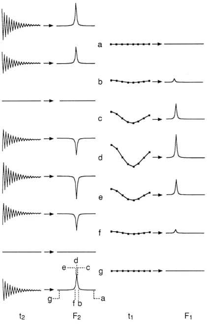
on. This modulation of the amplitude of the observed signal by the t₁ evolution is illustrated in the figure below.

In the figure the first column shows a series of free induction decays that would be recorded for increasing values of t₁ and the second column shows the Fourier transforms of these signals. The final step in constructing the two-dimensional spectrum is to Fourier transform the data along the t₁ dimension. This process is also illustrated in the figure. Each of the spectra shown in the second column are represented as a series of data points, where each point corresponds to a different F₂ frequency. The data point corresponding to a particular F₂ frequency is selected from the spectra for t₁ = 0, t₁ = ∆₁, t₁ = 2∆₁ and so on for all the t₁ values. Such a process results in a function, called an

interferogram, which has t₁ as the running variable.

two-dimensional spectrum. In the left most column is shown a series of free induction decays that would be recorded for successive values of t1; t1 increases down the page. Note how the amplitude of these free

induction decays varies with t₁, something that becomes even plainer when the time domain signals are Fourier transformed, as shown in the second column. In practice, each of these F2 spectra in column two

consist of a series of data points. The data point at the same frequency in each of these spectra is extracted and assembled into an interferogram, in which the horizontal axis is the time t1. Several such

interferograms, labelled a to g, are shown in the third column. Note that as there were eight F₂ spectra in column two corresponding to different t1 values there are eight points in each interferogram. The F2

frequencies at which the interferograms are taken are indicated on the lower spectrum of the second column. Finally, a second Fourier transformation of these interferograms gives a series of F1 spectra shown

in the right hand column. Note that in this column F₂ increases down the page, whereas in the first column t₁

increase down the page. The final result is a two-dimensional spectrum containing a single peak.

Several interferograms, labelled a to g, computed for different F₂ frequencies are shown in the third column of the figure. The particular F₂ frequency that each interferogram corresponds to is indicated in the bottom spectrum of the second column. The amplitude of the signal in each interferogram is different, but in this case the modulation frequency is the same. The final stage in the processing is to Fourier transform these interferograms to give the series of spectra which are shown in the right most column of the figure. These spectra have F₁ running horizontally and F₂ running down the page. The modulation of the time domain signal has been transformed into a single two-dimensional peak. Note that the peak appears on several traces corresponding to different F₂

frequencies because of the width of the line in F₂.

The time domain data in the t₁ dimension can be manipulated by multiplying by weighting functions or zero filling, just as with conventional free induction decays.

7.4 Two-dimensional experiments using coherence transfer

through J-coupling

Perhaps the most important set of two-dimensional experiments are those which transfer magnetization from one spin to another via the scalar coupling between them. As was seen in section 6.3.3, this kind of transfer can be brought about by the action of a pulse on an anti-phase state. In outline the basic process is

Ix I Iy z I I

x

z y

1 2 1 2 2 1 2

coupling 90 ( ) to both spins

spin 1 spin 2

→ ° →

7.4.1 COSY

The pulse sequence for this experiment is shown opposite. It will be assumed in the analysis that all of the pulses are applied about the x-axis and for simplicity the calculation will start with equilibrium magnetization only on spin 1. The effect of the first pulse is to generate y-magnetization, as has been worked out previously many times

I_z Ix Ix I _y 1 2 2 1 1 2 π π  →  −→

This state then evolves for time t₁, first under the influence of the offset of spin 1 (that of spin 2 has no effect on spin 1 operators):

−I_y  −t Iz→ t I _y+ t I _x

1 1 1 1 1 1 1

1 1 1

Ω _{cosΩ sinΩ}

t₁ t2

Pulse sequence for the two-dimensional COSY experiment

Both terms on the right then evolve under the coupling

−  −→ +

→ +

cos cos cos sin cos

sin cos sin sin sin

Ω Ω Ω Ω Ω Ω 1 1 1 2 12 1 1 1 1 12 1 1 1 1 2 1 1 1 2 12 1 1 1 1 12 1 1 1 1 12 1 1 2 12 1 1 2 2 2 t I J t t I J t t I I t I J t t I J t t I I y J t I I y x z x J t I I x y z z z z π π π π π π 22z

That completes the evolution under t₁. Now all that remains is to consider the effect of the final pulse, remembering that the effect of the pulse on both spins needs to be computed. Taking the terms one by one:

−  →  −→

{ }

 →  −→

_{{ }}

cos cos cos cos

sin cos sin cos

cos sin π π π π π π π π π J t t I J t t I J t t I I J t t I I J t y I I z x z I I x y x x x x 12 1 1 1 1 2 2 12 1 1 1 1 12 1 1 1 1 2 2 2 12 1 1 1 1 2 12 1 1 2 1 2 1 2 2 2 Ω Ω Ω Ω Ω Ω Ω Ω Ω 1 1 1 2 2 12 1 1 1 1 12 1 1 1 1 2 2 2 12 1 1 1 1 2 1 2 1 2 3 2 2 4 t I J t t I J t t I I J t t I I x I I x y z I I z y x x x x π π π π π π π  → →

{ }

 →  −→

_{{ }}

cos sin

sin sin sin sin

Terms {1} and {2} are unobservable. Term {3} corresponds to in-phase magnetization of spin 1, aligned along the x-axis. The t₁ modulation of this term depends on the offset of spin 1, so a diagonal peak centred at (Ω₁,Ω₁) is predicted. Term {4} is the really interesting one. It shows that anti-phase magnetization on spin 1, 2I I_{1y 2z}, is transferred to anti-phase magnetization on spin 2, 2I I_{1z 2y}; this is an example of coherence transfer. Term {4} appears as observable magnetization on spin 2, but it is modulated in t₁ with the offset of spin 1, thus it gives rise to a cross-peak centred at (Ω₁,Ω₂). It has been shown, therefore, how cross- and diagonal-peaks arise in a COSY spectrum.

Some more consideration should be give to the form of the cross- and diagonal peaks. Consider again term {3}: it will give rise to an in-phase multiplet in F₂, and as it is along the x-axis, the lineshape will be dispersive. The form of the modulation in t₁ can be expanded, using the formula,

cos sinA B= 1

{

sin

(

B+A

)

+sin

(

B−A

)

}

2 to give

cosπJ t_{12 1}sin _{1 1}t 1 sin t πJ t sin t πJ t

2 1 1 12 1 1 1 12

Ω =

{

(

Ω +

)

+

(

Ω −

)

}

Two peaks in F₁ are expected at Ω₁±πJ₁₂, these are just the two lines of the spin 1 doublet. In addition, since these are sine modulated they will have the dispersion lineshape. Note that both components in the spin 1 multiplet observed in F₂ are modulated in this way, so the appearance of the two-dimensional multiplet can best be found by "multiplying together" the multiplets in the two dimensions, as shown opposite. In addition, all four components of the diagonal-peak multiplet have the same sign, and have the double dispersion lineshape illustrated below

time

frequency

Ω

Fourier transform

The Fourier transform of a d e c a y i n g s i n e f u n c t i o n sinΩt exp(–t/T2) is a dispersion

mode Lorentzian centred at frequency Ω.

F₁ J₁₂

F₂ J₁₂

Schematic view of the diagonal peak from a COSY spectrum. The squares are supposed to indicate the two-dimensional double dispersion lineshape illustrated below

The double dispersion lineshape seen in pseudo 3D and as a contour plot; negative contours are indicated by dashed lines.

Term {4} can be treated in the same way. In F₂ we know that this term gives rise to an anti-phase absorption multiplet on spin 2. Using the relationship

sinBsinA= 1

{

−cos

(

B+A

)

+cos

(

B−A

)

}

2 the modulation in t1 can be expanded

sinπJ t_{12 1}sin ₁t 1 cos t πJ t cos t πJ t

2 1 1 12 1 1 1 12

Ω =

{

−

(

Ω +

)

+

(

Ω −

)

}

Two peaks in F₁, at Ω₁±πJ₁₂, are expected; these are just the two lines of the spin 1 doublet. Note that the two peaks have opposite signs – that is they are anti-phase in F₁. In addition, since these are cosine modulated we expect the absorption lineshape (see section 7.2). The form of the cross-peak multiplet can be predicted by "multiplying together" the F₁ and F₂ multiplets, just as was done for the diagonal-peak multiplet. The result is shown opposite. This characteristic pattern of positive and negative peaks that constitutes the cross-peak is know as an anti-phase square array.

The double absorption lineshape seen in pseudo 3D and as a contour plot.

COSY spectra are sometimes plotted in the absolute value mode, where all the sign information is suppressed deliberately. Although such a display is convenient, especially for routine applications, it is generally much more desirable to retain the sign information. Spectra displayed in this way are said to be phase sensitive; more details of this are given in section 7.6.

As the coupling constant becomes comparable with the linewidth, the positive and negative peaks in the cross-peak multiplet begin to overlap and cancel one another out. This leads to an overall reduction in the intensity of the cross-peak multiplet, and ultimately the cross-peak disappears into the noise in the spectrum. The smallest coupling which gives rise to a cross-peak is thus set

F₁ J₁₂

F₂ J₁₂

Schematic view of the cross-peak multiplet from a COSY spectrum. The circles are supposed to indicate the two-dimensional double absorption lineshape illustrated below; filled circles represent positive intensity, open represent negative intensity.

by the linewidth and the signal-to-noise ratio of the spectrum.

7.4.2 Double-quantum filtered COSY (DQF COSY)

The conventional COSY experiment suffers from a disadvantage which arises from the different phase properties of the cross- and diagonal-peak multiplets. The components of a diagonal peak multiplet are all in-phase and so tend to reinforce one another. In addition, the dispersive tails of these peaks spread far into the spectrum. The result is a broad intense diagonal which can obscure nearby cross-peaks. This effect is particularly troublesome when the coupling is comparable with the linewidth as in such cases, as was described above, cancellation of anti-phase components in the cross-peak multiplet reduces the overall intensity of these multiplets.

This difficulty is neatly side-stepped by a modification called double quantum filtered COSY (DQF COSY). The pulse sequence is shown opposite.

Up to the second pulse the sequence is the same as COSY. However, it is arranged that only double-quantum coherence present during the (very short) delay between the second and third pulses is ultimately allowed to contribute to the spectrum. Hence the name, "double-quantum filtered", as all the observed signals are filtered through double-quantum coherence. The final pulse is needed to convert the double quantum coherence back into observable magnetization. This double-quantum derived signal is selected by the use of coherence pathway selection using phase cycling or field gradient pulses.

In the analysis of the COSY experiment, it is seen that after the second 90° pulse it is term {2} that contains double-quantum coherence; this can be demonstrated explicitly by expanding this term in the raising and lowering operators, as was done in section 6.5

2 _{1 2} 2 1 2 1 1 21 2 2 1 2 1 2 1 2 21 1 2 1 2 I I I I I I I I I I I I I I x y i i i = ×

(

+

)

×

(

−

)

=

(

−

)

+

(

− +

)

+ − + − + + − − + − − +

This term contains both double- and zero-quantum coherence. The pure double-quantum part is the term in the first bracket on the right; this term can be re-expressed in Cartesian operators:

1 2 1 2 1 2 21 1 1 1 1 2 2 2 2 1 2 2 1 2 2 1 2 i i x y x y x y x y x y y x I I I I I iI I iI I iI I iI I I I I + +− − −

(

)

=

[

(

+

)

(

+

)

+

(

−

)

(

−

)

]

=

[

+

]

The effect of the last 90°(x) pulse on the double quantum part of term {2} is thus −

(

+

)

 → → −

(

+

)

1 2 12 1 1 1 1 2 1 2 2 2 1 2 12 1 1 1 1 2 1 2 2 2 2 2 1 2 sin cos sin cos π π π π J t t I I I I J t t I I I I x y y x I I x z z x x x Ω Ω

The first term on the right is anti-phase magnetization of spin 1 aligned along the x-axis; this gives rise to a diagonal-peak multiplet. The second term is anti-phase magnetization of spin 2, again aligned along x; this will give rise to a

t₁ t2

The pulse sequence for DQF COSY; the delay between the last two pulses is usually just a few microseconds.

cross-peak multiplet. Both of these terms have the same modulation in t₁, which can be shown, by a similar analysis to that used above, to lead to an anti-phase multiplet in F₁. As these peaks all have the same lineshape the overall phase of the spectrum can be adjusted so that they are all in absorption; see section 7.6 for further details. In contrast to the case of a simple COSY experiment both the diagonal- and cross-peak multiplets are in anti-phase in both dimensions, thus avoiding the strong in-phase diagonal peaks found in the simple experiment. The DQF COSY experiment is the method of choice for tracing out coupling networks in a molecule.

7.4.3 Heteronuclear correlation experiments

One particularly useful experiment is to record a two-dimensional spectrum in which the co-ordinate of a peak in one dimension is the chemical shift of one type of nucleus (e.g. proton) and the co-ordinate in the other dimension is the chemical shift of another nucleus (e.g. carbon-13) which is coupled to the first nucleus. Such spectra are often called shift correlation maps or shift correlation spectra.

The one-bond coupling between a carbon-13 and the proton directly attached to it is relatively constant (around 150 Hz), and much larger than any of the long-range carbon-13 proton couplings. By utilizing this large difference experiments can be devised which give maps of carbon-13 shifts vs the shifts of directly attached protons. Such spectra are very useful as aids to assignment; for example, if the proton spectrum has already been assigned, simply recording a carbon-13 proton correlation experiment will give the assignment of all the protonated carbons.

Only one kind of nuclear species can be observed at a time, so there is a choice as to whether to observe carbon-13 or proton when recording a shift correlation spectrum. For two reasons, it is very advantageous from the sensitivity point of view to record protons. First, the proton magnetization is larger than that of carbon-13 because there is a larger separation between the spin energy levels giving, by the Boltzmann distribution, a greater population difference. Second, a given magnetization induces a larger voltage in the coil the higher the NMR frequency becomes.

Trying to record a carbon-13 proton shift correlation spectrum by proton observation has one serious difficulty. Carbon-13 has a natural abundance of only 1%, thus 99% of the molecules in the sample do not have any carbon-13 in them and so will not give signals that can be used to correlate carbon-13 and proton. The 1% of molecules with carbon-13 will give a perfectly satisfactory spectrum, but the signals from these resonances will be swamped by the much stronger signals from non-carbon-13 containing molecules. However, these unwanted signals can be suppressed using coherence selection in a way which will be described below.

7.4.3.1Heteronuclear multiple-quantum correlation (HMQC)

The pulse sequence for this popular experiment is given opposite. The sequence will be analysed for a coupled carbon-13 proton pair, where spin 1 will be the carbon-13 and spin 2 the proton.

The analysis will start with equilibrium magnetization on spin 1, I_1z. The whole analysis can be greatly simplified by noting that the 180° pulse is exactly midway between the first 90° pulse and the start of data acquisition. As has been shown in section 6.4, such a sequence forms a spin echo and so the evolution of the offset of spin 1 over the entire period (t₁ + 2∆) is refocused. Thus the evolution of the offset of spin 1 can simply be ignored for the purposes of the calculation.

At the end of the delay ∆ the state of the system is simply due to evolution of the term –I_1y under the influence of the scalar coupling:

−cosπJ₁₂∆ I_1y+sinπJ₁₂∆ 2I I_{1x 2z}

It will be assumed that ∆ = 1/(2J₁₂), so only the anti-phase term is present. The second 90° pulse is applied to carbon-13 (spin 2) only

2_{I I1 2} 2 2 2_{I I1 2} x z I x y x π  −→

This pulse generates a mixture of heteronuclear double- and zero-quantum coherence, which then evolves during t₁. In principle this term evolves under the influence of the offsets of spins 1 and 2 and the coupling between them. However, it has already been noted that the offset of spin 1 is refocused by the centrally placed 180° pulse, so it is not necessary to consider evolution due to this term. In addition, it can be shown that multiple-quantum coherence involving spins i and j does not evolve under the influence of the coupling, J_ij, between these two spins. As a result of these two simplifications, the only evolution that needs to be considered is that due to the offset of spin 2 (the carbon-13). −2_{I I1 2}  −2 1 2 → _{2 1t} 2_{I I1 2} + _{2 1t} 2_{I I1 2} x y t I x y x x z Ω _{cosΩ sinΩ}

The second 90° pulse to spin 2 (carbon-13) regenerates the first term on the right into spin 1 (proton) observable magnetization; the other remains unobservable −cosΩ_{2 1t} 2_{I I1 2}  −2 2 → cosΩ_{2 1t} 2_{I I1 2} x y I x z x π

This term then evolves under the coupling, again it is assumed that

∆ = 1/(2J₁₂) −_cos  −, = ( )→ _cos Ω ∆ ∆ Ω 2 1 1 2 2 1 2 2 1 1 2 12 1 2 12 t I I_{x z} πJ I Iz z J t I _y 1 H 13 C t 1 ∆ ∆ t2

The pulse sequence for HMQC. Filled rectangles represent 90° pulses and open rectangles represent 180° pulses. The delay ∆ is set to 1/(2J₁₂).

This is a very nice result; in F₂ there will be an in-phase doublet centred at the offset of spin 1 (proton) and these two peaks will have an F₁ co-ordinate simply determined by the offset of spin 2 (carbon-13); the peaks will be in absorption. A schematic spectrum is shown opposite.

The problem of how to suppress the very strong signals from protons not coupled to any carbon-13 nuclei now has to be addressed. From the point of view of these protons the carbon-13 pulses might as well not even be there, and the pulse sequence looks like a simple spin echo. This insensitivity to the carbon-13 pulses is the key to suppressing the unwanted signals. Suppose that the phase of the first carbon-13 90° pulse is altered from x to –x. Working through the above calculation it is found that the wanted signal from the protons coupled to carbon-13 changes sign i.e. the observed spectrum will be inverted. In contrast the signal from a proton not coupled to carbon-13 will be unaffected by this change. Thus, for each t₁ increment the free induction decay is recorded twice: once with the first carbon-13 90° pulse set to phase x and once with it set to phase –x. The two free induction decays are then subtracted in the computer memory thus cancelling the unwanted signals. This is an example of a very simple phase cycle.

In the case of carbon-13 and proton the one bond coupling is so much larger than any of the long range couplings that a choice of ∆ = 1/(2J_{one bond}) does not give any correlations other than those through the one-bond coupling. There is simply insufficient time for the long-range couplings to become anti-phase. However, if ∆ is set to a much longer value (30 to 60 ms), long-range correlations will be seen. Such spectra are very useful in assigning the resonances due to quaternary carbon-13 atoms. The experiment is often called HMBC (heteronuclear multiple-bond correlation).

Now that the analysis has been completed it can be seen what the function of various elements in the pulse sequence is. The first pulse and delay generate magnetization on proton which is anti-phase with respect to the coupling to carbon-13. The carbon-13 90° pulse turns this into multiple quantum coherence. This forms a filter through which magnetization not bound to carbon-13 cannot pass and it is the basis of discrimination between signals from protons bound and not bound to carbon-13. The second carbon-13 pulse returns the multiple quantum coherence to observable anti-phase magnetization on proton. Finally, the second delay ∆ turns the anti-phase state into an in-phase state. The centrally placed proton 180° pulse refocuses the proton shift evolution for both the delays ∆ and t₁.

7.4.3.2Heteronuclear single-quantum correlation (HSQC)

This pulse sequence results in a spectrum identical to that found for HMQC. Despite the pulse sequence being a little more complex than that for HMQC, HSQC has certain advantages for recording the spectra of large molecules, such a proteins. The HSQC pulse sequence is often embedded in much more complex sequences which are used to record two- and three-dimensional

F₁ J₁₂ F₂ 1 Ω 2 Ω

Schematic HMQC spectrum for two coupled spins.

spectra of carbon-13 and nitrogen-15 labelled proteins. 1_H 13 C t₁ y A B C t₂ ∆ 2 ∆ 2 ∆ 2 ∆ 2

The pulse sequence for HSQC. Filled rectangles represent 90° pulses and open rectangles represent 180° pulses. The delay ∆ is set to 1/(2J12); all pulses have phase x unless otherwise indicated.

If this sequence were to be analysed by considering each delay and pulse in turn the resulting calculation would be far too complex to be useful. A more intelligent approach is needed where simplifications are used, for example by recognizing the presence of spin echoes who refocus offsets or couplings. Also, it is often the case that attention can be focused a particular terms, as these are the ones which will ultimately lead to observable signals. This kind of "intelligent" analysis will be illustrated here.

Periods A and C are spin echoes in which 180° pulses are applied to both spins; it therefore follows that the offsets of spins 1 and 2 will be refocused, but the coupling between them will evolve throughout the entire period. As the total delay in the spin echo is 1/(2J₁₂) the result will be the complete conversion of in-phase into anti-phase magnetization.

Period B is a spin echo in which a 180° pulse is applied only to spin 1. Thus, the offset of spin 1 is refocused, as is the coupling between spins 1 and 2; only the offset of spin 2 affects the evolution.

With these simplifications the analysis is easy. The first pulse generates –I_1y

; during period A this then becomes –2I_1xI_2z. The 90°(y) pulse to spin 1 turns this to 2I_1zI_2z and the 90°(x) pulse to spin 2 turns it to –2I_1zI_2y. The evolution during period B is simply under the offset of spin 2

−2_{I I1 2}  −2 1 2 → _{2 1t} 2_{I I1 2} + _{2 1t} 2_{I I1 2} z y t I z y z x z Ω _{cosΩ sinΩ}

The next two 90° pulses transfer the first term to spin 1; the second term is rotated into multiple quantum and is not observed

− + → − − + ( ) cos sin cos sin Ω Ω Ω Ω 2 1 1 2 2 1 1 2 2 2 1 1 2 2 1 1 2 2 2 2 2 1 2 t I I t I I t I I t I I z y z x I I y z y x x x π

The first term on the right evolves during period C into in-phase magnetization (the evolution of offsets is refocused). So the final observable term is cosΩ_{2 1}t I_1x. The resulting spectrum is therefore an in-phase doublet in F₂, centred at the offset of spin 1, and these peaks will both have the same frequency in F₁, namely the offset of spin 2. The spectrum looks just like the HMQC spectrum.

7.5 Advanced topic: Multiple-quantum spectroscopy

observations are made during t₁, it is thus possible to detect, indirectly, the evolution of unobservable coherences. An example of the use of this feature is in the indirect detection of multiple-quantum spectra. A typical pulse sequence for such an experiment is shown opposite

For a two-spin system the optimum value for ∆ is 1/(2J₁₂). The sequence can be dissected as follows. The initial 90° – ∆/2 – 180° – ∆/2 – sequence is a spin echo which, at time ∆, refocuses any evolution of offsets but allows the coupling to evolve and generate anti-phase magnetization. This anti-phase magnetization is turned into multiple-quantum coherence by the second 90° pulse. After evolving for time t₁ the multiple quantum is returned into observable (anti-phase) magnetization by the final 90° pulse. Thus the first three pulses form the preparation period and the last pulse is the mixing period.

7.5.1 Double-quantum spectrum for a three-spin system

The sequence will be analysed for a system of three spins. A complete analysis would be rather lengthy, so attention will be focused on certain terms as above, as many simplifying assumptions as possible will be made about the sequence.

The starting point will be equilibrium magnetization on spin 1, I_1z; after the spin echo the magnetization has evolved due to the coupling between spin 1 and spin 2, and the coupling between spin 1 and spin 3 (the 180° pulse causes an overall sign change (see section 6.4.1) but this has no real effect here so it will be ignored)

– cos sin

cos cos sin cos

cos sin sin sin

I J I J I I J J I J J I I J J I I J y J I I y x z J I I y x z x z z z z z 1 2 12 1 12 1 2 2 13 12 1 13 12 1 3 13 12 1 2 13 12 1 2 13 1 3 2 2 2 π π π π π π π π π π π ∆ ∆ ∆ ∆ ∆ ∆ ∆ ∆ ∆ ∆ ∆  −→ +  −→ + + + ππJ₁₂∆4I I I_{1y 2z 3z} [3.1]

Of these four terms, all but the first are turned into multiple-quantum by the second 90° pulse. For example, the second term becomes a mixture of double and zero quantum between spins 1 and 3

sinπJ cosπJ I I_{x z} π Ix I x Ix sinπJ cosπJ I I_{x y}

13 12 1 3

2

13 12 1 3

2 1 2 3 2

∆ ∆ _{}( + +_{ −})_→ ∆ ∆

It will be assumed that appropriate coherence pathway selection has been used so that ultimately only the double-quantum part contributes to the spectrum. This part is

−

[

sinπJ₁₃ cosπJ₁₂

]

{

1

(

I I_{x y}+ I I_{y x}

)

}

≡B ( )_y

2 2 1 3 2 1 3 13

∆ ∆ DQ13

The term in square brackets just gives the overall intensity, but does not affect the frequencies of the peaks in the two-dimensional spectrum as it does not depend on t₁ or t₂; this intensity term is denoted B₁₃ for brevity. The operators in the curly brackets represent a pure double quantum state which can be denoted DQ13

y

( )_{; the superscript (13) indicates that the double quantum is}

between spins 1 and 3 (see section 6.9).

∆ 2 ∆

2 t1

t₂

Pulse sequence for multiple-quantum spectroscopy.

As is shown in section 6.9, such a double-quantum term evolves under the offset according to B B t B t y t I t I t I y x z z z 13 13 3 1 13 3 1 1 1 1 2 1 2 3 1 3 DQ cos DQ DQ 13 1 13 1 13 ( ) + + ( ) ( ) → +

(

)

−

(

+

)

Ω Ω Ω Ω Ω sin Ω Ω where DQ( )_x13 ≡ 1

(

−

)

2 2I I1x 3x 2I I1y 3y . This evolution is analogous to that of a

single spin where y rotates towards –x.

As is also shown in section 6.9, DQ13 and DQ13

y x

( ) ( ) _{do not evolve under the}

coupling between spins 1 and 3, but they do evolve under the sum of the couplings between these two and all other spins; in this case this is simply (J₁₂+J₂₃). Taking each term in turn

B t B t J J t B t J J t I B y J t I I J t I I y z x z z z z 13 3 1 2 2 13 3 1 12 23 1 13 3 1 12 23 1 2 13 12 1 1 2 23 1 2 3 2 cos DQ cos cos DQ cos sin DQ 1 13 1 13 1 13 Ω Ω Ω Ω Ω Ω +

(

)

→ +

(

)

(

+

)

−

(

+

)

(

+

)

− ( ) + ( ) ( ) π π π π sin ΩΩ Ω Ω Ω Ω Ω 1 13 1 13 1 13 DQ cos DQ DQ +

(

)

→ −

(

+

)

(

+

)

−

(

+

)

(

+

)

( ) + ( ) ( ) 3 1 2 2 13 3 1 12 23 1 13 3 1 12 23 1 2 12 1 1 2 23 1 2 3 2 t B t J J t B t J J t I x J t I I J t I I x z y z z z z π π π π sin sin sin

Terms such as 2I_2zDQ( )_y13 and 2I_2zDQ( )_x13 _{can be thought of as double-quantum} coherence which has become "anti-phase" with respect to the coupling to spin 2; such terms are directly analogous to single-quantum anti-phase magnetization.

Of all the terms present at the end of t₁, only DQ13

y

( ) _{is rendered observable}

by the final pulse

cos cos DQ cos cos 1 13 1 Ω Ω Ω Ω +

(

)

(

+

)

→ +

(

)

(

+

)

[

+

]

( ) ( + + ) 3 1 12 23 1 13 2 3 1 12 23 1 13 1 3 1 3 1 2 3 2 2 t J J t B t J J t B I I I I y I I I x z z x x x x π π π

The calculation predicts that two two-dimensional multiplets appear in the spectrum. Both have the same structure in F₁, namely an in–phase doublet, split by (J_{1 2} + J₂₃) and centred at (Ω₁ + Ω₃); this is analogous to a normal multiplet. In F₂ one two-dimensional multiplet is centred at the offset of spins 1, Ω₁, and one at the offset of spin 3, Ω₃; both multiplets are anti-phase with respect to the coupling J₁₃. Finally, the overall amplitude, B₁₃, depends on the delay ∆ and all the couplings in the system. The schematic spectrum is shown opposite. Similar multiplet structures are seen for the double-quantum between spins 1 & 2 and spins 2 & 3.

F₁ F₂ 1 Ω Ω3 + 1 Ω Ω3 Schematic two-dimensional double quantum spectrum showing the multiplets arising from evolution of double-quantum coherence between spins 1 and 3. If has been assumed that J₁₂ > J ₁₃ > J ₂₃.

7.5.2 Interpretation of double-quantum spectra

The double-quantum spectrum shows the relationship between the frequencies of the lines in the double quantum spectrum and those in the (conventional) single-quantum spectrum. If two two-dimensional multiplets appear at (F₁, F₂) = (Ω_A + Ω_B, Ω_A) and (Ω_A + Ω_B, Ω_B) the implication is that the two spins A and B are coupled, as it is only if there is a coupling present that double-quantum coherence between the two spins can be generated (e.g. in the previous section, if J₁₃ = 0 the term B₁₃, goes to zero). The fact that the two two-dimensional multiplets share a common F₁ frequency and that this frequency is the sum of the two F₂ frequencies constitute a double check as to whether or not the peaks indicate that the spins are coupled.

Double quantum spectra give very similar information to that obtained from COSY i.e. the identification of coupled spins. Each method has particular advantages and disadvantages:

(1) In COSY the cross-peak multiplet is anti-phase in both dimensions, whereas in a double-quantum spectrum the multiplet is only anti-phase in F₂. This may lead to stronger peaks in the double-quantum spectrum due to less cancellation. However, during the two delays ∆ magnetization is lost by relaxation, resulting in reduced peak intensities in the double-quantum spectrum.

(2) The value of the delay ∆ in the double-quantum experiment affects the amount of multiple-quantum generated and hence the intensity in the spectrum. All of the couplings present in the spin system affect the intensity and as couplings cover a wide range, no single optimum value for ∆can be given. An unfortunate choice for ∆ will result in low intensity, and it is then possible that correlations will be missed. No such problems occur with COSY.

(3) There are no diagonal-peak multiplets in a double-quantum spectrum, so that correlations between spins with similar offsets are relatively easy to locate. In contrast, in a COSY the cross-peaks from such a pair of spins could be obscured by the diagonal.

(4) In more complex spin systems the interpretation of a COSY remains unambiguous, but the double-quantum spectrum may show a peak with F₁ co-ordinate (Ω_A + Ω_B) and F₂ co-ordinate Ω_A (or Ω_B) even when spins A and B are not coupled. Such remote peaks, as they are called, appear when spins A and B are both coupled to a third spin. There are various tests that can differentiate these remote from the more useful direct peaks, but these require additional experiments. The form of these remote peaks in considered in the next section.

On the whole, COSY is regarded as a more reliable and simple experiment, although double-quantum spectroscopy is used in some special circumstances.

7.5.3 Remote peaks in double-quantum spectra

The origin of remote peaks can be illustrated by returning to the calculation of section 7.5.1. and focusing on the doubly anti-phase term which is present at

F₁ F₂ A Ω Ω_B + A Ω Ω_B

Schematic spectrum showing the relationship between the single- and double-quantum frequencies for coupled spins.

the end of the spin echo (the fourth term in Eqn. [3.1]) sinπJ₁₃∆ sinπJ₁₂∆ 4I I I_{1y 2z 3z}

The 90° pulse rotates this into multiple-quantum

sinπJ sinπJ I I I_{y z z} π Ix Ix Ix sinπJ sinπJ I I I_{z y y}

13 12 1 2 3

2

13 12 1 2 3

4 1 2 3 4

∆ ∆ _{}( + +_)_→ ∆ ∆

The pure double-quantum part of this term is

−1

(

−

)

≡ ( ) 2 13 12 1 2 3 1 2 3 23 1 1 23 4 4 2 sinπJ sinπJ I I I_{z x x} I I I_{z y y} B _, I DQ_z x ∆ ∆

In words, what has been generated in double-quantum between spins 2 and 3, anti-phase with respect to spin 1. The key thing is that no coupling between spins 2 and 3 is required for the generation of this term – the intensity just depends on J₁₂ and J₁₃; all that is required is that both spins 2 and 3 have a coupling to the third spin, spin 1.

During t₁ this term evolves under the influence of the offsets and the couplings. Only two terms ultimately lead to observable signals; at the end of t₁

these two terms are

B t J J t I DQ B t J J t DQ z x y 23 1 3 1 12 13 1 1 23 23 1 3 1 12 13 1 23 2 , , cos cos Ω Ω Ω Ω 2 2 cos sin +

(

)

(

+

)

+

(

)

(

+

)

( ) ( ) π π

and after the final 90° pulse the observable parts are

B t J J t I I I B t J J t I I I I y z z x z z x 23 1 3 1 12 13 1 1 2 3 23 1 3 1 12 13 1 2 3 2 3 4 2 2 , , cos cos Ω Ω Ω Ω 2 2 cos sin +

(

)

(

+

)

+

(

)

(

+

)

(

+

)

π π

The first term results in a multiplet appearing at Ω₁ in F₂ and at (Ω₂ + Ω₃) in F₁. The multiplet is doubly anti-phase (with respect to the couplings to spins 2 and 3) in F₂; in F₁ it is in-phase with respect to the sum of the couplings J₁₂ and J₁₃. This multiplet is a remote peak, as its frequency coordinates do not conform to the simple pattern described in section 7.5.2. It is distinguished from direct peaks not only by its frequency coordinates, but also by having a different lineshape in F₂ to direct peaks and by being doubly anti-phase in that dimension.

The second and third terms are anti-phase with respect to the coupling between spins 2 and 3, and if this coupling is zero there will be cancellation within the multiplet and no signals will be observed. This is despite the fact that multiple-quantum coherence between these two spins has been generated.

7.6 Advanced topic:

Lineshapes and frequency discrimination

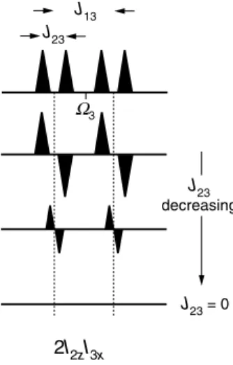
This is a somewhat involved topic which will only be possible to cover in outline here. 2I_2zI_3x Ω3 J₂₃ J₂₃ decreasing J₂₃ = 0 J₁₃

Illustration of how the intensity of an anti-phase multiplet decreases as the coupling which it is in anti-phase with respect to decreases. The in-phase multiplet is shown at the top, and below are three versions of the anti-phase multiplet for successively decreasing values of J₂₃.

7.6.1 One-dimensional spectra

Suppose that a 90°(y) pulse is applied to equilibrium magnetization resulting in the generation of pure x-magnetization which then precesses in the transverse plane with frequency Ω. NMR spectrometers are set up to detect the x- and y -components of this magnetization. If it is assumed (arbitrarily) that these components decay exponentially with time constant T₂ the resulting signals,

S t_x

( )

and S t_y

( )

, from the two channels of the detector can be written

S t_x

( )

=γ cosΩtexp

(

−t T₂

)

S t_y

( )

=γ sinΩtexp

(

−t T₂

)

where γ is a factor which gives the absolute intensity of the signal.

Usually, these two components are combined in the computer to give a complex time-domain signal, S(t)

S t S t iS t t i t t T i t t T x y

( )

=

( )

+

( )

=

₍

+

₎

(

−

)

=

_{( )}

(

−

)

γ γ

cos sin exp

exp exp Ω Ω Ω 2 2 [7.2]

The Fourier transform of S(t) is also a complex function, S(ω):

S FT S t A iD ω γ ω ω

( )

=

[ ]

( )

=

{

( )

+

( )

}

where A(ω) and D(ω) are the absorption and dispersion Lorentzian lineshapes:

A T D T T ω ω ω ω ω

( )

= −

(

)

+

( )

= −

(

)

−

(

)

+ 1 1 1 2 22 2 2 22 Ω Ω Ω

These lineshapes are illustrated opposite. For NMR it is usual to display the spectrum with the absorption mode lineshape and in this case this corresponds to displaying the real part of S(ω).

7.6.1.1Phase

Due to instrumental factors it is almost never the case that the real and imaginary parts of S(t) correspond exactly to the x- and y-components of the magnetization. Mathematically, this is expressed by multiplying the ideal function by an instrumental phase factor, φ_instr

S t

( )

=γ exp

(

iφ_instr

)

exp

( )

i tΩ exp

(

−t T₂

)

The real and imaginary parts of S(t) are

Re cos cos sin sin exp

Im cos sin sin cos exp

S t t t t T S t t t t T

( )

[ ]

=

(

−

)

(

−

)

( )

[ ]

=

(

+

)

(

−

)

γ φ φ γ φ φ instr instr instr instr Ω Ω Ω Ω 2 2

Clearly, these do not correspond to the x– and y-components of the ideal time-domain function.

The Fourier transform of S(t) carries forward the phase term

S

( )

ω =γ exp

(

iφ_instr

)

{

A

( )

ω +iD

( )

ω

}

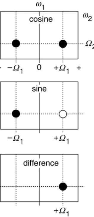
All modern spectrometers use a method know as quadrature d e t e c t i o n, which in effect means that both the x- and y -c o m p o n e n t s o f t h e magnetization are detected simultaneously.

Ω

ω ω

A b s o r p t i o n ( a b o v e ) a n d dispersion (below) Lorentzian l i n e s h a p e s , c e n t r e d a t frequency Ω.

The real and imaginary parts of S(ω) are no longer the absorption and dispersion signals: Re cos sin Im cos sin S A D S D A ω γ φ ω φ ω ω γ φ ω φ ω

( )

[

]

=

(

( )

−

( )

)

( )

[

]

=

(

( )

+

( )

)

instr instr instr instr

Thus, displaying the real part of S(ω) will not give the required absorption mode spectrum; rather, the spectrum will show lines which have a mixture of absorption and dispersion lineshapes.

Restoring the pure absorption lineshape is simple. S(ω) is multiplied, in the computer, by a phase correction factor, φ_corr:

S i i i A iD i A iD ω φ γ φ φ ω ω γ φ φ ω ω

( )

(

)

=

(

) (

)

{

( )

+

( )

}

=

(

(

+

)

)

{

( )

+

( )

}

exp exp exp

exp

corr corr instr

corr instr

By choosing φ_corr such that (φ_corr + φ_inst) = 0 (i.e. φ_corr = – φ_instr) the phase terms disappear and the real part of the spectrum will have the required absorption lineshape. In practice, the value of the phase correction is set "by eye" until the spectrum "looks phased". NMR processing software also allows for an additional phase correction which depends on frequency; such a correction is needed to compensate for, amongst other things, imperfections in radiofrequency pulses.

7.6.1.2Phase is arbitrary

Suppose that the phase of the 90° pulse is changed from y to x. T h e magnetization now starts along –y and precesses towards x; assuming that the instrumental phase is zero, the output of the two channels of the detector are

S t_x

( )

=γ sinΩtexp

(

−t T₂

)

S t_y

( )

= −γ cosΩtexp

(

−t T₂

)

The complex time-domain signal can then be written

S t S t iS t t i t t T i t i t t T i i t t T i i t t T x y

( )

=

( )

+

( )

=

₍

−

₎

(

−

)

−

( )

₍

+

₎

(

−

)

= −

( )

( )

(

−

)

=

( )

( )

(

−

)

γ γ γ γ φ

sin cos exp

cos sin exp

exp exp

exp exp exp

Ω Ω Ω Ω Ω Ω 2 2 2 2 exp

Where φ_{e x p}, the "experimental" phase, is –π/2 (recall that exp

( )

iφ =cosφ +isinφ, so that exp(–iπ/2) = –i).

It is clear from the form of S(t) that this phase introduced by altering the experiment (in this case, by altering the phase of the pulse) takes exactly the same form as the instrumental phase error. It can, therefore, be corrected by applying a phase correction so as to return the real part of the spectrum to the absorption mode lineshape. In this case the phase correction would be π/2.

S i A iD S D S A ω γ ω ω ω γ ω ω γ ω

( )

= −

( ) ( )

{

+

( )

}

( )

[

]

=

( )

[

( )

]

= −

( )

Re Im

Thus the real part shows the dispersion mode lineshape, and the imaginary part shows the absorption lineshape. The 90° phase shift simply swaps over the real and imaginary parts.

7.6.1.3Relative phase is important

The conclusion from the previous two sections is that the lineshape seen in the spectrum is under the control of the spectroscopist. It does not matter, for example, whether the pulse sequence results in magnetization appearing along the x- or y- axis (or anywhere in between, for that matter). It is always possible to phase correct the spectrum afterwards to achieve the desired lineshape.

However, if an experiment leads to magnetization from different processes or spins appearing along different axes, there is no single phase correction which will put the whole spectrum in the absorption mode. This is the case in the COSY spectrum (section 7.4.1). The terms leading to diagonal-peaks appear along the x-axis, whereas those leading to cross-peaks appear along y. Either can be phased to absorption, but if one is in absorption, one will be in dispersion; the two signals are fundamentally 90° out of phase with one another.

7.6.1.4Frequency discrimination

Suppose that a particular spectrometer is only capable of recording one, say the

x-, component of the precessing magnetization. The time domain signal will then just have a real part (compare Eqn. [7.2] in section 7.6.1)

S t

( )

=γ cosΩtexp

(

−t T₂

)

Using the identity cosθ = 1

(

exp

( )

θ +exp

( )

− θ

)

2 i i this can be written

S t i t i t t T i t t T i t t T

( )

=

[

( )

+

(

)

]

(

−

)

=

( )

(

−

)

+

(

)

(

−

)

1 2 2 1 2 2 12 2 γ γ γ

exp exp – exp

exp exp exp – exp

Ω Ω