1 2 3 4 5 6 7 8 9 10 11 12 13 14 15 16 17 18 19 20 21 22 23 24 25 26 27 28 29 30 31
Sub
‐
arctic
and
Arctic
sea
surface
temperature
and
its
relation
to
ocean
heat
content
1982
‐
2010
Submitted November 19, 2011 Revised January 27, 2012
Gennady A. Chepurin and James A. Carton
Corresponding author: Gennady Chepurin ([email protected]) Department of Atmospheric and Oceanic Science
33 34 35 36 37 38 39 40 41 42 43 44 45 46 47 48 49 50 51 52 53 Abstract
This is an examination of SST variability in the Subarctic and Arctic during the 29 year period 1982-2010, based primarily on data from the Pathfinder AVHRR data set as well as operational SST products from NOAA and the UK Meteorological Office. A goal is to explore the
connection between SST variations in the subpolar gyres and SST variations further north, with emphasis on the Nordic Seas because of their atmospheric exposure and connection to the overturning circulation. After identifying and correcting for biases in Pathfinder AVHRR (also present in the operational products) the seasonal cycle and 29-year warming trend is described. The analysis shows that much of the warming of the North Atlantic subpolar gyre during the period occurred in 1990s and compensated the earlier cooling during the decades of the early 1960s to mid-1990s in this same region.
Superimposed on this warming trend the analysis reveals a succession of residual SST anomalies with 0.5oC amplitudes that seem to move out of the North Atlantic subpolar gyre into the Nordic Seas following the North Atlantic and Norwegian Currents. Within the Nordic Seas these SST anomalies slowly advect in a counterclockwise direction. After approximately six years part of the anomalies exit the Nordic Seas through the East Greenland Current. The connection between these SST anomalies and underlying anomalies of 0/300m heat content is discussed. The
existence of these SST anomalies and their origin at lower latitudes highlights the importance of ocean exchanges in influencing Arctic climate.
54 55 56 57 58 59 60 61 62 63 64 65 66 67 68 69 70 71 72 73 74 75 1. Introduction
This study uses the multi-satellite Pathfinder V5 Advanced Very High Resolution (AVHRR) SST data set in the Subarctic and Arctic Ocean to examine interannual to decadal variability of SST during 1982-2010. Recent modeling studies have shown that atmospheric circulation has enhanced sensitivity to SST anomalies at high latitude with positively correlated cyclonic surface winds and an anticyclonic response at 300mb (Deser et al, 2007; Hawkins and Sutton, 2009; 2011). Yet documentation of the SST anomalies that might drive these changes in circulation, and the connection of the SST anomalies to oceanic changes further equatorward is limited. This study is an attempt to fill this gap through examination of the uniquely large, well-calibrated Pathfinder SST product along with available in situ observations.
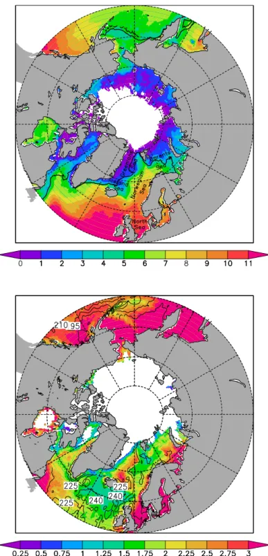
The SST anomalies of interest to us are superimposed on a geographically variable time mean and seasonal pattern of SST variability. Poleward of 50oN Pathfinder SST has its highest annual average values along the European side of the North Atlantic, extending northwards into the Norwegian Sea (Fig. 1 upper panel). In these regions annual average temperatures generally exceed 8oC. In contrast, the coldest temperatures at these latitudes are evident on the western side of the Nordic Seas and on the margins of the southern Labrador Sea (typically uncovered by wintertime sea ice), with temperatures generally below 2oC. SST in the Bering Sea region of the Pacific sector lies between these two extremes, in the range of 3-7oC. Further poleward
Pathfinder SST is only available in summer, and during that season it frequently has values cooler than 1oC. The seasonal cycle of SST in our domain of interest is dominated by its annual
varying amplitude. The largest amplitudes, exceeding 4oC (RMS climatological monthly variability >3oC), are evident in the shallow Bering, North, and Barents Seas (Fig. 1 lower panel). 77 78 79 80 81 82 83 84 85 86 87 88 89 90 91 92 93 94 95 96 97 98 99
Superimposed on the seasonal cycle, SST exhibits anomalies with interannual to multi-decadal timescales and basin-scale structure that are a prominent feature of the wintertime North Atlantic Ocean. Stationary empirical orthogonal eigenfunction analyses of these SST anomalies show two dominant stationary patterns. The first, according to Deser and Blackmon (1993), is a broad cooling and warming of the basin which varies on multi-decadal timescales (see also Rayner et al., 2003). Reminiscent of this, basin-scale warming has been a feature of the North Atlantic since the 1970s. The second is an interannually varying pattern in which SST anomalies at 50oN vary in opposite phase to those in the subtropics. This pattern can be viewed as part of a tripole pattern of SST that shows up in many diagnostic studies (e.g. Wallace et al., 1990; Kushnir, 1994). Observational and modeling studies suggest that this tripole pattern of SST is the ocean’s response to the North Atlantic Oscillation (NAO) pattern of sea level pressure gradient, and an associated meridional fluctuation of the position of winter storm tracks (Deser and Blackmon, 1993). During the decades of the early 1960s to mid-1990s a rise of the winter Index of the NAO was associated with anomalously warm SSTs in the subtropics and cool SSTs in the subpolar gyre. Since the mid-1990s the Index has been in steady retreat to below normal conditions.
In addition to these stationary patterns, observational and modeling studies by Hansen and Bezdek (1996), Sutton and Allen (1997), and Krahmann et al. (2001) point to the existence of
0.5-1oC SST anomalies that drift along the Gulf Stream and North Atlantic Current into the subpolar gyre with slow speeds of ~2 cm s-1. Comparison of SST and subsurface temperature shows these anomalies extend vertically through the upper thermocline. These studies do not trace the movement of the anomalies past their presence in the subpolar gyre, leaving open any question of their connection to ocean variability further north.
100 101 102 103 104 105 106 107 108 109 110 111 112 113 114 115 116 117 118 119 120 121
Within the subpolar gyre and Nordic Seas on similar timescales Venegas and Mysak (2000) found evidence of anomalies of sea ice concentration, while Furevik (2000) identified patterns of anomalous SST in the NOAA operational SST product that seem to form off Scotland then move northward. Furevik’s SST anomalies seem to follow the Norwegian Atlantic Current, with its complement of Atlantic Water from the North Atlantic Current (Orvik and Niiler, 2002), around Nordic/Barents Seas, eventually exiting southward through the East Greenland Current. Studies of subsurface temperature in the Nordic Seas suggest that the SST anomalies tracked by Furevik extend vertically and thus are dynamically related to movements of Atlantic Water (Dmitrenko et al., 2009; Carton et al., 2011). In this study we revisit the historical record of satellite infrared SST, document variability of SST at subpolar latitudes and attempt to connect SST variability, mainly in the Atlantic sector, to variability further poleward through examination of remotely sensed SST.
Our primary SST data set is constructed using an empirical quasi-linear relationship between SST and brightness temperature measurements from seven satellites in two infrared 11-12 µm channels (channels 4 and 5) (Kilpatrick et al., 2001). This Pathfinder v5 algorithm uses the
123 124 125 126 127 128 129 130 131 132 133 134 135 136 137 138 139 140 141 142 143 144
atmospheric absorption of infrared emissions, most notably by water vapor. This approach works well at lower latitudes with high column water vapor and leads to a global average (60o S-60oN) nominal SST error of 0.5oC (Donlon, 2009). However, in the dry, cold conditions at high latitudes the problem of estimating SST from infrared brightness temperature becomes more difficult. Vincent et al. (2008a,b) show that there channel 4-5 brightness temperature difference is no longer a good proxy for column water vapor. Also, the prevalence of low level clouds, haze, and ice fog throughout much of the year makes removal of cloud-contaminated pixels both important and difficult (Barton, 1995; Key et al., 1997; Chen et al., 2002; Shupe, 2010). A corresponding record of SST using longer wavelength microwave sensing is less sensitive to cloud contamination, but is only available since 2002. Additional problems are caused by emissions from the sea ice near the marginal ice zone, as well as by emission from sub-pixel-sized sea ice in the open water (Reynolds et. al., 2007).
It is thus not surprising that comparison to in situ observations by Steele (2008) suggest the presence of biases in the range of 0.2-0.8oC and RMS errors of 1oC while the satellite-in situ comparison of Vincent et al (2008a) at a single station within a polynya surrounded by pack ice suggests the errors may be even larger. Because of these concerns about the accuracy of the primary SST data set we begin by comparing the Pathfinder SST to available in situ temperature profile observations and to alternative analyses. A goal of this comparison is to contribute to an understanding of the characteristics of Pathfinder v.5 SST at high latitudes.
145 146 147 148 149 150 151 152 153 154 155 156 157 158 159 160 161 162 163 164 165 166 167
The primary SST data set used in this study is the 4km resolution AVHRR satellite-based Pathfinder v. 5.0/5.1 SST (Kilpatrick, et al., 2001). This product combines infrared radiance measurements from seven NOAA polar orbiting satellites. Satellites were in sun-synchronous orbits with 14+ orbits per day and an ascending pass occurring between 13:30 and 14:20 local time (except NOAA 17). Three satellites, NOAA 6, NOAA 11, and NOAA 14 are known to have instrument problems (Kilpatrick et. al., 2001; Podesta et. al., 2003) that need to be accounted for in the Pathfinder data set. In this study we use L3 data (in which the data is gridded, but no attempt is made to fill missing pixels) eliminating pixels with possible cloud or sea ice contamination (highest flag setting). The data is then monthly averaged and re-binned onto a nominal 0.5ox0.5o grid poleward of 50oN to increase our confidence and reduce the incidence of missing data. To reduce the possibility of a near-surface heating effect we use only the data contained in the “nighttime” Pathfinder files. For most satellites except NOAA17 the nighttime observations correspond to around 2am. For NOAA17 the nominal time is closer to 10pm.
Because of concerns about bias due to processes described in the Introduction we compare the monthly-averaged Pathfinder SST to all available collocated in situ temperature observations from the hydrographic data set of Carton et al. (2011) at their uppermost depth within the top 10m, binned into a 1ox1o horizontal grid and also monthly averaged (Fig. 2). This hydrographic data set contains all in situ temperature and salinity measurements in the National Oceanographic Data Center (Boyer et al, 2009; extracted January, 2011) combined with profile observations from the International Council of the Exploration of the Seas database, the Woods Hole Oceanographic Institution Ice-Tethered Profile data set, the North Pole Environmental
168 169 170 171 172 173 174 175 176 177 178 179 180 181 182 183 184 185 186 187 188 189
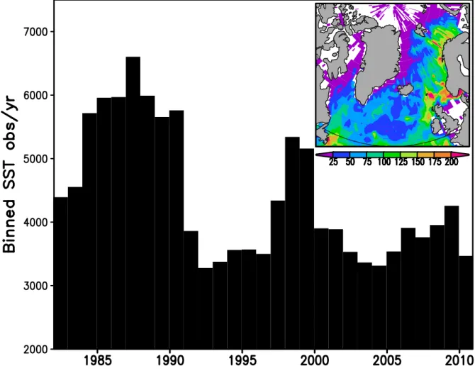
Observatory data set, and the Nansen and Amundsen Basin Observational System data set. This data set includes a minority of observations collected using Expendable Bathythermographs and these have been bias-corrected following Levitus et al. (2009). The total number in situ near-surface temperature observations during 1982-2010, after binning into 1ox1oxmo bins is: 128,243. The coverage is heaviest during the decade of the 1980s, peaking at 19,000 in 1987, and is geographically concentrated in the region poleward of Scandinavia and the Kola
Peninsula.
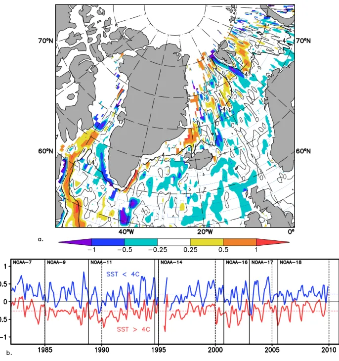
The collocated time mean difference between Pathfinder and in situ SST shows indeed that Pathfinder is too cold by 0.35oC in regions where SST is warmer than 4oC (Fig. 3 upper panel). A similar cool bias was identified by Reynolds et al. (2007) which they attribute to low level cloud contamination. However, the unexpected aspect of our comparison is that the sign of the bias changes over water cooler than 4oC. There, we find Pathfinder is too warm by 0.25oC-1oC. Both cool and warm biases persist throughout our period of interest, but vary in amplitude as the source of the SST data shifts from one satellite to another (Fig. 3 lower panel). Interestingly, the most recent satellite, NOAA 18, has significantly reduced bias compared to earlier satellites.
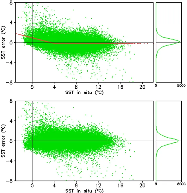
The temperature-dependence of the bias in AVHRR is evident in a plot of collocated SST differences versus in situ SST (Fig. 4 upper panel). Since we lack theoretical understanding of the causes of this Pathfinder SST bias we propose a simple piecewise linear SST-dependent correction as follows:
C SST C SST C SST o path o path o 4 4 205 . 0 SST C 0.875 -SST * 1.27 path o path (1 190 191 192 193 194 195 196 197 198 199 200 201 202 203 204 205 206 207 208 209 210
After applying this empirical bias correction the resulting collocated SST differences lie in the range of ±2.5oC with an RMS difference of 1oC, a value twice the size of the expected global average uncertainty (Donlon et al., 2009). The larger uncertainty at high latitudes reflects the greater challenges of remotely sensing SST there (Fig. 4 lower panel). The corrected Pathfinder data set used throughout the rest of this study consists of 348 monthly bias-adjusted fields with a minimum spatial resolution of 40km.
Below we compare our Pathfinder SST with the monthly averages of two operational SST products that span our period of interest: the NOAA optimal Interpolation SST v.2 (OI-V2, Reynolds et al., 2007), and the UK Meteorological Office Operational Sea Surface Temperature and Sea Ice Analysis (OSTIA, Stark et al., 2007). OI-V2, available daily at 0.25ox0.25o
resolution, combines AVHRR SST with microwave SST since 2002 and includes a bias adjustment algorithm equatorward of 60oN to improve agreement with in situ observations at these latitudes. To mask out regions obscured by sea ice we have used the delayed sea ice concentration estimated by Cavalieri et al. (1999) for the period through December 2004 and have continued past that date with the sea ice concentration estimates from real-time microwave satellite data by Grumbine (1996) to mask those grid points where sea ice was observed more than 30% of the time for both Pathfinder and OI-V2 products.
211 212 213 214 215 216 217 218 219 220 221 222 223 224 225 226 227 228 229 230 231 232
OSTIA, available daily at even finer 0.05°x0.05° resolution, combines Pathfinder AVHRR with EnviSat infrared and other microwave measurements, eliminating daytime observations collected under low wind conditions to limit possible diurnal skin effects. As in the case of OI-V2, in situ observations are included in the OSTIA processing as part of a bias-correction scheme. The ice mask used in OSTIA is provided by the European Organization for the Exploitation of
Meteorological Satellites (EUMETSAT) Ocean and Sea Ice Satellite application Facility.
Our comparison of three satellite SST products (partially shown in fig.6) reveals that these three data sets are very similar in the Arctic. This similarity is to be expected because of the
importance of the AVHRR and the limited number of in situ observations (Hoyer et al., 2011). Microwave SST observations are also included in OI-V2 and OSTIA but have higher
measurement error and are only available in recent years (Hoyer et al., 2011). Differences between OI-V2 and OSTIA likely result from a variety of sources including the differing ways in which in situ observations impact the analyses, differing ice masks, differing cloud clearing algorithms, and differences in gridding algorithms.
The in situ profile observations are vertically integrated to estimate heat content. For this part of the study we have chosen to compute heat content over the upper 300m. This depth has been chosen to be sufficiently shallow to be appropriate for such shallow areas as the Barents Sea (average depth 230m) and Fram Strait, but deep enough to sample key water masses in the Nordic Seas. In the Nordic Seas there are two water masses of particular interest, the warm and salty Atlantic Water, which is several hundred meters thick and very homogenous (Carton et al.,
233 234 235 236 237 238 239 240 241 242 243 244 245 246 247 248 249 250 251 252 253 254
2011), and cold, fresh Polar Water flowing southward through Fram Strait at depths 0-150 meters (Jones et al., 2008).
3. Results
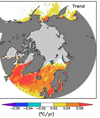
Over much of the 20th century the subpolar gyre stands out from the rest of the Atlantic by exhibiting a slow -0.5oC/100yr cooling trend (e.g., Deser et al., 2010). In contrast, our 29 year SST data set documents a reversal of this trend in the subpolar gyre and its replacement by rapid warming at a rate in excess of 0.6oC/10yr (Fig. 5 left). This warming trend extends into the Nordic Seas where it still exceeds 0.3oC/10yrs. Much of this warming of SST in the subpolar gyre occurred in the mid-1990s so that SST in the second half of the decade is more than 1oC warmer than SST in the first half of the decade (Fig. 5 right). The warming in the 1990s is also evident in the subpolar North Pacific, and is evident in both seasonal and annual analyses (only the annual trend is shown). While this warming occurred coincident with a change in satellites (from NOAA11 to NOAA14); comparison to in situ SST observations (Fig. 3 lower panel) reassures us that the warming was not due to a change in satellite sensors. Indeed, it seems likely that an important aspect of the warming in the 1990s is the constructive interference of tripole like North Atlantic decadal (e.g. Wallace et al., 1990; Kushnir, 1994) and broad North Atlantic multi-decadal (Deser and Blackmon, 1993) patterns of surface climate in this basin, reviewed in the Introduction.
To focus on the SST anomalies relative to the multi-decadal SST pattern we subtract the trend (shown in Fig. 5 for Pathfinder) from the SST anomalies at each grid point after removing the
255 256 257 258 259 260 261 262 263 264 265 266 267 268 269 270 271 272 273 274 275 276 277
seasonal cycle to create residual SST anomaly data sets for each product. The rest of this section focuses on the characteristics of these 0.3-1.3oCresidual anomalies of SST (RMS variability remaining after the climatological monthly cycle is removed, is presented in Fig. 6, lefthand panels).
We begin by examining the spatial structure of the residual SST as it appears in the three
products. At latitudes between 50o-60oN the highest levels of variability in Pathfinder SST occur on the western side of the North Atlantic and south of Greenland with values of around 1oC. Variability is less than 0.5oC in the southern part of the Nordic Seas, increasing again further north, extending into the Barents Sea. These patterns of variability are similar for the other two SST products, although with somewhat lower amplitudes. The lower interannual variability in OI-V2 and OSTIA is likely due to the smoothing inherent in their construction. The similarity of the SST residuals for the three products is not just reflected by the similarity of spatial structures of SST variability, but also by mutual correlations that fall in the range 0.85-0.95 (Fig. 6
righthand panels). The regions that are exceptions to this close agreement are: the southern Labrador Sea, the Sea of Okhotsk and near the Aleutian Islands. It is reassuring that no change in OI-V2 SST variability or its agreement with Pathfinder is evident at 60oN, the latitude poleward of which OI-V2 bias correction is eliminated.
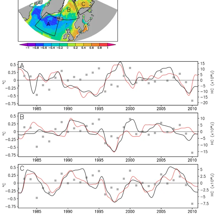
We next examine the evolution of SST residuals by examining their time series area-averaged in three regions in the North Atlantic and Nordic Seas (Fig. 7 middle and lower). The subpolar North Atlantic region (45o-20oW, 52o-65oN) we designate Region A, the western Nordic Seas (20oW-15oE, 65o-79oN) we designate Region B, while the Barents Sea (18o-55oE, 67o-78oN) we
278 279 280 281 282 283 284 285 286 287 288 289 290 291 292 293 294 295 296 297 298 299
treat separately as Region C. Even with this area-averaging and 2-year time-smoothing the Pathfinder data has too many missing pixels to produce reliable time series in these three regions. However, we can exploit the good agreement between Pathfinder and OI-V2 (e.g. Fig. 6) and substitute the latter product into this comparison (the results are very similar when we use OSTIA).
The SST anomaly time series for Region A has 0.5oC amplitude variations, with warm anomalies in the late-1980s, late-1990s, and mid-2000s and cool anomalies in the early 1990s. Regions B and C have rather similar time series with warm SSTs in the early to mid-1980s and early 1990s, and anomalously cool SSTs in the late-1990s (somewhat later in C than B). Since 2000 the correspondence of interannual SST variability between B and C is less evident. The successive appearance of cool SST in region A in the early 1990s, in regions B and C in the late 1990s, and a similar succession of other warm and cool SST anomalies suggests the possibility that
anomalies are propagating from Region A to Regions B and C.
We next evaluate the vertical extension of the residual SST anomalies by comparing the regional time series to corresponding time series of heat content anomalies. It is striking that SST in these regions is quite well correlated with heat content with a zero lag correlation of 0.68 in the
western Nordic Seas and with even higher correlations in the subpolar gyre and Barents Sea. These high correlations between surface and subsurface temperature, which seem consistent with previous studies in the subpolar gyre and Nordic Seas mentioned in the Introduction suggest that the SST anomalies are being advected by the North Atlantic Current into the Nordic Seas.
300 301 302 303 304 305 306 307 308 309 310 311 312 313 314 315
In light of this result we revisit theconnection between SST propagation in the North Atlantic and propagation in the Nordic Seas by computing the time lagged correlation at one year
intervals of interannually varying SST. We take as our focus the geographic location of Atlantic Water within the Nordic Seas north of 70oN (defined by the region with salinity higher than 35psu at the 100m depth) (this Atlantic Water Zone [AWZ], enclosed by a solid black contour, is shown in all panels of Fig. 8). The lag correlation reveals that warm residual SST anomalies covering the AWZ are preceded four years earlier by anomalously warm SSTs in the subpolar North Atlantic and anomalously cold SSTs in the Greenland and Barents Seas. Warm residual SST anomalies in the North Atlantic gradually shift eastward to the southern Norwegian Sea and northern North Sea region. Then these anomalies move northward along the coast of Norway.
If advected by ocean currents, this northward movement will take place in the Norwegian Atlantic Current and Norwegian Coastal Current. Of these, the Norwegian Coastal Current is close to the coast and more than twice as fast (Mork and Skagseth, 2009). The SST anomalies move in the Norwegian Sea from the Faroe Island to the Fram Strait ~2-3 years. The average speed of propagation SST anomalies is 2.70.6cm/s. It is in reasonable agreement with the speed of propagation in the Norwegian Sea estimated from temperature and salinity observations on hydrographic sections by Holliday et al. (2008) and Skagseth et al. (2008). The zero lag correlation shows that anomalously warm SSTs in the AWZ are associated with anomalously cool SSTs in the western subpolar North Atlantic. One to two years later this cold anomaly has shifted northeastward into the Norwegian and Barents Seas.
316 317 318 319 320 321 322
323 324 325 326 327 328 329 330 331 332 333 334 335 336 337 338 339 340 341 342 343 344
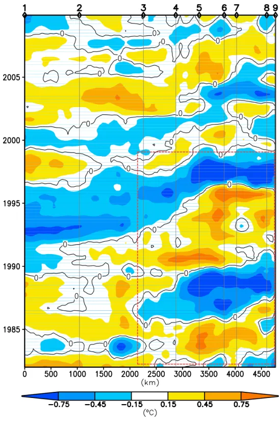
The shift of the lag correlation allows us to define the average path of these SST anomalies, indicated by a dashed line on the panels of Fig. 8, with station numbers to indicate the approximate 12 month movement of the anomalies. The time evolution of residual SST
anomalies along this path is presented in Fig. 9 (the station numbers are reproduced along the top of the figure). For many of these residual SST anomalies in the later 1980s and 1990s the figure seems to be consistent with advection along this path. However we note that some anomalies such as the warm anomaly in the mid-2000s seem to appear nearly simultaneously throughout the subpolar gyre to the Norwegian coast (stations 1-4). This more rapid propagation in the recent decade maybe connected with the northward shift of the North Atlantic Current documented by Hakkinen and Rhines (2009) in surface drifter data.
Finally, we revisit the connection between these residual SST anomalies and the basin-scale meteorology -- primarily to aspects of surface meteorology associated with the North Atlantic Oscillation. Such a connection has been suggested for example by Deser and Blackmon (1993). Comparison of the time series of residual SST in the subpolar gyre (Region A) shows the
expected result that residual SST anomalies in this region, the northern extension of the SST tripole, is negatively correlated with the NAO Index (Wallace and Gutzler,1981, and
ftp://ftp.cpc.ncep.noaa.gov/wd52dg/data/indices/nao_index.tim) with correlations of -0.6 (Fig. 7). Further north in the Nordic Seas residual SST becomes positively correlated to NAO. An example of this positive relationship is the cooling of SST in the mid-1990s, which occurred when the NAO Index was in its negative phase. However, the reader is reminded that a linear trend has been removed from all variables. If this trend were not removed the correlations would
be much lower since the past decade has been one of dramatically warming SST in the Nordic Seas, but declining NAO Index.
345 346 347 348 349 350 351 352 353 354 355 356 357 358 359 360 361 362 363 364
4. Summary and Discussion
Recent dramatic changes in Arctic air temperature and sea ice coverage have brought increasing attention to the question of changes in other climate variables. This study is a reexamination of the variability of SST in the Subarctic and Arctic during our 29-year period of interest 1982-2010 during which AVHRR infrared observations are available. This study exploits the efforts of the GODAE1 High Resolution SST Pilot Project to recalibrate and match observations from a succession of seven NOAA polar orbiting satellites. Our brief comparison of this product to in situ surface temperature observations shows the presence of a -0.35oC cool bias in water with temperatures above 4oC, consistent with previous studies by Vincent et al (2008a,b).
Unexpectedly we also find enhanced scatter and a warm bias of up to 1oC in regions of cooler temperatures that are also close to the edges of the sea ice. Correcting for these biases gives an RMS difference (satellite minus in situ) of monthly averaged SST of approximately 1oC, but with occasional positive outliers for which the differences may be much larger. We also compare the Pathfinder AVHRR to two operational SST products, OI-V2 and OSTIA, and find strong similarity among them. This result is understandable because both of the operational products incorporate AVHRR.
1
365 366 367 368 369 370 371 372 373 374 375 376 377 378 379 380 381 382 383 384 385 386
We present a general description of SST in this region with emphasis on the Atlantic sector because of its importance for climate and since the ice-free portion of this sector extends to polar latitudes even in winter and thus remains visible from space. We begin by examining the
seasonal cycle and show that SST has its maximum in late July and early August in the subpolar North Pacific and Bering Sea and roughly two weeks later in the subpolar North Atlantic and Nordic Seas. The amplitude of the seasonal cycle exceeds 4oC in the North Pacific and the shallow North and Barents Seas in the Atlantic sector. The data coverage is insufficient to detect any significant shift in the phase or amplitude of the seasonal cycle during our period of interest.
Superimposed on this strong seasonal cycle is a striking decadal warming trend that is most pronounced in the North Atlantic subpolar gyre. Much of this warming occurred during the decade of the 1990s and in that one decade the warming compensated for a weak cooling reported in previous decades in the subpolar gyre. Here we show that the resulting warming of the subpolar gyre extends poleward through the Nordic Seas. We note that this decade was also characterized by a substantial decrease in the NAO Index, indicating a southward shift in winter of the location of the atmospheric storm tracks. Removing the linear trend from our data set, we find a negative relationship between subpolar SST and the NAO Index, consistent with a number of previous studies examining in situ temperature records.
After removal of the seasonal cycle and the linear trend the residual anomalous SST reveals decadal variations in both the North Atlantic and the Nordic Seas. Within the North Atlantic, advections of SST anomalies by the Gulf Stream/North Atlantic Current have been discussed in
attention except for the study by Furevik (2000), and their origin is still not clear. The results shown here strongly suggest that a significant part of the decadal variability of SST in the Nordic Seas results from the slow advection of surface and subsurface temperature anomalies into the Nordic Seas along the North Atlantic Current. Once in the Nordic Seas the anomalous water masses advect around the Nordic Seas, with part of the anomaly exiting southward through the East Greenland Current and part continuing northeastward through the Barents Sea. If so, this result provides further evidence of dynamical coupling between the ocean basins and, because of its impact on basal melt, raises interesting possibilities for interaction with the sea ice coverage and the overlying atmospheric circulation.
388 389 390 391 392 393 394 395 396 397 398 399 400 401 Acknowledgements
GAC and JAC gratefully acknowledge support from the NASA Oceans Program
(NNX09AF33G). The hydrographic observation set was provided by Mr. James Reagan of the NOAA National Oceanographic Data Center.
References 402 403 404 405 406 407 408 409 410 411 412 413 414 415 416 417 418 419 420 421
Barton, I. J. (1995), Satellite-derived sea surface temperatures: Current status. J. Geophys. Res., 100, 8777–8790, doi:10.1029/95JC00365.
Boyer, T. P., J. I. Antonov, O. K. Baranova, H. E. Garcia, D. R. Johnson, R. A. Locarnini, A. V. Mishonov, D. Seidov, I. V. Smolyar, and M. M. Zweng (2009), World Ocean Database 2009, Chapter 1: Introduction, NOAA Atlas NESDIS 66, Ed. S. Levitus, U.S. Gov. Printing Office, Wash., D.C., 216 pp., DVD.
Carton, J.A., G.A. Chepurin, J. Reagan, and S. Häkkinen (2011), Interannual to Decadal
Variability of Atlantic Water in the Nordic and Adjacent Seas, J. Geophys. Res.-Oceans, in press.
Cavalieri, D. J., C. L. Parkinson, P. Gloersen, J. C. Comiso, and H. J. Zwally (1999), Deriving long-term time series of sea ice cover from satellite passive-microwave multisensor data sets. J. Geophys. Res., 104, 15 803–15 814.
Chen, Y., J.A. Francis, and J.R. Miller (2002), Surface Temperature of the Arctic: Comparison of TOVS Satellite Retrievals with Surface Observations, J. Clim., 15, 3698-3708. Deser, C., R.A. Tomas, and S. Peng (2007), The transient atmospheric circulation response to
North Atlantic SST and sea ice anomalies, J. Clim., 20, 4751-4767.
Deser, C., A. S. Phillips, and M. A. Alexander (2010), Twentieth century tropical sea surface temperature trends revisited, Geophys. Res. Lett., 37, L10701,
422 423 424 425 426 427 428 429 430 431 432 433 434 435 436 437 438 439 440 441 442
Donlon, C.J., K.S. Casey, I.S. Robinson, et al. (2009), The GODAE High-Resolution Sea Surface Temperature Pilot Project. Oceanography, 22, 34–45,
doi:10.5670/oceanog.2009.64.
Dmitrenko, I.A., D. Bauch, S. A.Kirillov, N. Koldunov, P.J. Minnett, V.V. Ivanov,
J.A.Holemann, and L.A.Timokhov (2009), Barents Sea upstream events impact the properties of Atlantic water inflow into the Arctic Ocean: Evidence from 2005 to 2006 down stream observations, Deep-Sea Res. I, 56, 513–527.
Furevik, T. (2000), On anomalous sea surface temperatures in the Nordic Seas, J. Clim., 13, 1044– 1053.
Grumbine, R. W. (1996), Automated passive microwave sea ice concentration analysis at NCEP. NOAA Tech. Note 120, 13pp. [Available from NCEP/NWS/NOAA, 5200 Auth
Road,Camp Springs, MD 20746.]
Hakkinen, S., and P. B. Rhines (2009), Shifting surface currents in the northern North Atlantic Ocean , J. Geophys. Res., 114, C04005, doi:10.1029/2008JC004883
Hansen, D.V., and H.F. Bezdek (1996), On the nature of decadal anomalies in North Atlantic sea surface temperature, J. Geophys. Res., 101, 8749-8758.
Hawkins, E., and R. Sutton (2009), Decadal predictability of the Atlantic Ocean in a coupled GCM: forecast skill and optimal perturbations using linear inverse modeling, J. Clim., 22, 3960-3978.
Hawkins, E., and R. Sutton (2011), Estimating climatically relevant singular vectors for decadal predictions of the Atlantic Ocean, J. Clim., 24, 109-123.
443 444 445 446 447 448 449 450 451 452 453 454 455 456 457 458 459 460 461 462 463 464
Hoeyer, J. L., I. Karagali, R. Tonboe, G. Dybkjær (2011), Multi sensor validation and error characteistics of Arctic satellite sea surface temperature observations, Proceedings from 12th GHRSST, p. 221, Science Team meeting, Edinburgh, GB.
Holliday, N. P., S. L. Hughes, S. Bacon, A. Beszczynska-Moller, B. Hansen, A. Lavin, K. A. Mork, S. Osterhus, T. Shverwin, and W. Walczowski, (2008), Reversal of the 1960s to 1990s freshening trend in the northeast North Atlantic and Nordic Seas., Geophys. Res., Letts, 35, L03614, doi:10.1029/2007GL032675.
Jones, E., L. Anderson, S. Jutterstrom, J. Scott (2008), Sources and distribution of fresh water in the Eastern Greenland Current, Progress in Oceanography,78, 37
(doi:10.1016/j.pocean.2007.06.003)
Key J.R., J.B. Collins, C. Fowler, and R.S. Stone (1997), high latitude surface temperature estimates from thermal satellite data, Remote Sens. Environ., 61, 302-309.
Kilpatrick, K. A., G. P. Podesta, and R. Evans (2001), Overview of the NOAA/NASA Pathfinder algorithm for sea surface temperature and associated matchup database, J. Geophys. Res.,
106, 9179–9197.
Krahmann, G., M. Visbeck, and G. Reverdin (2001), Formation and propagation of temperature anomalies along the North Atlantic Current, J. Phys. Oceanogr., 31, 1287-1303.
Kushnir, Y. (1994), Interdacadal variations in North-Atlantic sea-surface temperature and associated atmospheric. J. Clim., 7, 141-157.
Levitus S., J.I. Antonov, T.P. Boyer, R.A. Locarnini, H.E. Garcia, and A.V. Mishonov (2009), Global ocean heat content 1955-2008 in light of recently revealed instrumentation problems, Geophys. Res., Letts., 36, L07608.
465 466 467 468 469 470 471 472 473 474 475 476 477 478 479 480 481 482 483 484
Mork, K. A., and O. Skagseth, (2009) Volume, heat, and freshwater fluxes toward the Arctic from combined altimetry and hydrography in the Norwegian Sea, Ocean Sci. Discuss., 6, 2357-2388.
Orvik, K.A., and P. Niiler (2002), Major pathways of Atlantic water in the northern North Atlantic and Nordic Seas toward Arctic, Geophys. Res. Letts., 29, 1896,
doi:10.1029/2002GL015002.
Podesta, G.P., M. Arbelo, R. Evans, K. Kilpatrick, V. Halliwell, and J. Brown (2003), Errors in high-latitude SSTs and other geophysical products linked to NOAA-14 AVHRR channel 4 problems, Geophys. Res. Letts., 30, 1548, doi:10.1029/2003GL017178.
Rayner, N. A., et al. (2003), Global analyses of sea surface temperature, sea ice, and night marine air temperature since the late nineteenth century, J. Geophys. Res., 108, 4407, doi:10.1029/2002JD002670.
Reynolds, R.W., T.M. Smith, C. Liu, D.B. Chelton, K.S. Casey, and M.G. Schlax, (2007), Daily high-resolution-blended analyses for sea surface temperature, J. Clim., 20, 5473-5496.
Shupe, M.D., 2011. Clouds at Arctic Atmosphere Observatories, Part II: Thermodynamic phase characteristics. J. Appl. Meteor. Clim., accepted.
Skagseth, O., T. Furevik, R. Ingvaldsen, H. Loeng K. A. Mork, K. A. Orvik, and V. Ozhigin, (2008), Volume and heat transports to the Arctic Ocean via the Norwegian and Barents Seas, pp. 45–64 in Arctic-Subarctic Ocean Fluxes. R.R. Dickson, J. Meincke, and P. Rhines, eds, Springer, Dordrecht.
485 486 487 488 489 490 491 492 493 494 495 496 497 498 499 500 501 502 503 504
Stark, J.D. C.J. Donlon, M.J. Martin, and M.E. McCulloch (2007), OSTIA : An operational, high resolution, real time, global sea surface temperature analysis system. Oceans '07 IEEE Aberdeen, conference proceedings.
Steele, M., W. Ermold, and J. Zhang (2008), Arctic Ocean surface warming trends over the past 100 years, Geophys. Res. Letts., 35, L02614, doi:10.1029/2007GL031651.
Sutton, R.T., and M.R Allen (1997), Decadal predictability of North Atlantic sea surface temperature and climate, Nature, 388, 563-7.
Venegas, S.A., and L.A. Mysak (2000), Is There a Dominant Timescale of Natural Climate Variability in the Arctic? J. Clim., 13, 3412-3434.
Vincent, R. F., R. F. Marsden, P. J. Minnett, K. A. M. Creber, and J. R. Buckley (2008a), Arctic waters and marginal ice zones: A composite Arctic sea surface temperature algorithm using satellite thermal data, J. Geophys. Res., 113, C04021, doi:10.1029/2007JC004353. Vincent, R.F., R.F. Marsden, P.J. Minnett, and J. R. Buckley (2008b), Arctic waters and
marginal ice zones: 2. An investigation of arctic atmospheric infrared absorption for advanced very high resolution radiometer sea surface temperature estimates, J. Geophys. Res., 113, C08044, doi:10.1029/2007JC004354.
Wallace, J. M., and D. S. Gutzler (1981), Teleconnections in the geopotential height field during the Northern Hemisphere winter, Mon. Wea. Rev., 109, 784-812.
Wallace, J. M., Smith, C., and Jiang, Q. R., (1990), Spatial patterns of atmosphere ocean interaction in the northern winter. J. Clim., 3, 990-998.
Figure legends 505 506 507 508 509 510 511 512 513 514 515 516 517 518 519 520 521 522 523 524 525 526
Figure 1. Time mean (oC, upper panel) and climatological monthly Pathfinder SST variability (lower panel). White area in upper panel is free from the ice less one full month per year. North of the bold black line in upper panel and under the white area in lower panel sea ice was
observed more than 30% of the time. RMS variability of the twelve climatological monthly average SST fields (oC, colors) and year day of maximum of the annual harmonic (contours) is shown in lower panel.
Figure 2. In situ SST observation coverage with time in the domain 50oN-90oN, 90oW-60oE binned into 1ox1ox1mo bins. Spatial distribution of the number of binned observations per 100km2 is shown in inset.
Figure 3. Time mean difference between Pathfinder SST and contemporaneous in situ SST in the sector 50o-90oN, 90oW-60oE. Upper panel shows time mean SST difference (colors) with the Pathfinder SST time mean 4oC isotherm location superimposed (black line). Units are oC. Lower panel shows time series of monthly temperature difference averaged in two domains. The blue solid curve shows the difference averaged in ice-free regions with time mean SST less than 4oC. The red solid curve shows the difference averaged in ice-free regions where the time mean SST is greater than 4oC. Time-span of individual satellites is indicated. Red/blue dashed lines show the time average of the red/blue solid curves.
Figure 4. Histograms of SST difference between Pathfinder and in situ SST versus in situ SST before (upper panel) and after (lower panel) bias correction. Bias correction according to Equation (1) is shown as red line on the upper panel.
527 528 529 530 531 532 533 534 535 536 537 538 539 540 541 542 543 544 545 546 547 548
Figure 5. Left panel shows linear trend (1982-2010) of annual SST poleward of 50oN. Right panel shows the difference of the five-year average SST 1995-1999 minus 1990-1994.
Figure. 6. Interannual variability and correlation of SST anomalies from the three products after removal of seasonal cycle and linear trend, and smoothing with a 12-month running filter. Pathfinder interannual variability (upper row). OI-V2 interannual variability (middle row, left panel) and correlation of Pathfinder and OI-V2 SST (middle row, right panel), and OSTIA interannual variability (lower row, left panel) and correlation of Pathfinder and OSTIA SST (lower row, right panel). Regions with sea ice coverage more than 30% of the time are masked (somewhat different for each product).
Figure 7. Interannual variability after removal of linear trend of OI-V2 SST in 0C (red line, left axis), upper 0-300 m heat content (black line, right y-axis), and NAO Index (JFM) multiplied by factor 0.38 (gray marks), for regions: A, B, and C (marking the subpolar gyre, Norwegian, and Barents Seas). Area-average correlations between SST and heat content are: 0.80±0.12, 0.68±0.15, 0.85±0.11. Area-average correlations between SST and December-March NAO Index for the three regions are: -0.61±0.17, 0.23±0.21, 0.51±0.18. Color map on the upper panel shows the correlation of SST with NAO index (JFM).
549 550 551 552 553 554 555 556 557 558 559 560
Figure 8. Lagged correlation of monthly OI-V2 SST anomaly (linear trend removed) with SST anomaly in the Atlantic Water region of the Nordic Seas (solid black contour). Correlations with lags ranging from -48 months to +36 months demonstrate a slow propagation of SST anomalies into and around the Nordic Seas. Time lags in months are shown at the center of the top of each panel. The numbers near the dashed lines show station positions for reference to Fig. 9.
Figure 9. OI-V2 SST anomaly (linear trend removed) with time and distance along the path shown in Fig. 8. Station points along the path are indicated along the top of the figure. The thin dash red line indicates the time period and spatial extent of the region examined by Furevik (2000).
Figure 1. Time mean (oC, upper panel) and climatological monthly Pathfinder SST variability (lower panel). White area in upper panel is free from the ice less one full month per year. North of the bold black line in upper panel and under the white area in lower panel sea ice was observed more than 30% of the time. RMS variability of the twelve climatological monthly average SST fields (oC, colors) and year day of maximum of the annual harmonic (contours) is shown in lower panel.
Figure 2. In situ SST observation coverage with time in the domain 50oN-90oN, 90oW-60oE binned into 1ox1ox1mo bins. Spatial distribution of the number of binned observations per 100km2 is shown in inset.
Figure 3. Time mean difference between Pathfinder SST and contemporaneous in situ SST in the sector 50o-90oN, 90oW-60oE. Upper panel shows time mean SST difference (colors) with the Pathfinder SST time mean 4oC isotherm location superimposed (black line). Units are oC. Lower panel shows time series of monthly temperature difference averaged in two domains. The blue solid curve shows the difference averaged in ice-free regions with time mean SST less than 4oC. The red solid curve shows the difference averaged in ice-free regions where the time mean SST is greater than 4oC. Time-span of individual satellites is indicated. Red/blue dashed lines show the time average of the red/blue solid curves.
Figure 4. Histograms of SST difference between Pathfinder and in situ SST versus in situ SST before (upper panel) and after (lower panel) bias correction. Bias correction according to Equation (1) is shown as red line on the upper panel.
Figure 5. Left panel shows linear trend (1982-2010) of annual SST poleward of 50oN. Right panel shows the difference of the five-year average SST 1995-1999 minus 1990-1994.
Figure. 6. Interannual variability and correlation of SST anomalies from the three products after removal of seasonal cycle and linear trend, and smoothing with a 12-month running filter.
Pathfinder interannual variability (upper row). OI-V2 interannual variability (middle row, left panel) and correlation of Pathfinder and OI-V2 SST (middle row, right panel), and OSTIA interannual variability (lower row, left panel) and correlation of Pathfinder and OSTIA SST (lower row, right panel). Regions with sea ice coverage more than 30% of the time are masked (somewhat different for each product).
Figure 7. Interannual variability after removal of linear trend of OI-V2 SST in 0C (red line, left axis), upper 0-300 m heat content (black line, right y-axis), and NAO Index (JFM) multiplied by factor 0.38 (gray marks), for regions: A, B, and C (marking the subpolar gyre, Norwegian, and Barents Seas). Area-average correlations between SST and heat content are: 0.80±0.12, 0.68±0.15, 0.85±0.11. Area-average correlations between SST and December-March NAO Index for the three regions are: -0.61±0.17, 0.23±0.21, 0.51±0.18. Color map on the upper panel shows the correlation of SST with NAO index (JFM).
Figure 8. Lagged correlation of monthly OI-V2 SST anomaly (linear trend removed) with SST anomaly in the Atlantic Water region of the Nordic Seas (solid black contour). Correlations with lags ranging from -48 months to +36 months demonstrate a slow propagation of SST anomalies into and around the Nordic Seas. Time lags in months are shown at the center of the top of each panel. The numbers near the dashed lines show station positions for reference to Fig. 9.
Figure 9. OI-V2 SST anomaly (linear trend removed) with time and distance along the path shown in Fig. 8. Station points along the path are indicated along the top of the figure. The thin dash red line indicates the time period and spatial extent of the region examined by Furevik (2000).