211
Chapter 13
Protein Quantitation Using Mass Spectrometry
Guoan Zhang, Beatrix M. Ueberheide, Sofia Waldemarson,
Sunnie Myung, Kelly Molloy, Jan Eriksson, Brian T. Chait,
Thomas A. Neubert, and David Fenyö
Abstract
Mass spectrometry is a method of choice for quantifying low-abundance proteins and peptides in many biological studies. Here, we describe a range of computational aspects of protein and peptide quantita-tion, including methods for finding and integrating mass spectrometric peptide peaks, and detecting interference to obtain a robust measure of the amount of proteins present in samples.
Key words: Proteomics, Quantitation, Proteins, Peptides, Mass spectrometry
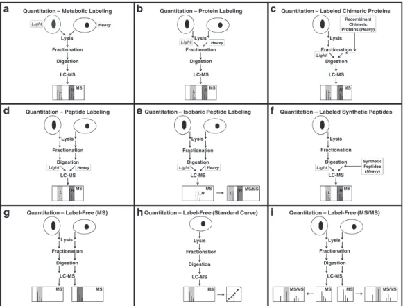
Mass spectrometry (MS)-based quantitative proteomics has been applied to solve a wide variety of biological problems, and several MS-based workflows have been developed for protein and
pep-tide quantitation (Fig. 1). In mass spectrometric quantitation
methods it is usually assumed that the measured signal has a lin-ear dependence on the amount of material in the sample for the entire range of amounts being studied. A prerequisite for accu-rate quantitation is that unwanted experimental variations in sample extraction, preparation, and analysis be minimized, and it is therefore critical that each step in the workflow is optimized for reproducibility.
One way of optimizing the reproducibility is to label the samples with stable isotopes, mix them together and perform the subsequent sample-handling steps on the mixed sample. The earlier in the workflow that the stable isotope label is introduced and the sam-ples mixed, the smaller is the effect of variations in sample handling.
1. Introduction
David Fenyö (ed.), Computational Biology,Methods in Molecular Biology, vol. 673, DOI 10.1007/978-1-60761-842-3_13, © Springer Science+Business Media, LLC 2010
Metabolic labeling (1,2) provides the earliest possible
introduc-tion of stable isotope labels into the sample (Fig. 1a). Here, labels
are introduced as isotopically distinct metabolic precursors, and the samples can be mixed before all subsequent steps in the work-flow. It is important to monitor the level of incorporation of the label, but this can, for example, be done by using two heavy labels
that are incorporated into the samples with equal efficiency (3). In
cases when metabolic labeling is not feasible, the stable isotope
labels also can be introduced later in the workflow (4–9) by heavy
isotope labeling of proteins (Fig. 1b, c) or peptides (Fig. 1d–f ).
In general, stable isotope labels need to be designed carefully in order to prevent introducing systematic errors caused by dissimi-lar behavior of the compounds with different labels. For example, it has been observed that using hydrogen/deuterium substitution in the heavy label can affect the retention time of the labeled
pep-tides, while 12C/13C substitution does not have any observable
effect on the retention time (10).
Fractionation Digestion LC-MS Lysis Quantitation – Label-Free (MS) MS MS Fractionation Digestion LC-MS Lysis MS/MS MS MS MS/MS Quantitation – Label-Free (MS/MS) L
Quantitation – Metabolic Labeling
Fractionation Digestion LC-MS Light Heavy Lysis MS H L Fractionation Digestion LC-MS
LightLysis Heavy Quantitation – Protein Labeling
MS H Fractionation Digestion LC-MS Lysis MS Light Recombinant Chimeric Proteins (Heavy) Quantitation – Labeled Chimeric Proteins
H L Fractionation Digestion LC-MS Light Heavy Lysis
Quantitation – Peptide Labeling
MS L H Fractionation Digestion LC-MS Light Lysis Synthetic Peptides (Heavy) Quantitation – Labeled Synthetic Peptides
MS H L c b a f e d i h g Fractionation Digestion LC-MS Lysis
Quantitation – Label-Free (Standard Curve)
MS Fractionation Digestion LC-MS Light Heavy Lysis MS MS/MS
Quantitation – Isobaric Peptide Labeling
L H L,H
Fig. 1. Workflows for mass spectrometry-based protein and peptide quantitation. (a) Metabolic labeling (1, 2). (b) Protein labeling (4). (c) Chimeric recombinant protein labeling (8, 9). (d) Peptide labeling (4, 5). (e) Isobaric peptide labeling (7 ). (f) Synthetic peptide labeling (6). (g) Label-free quantitation using the intensity of precursor ions (11–13). (h) Label-free quantitation using the intensity of precursor ions and a standard curve. (i) Label-free quantitation using the intensity of fragment ions.
Label-free methods (11–13) for quantitation are often used when the introduction of stable isotopes is impractical (e.g., in many animal studies) or the cost is prohibitive (e.g., in biomarker studies where a relatively large number of samples need to be analyzed). Three label-free quantitation workflows are shown in
Fig. 1g–i. In these workflows the different samples are analyzed
separately and it is therefore critical that each step of the workflow is carefully optimized for reproducibility. In label-free quantita-tion workflows, usually the peptide ion peaks are integrated and used as a measure of quantity. This allows the quantity of protein
and peptides to be compared in different samples (Fig. 1g) or the
absolute quantity can be calculated using a standard curve
(Fig. 1h). The peptide fragment ions can also be used for
quanti-tation by integrating one or more of their peaks (Fig. 1i) as, for
example, in Multiple Reaction Monitoring (MRM) (14). Using
fragment ions for quantitation provides increased specificity because in addition to requiring the mass of the precursor ion be close to its predicted mass, the masses of the fragment ions are also required to be correct. Because peptides fragment in a sequence-specific manner, additional specificity can be gained by requiring that the relative intensities of the fragment ions do not deviate from the expected intensities. Alternative methods for quantitation using fragment mass spectra do not integrate peaks but are based on the results of searching protein sequence collec-tions (see Note 1).
Currently, there are several software packages available for analysis of data from these different workflows where the quanti-tation is done by integrating peaks of ions that correspond to peptides or their fragments (see Note 2 for a few examples). Here, we describe how the mass spectra are processed to allow for find-ing the peptide peaks, detectfind-ing interference, and integratfind-ing the peaks to obtain a measure of the amount of material present in the samples.
Step 1: Detecting peptide peaks. Peptide peaks of interest for
quan-titation may range between smooth peaks with a large signal-to-noise ratio and noisy peaks that are barely above the background. The width of these peaks is, however, characteristic of the resolu-tion of the mass spectrometer, the data acquisiresolu-tion parameters
used, as well as the mass-to-charge ratio (m/z) of the peptide.
Therefore, peaks can readily be detected by scanning the mass spectra for local maxima of the expected width (see Note 3). In addition, peptides are not observed as a single peak in mass spec-trometry, but as a cluster of peaks, because of the presence of
2. Methods
small amounts of stable heavy isotopes in nature (e.g., 1.11% 13C)
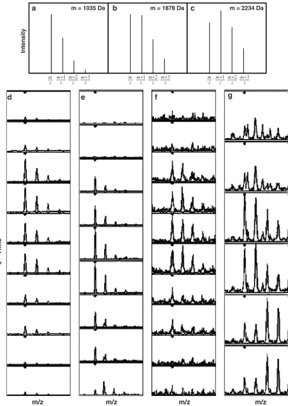
and each peptide contains many carbon atoms. The relative inten-sities of the peaks in these isotope clusters are characteristic of the atomic composition of the peptides and they are strongly
dependent on the peptide mass (Fig. 2a–c, see Note 4).
A majority of quantitation experiments are performed by coupling liquid chromatography with mass spectrometry, which introduces a retention time dimension. During these experiments, usually the same peptide is observed during several adjacent time
points (Fig. 2d–g) with highly abundant peptides typically being
observed over larger time windows than low-abundance peptides.
But even with separation in both m/z and retention time, it is not
uncommon to have unwanted interference between peaks from different peptides (Fig. 2e, g).
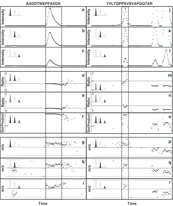
Step 2: Detecting interference. The following characteristics of
peptide peaks can be used as filters to differentiate them from interfering and non-peptide peaks: (1) the width of individual
peaks in m/z and retention time, (2) the intensity distribution of
the isotope clusters, and (3) the measured peptide m/z. These
characteristics are shown in Fig. 3 for two peptides. The width of
individual peaks as a function of m/z is highly characteristic of the instrument parameters with very little variation and therefore a narrow peak width filter can be used. The width of individual
peaks as a function of retention time (Fig. 3a–c, j–l) shows larger
variation. This variation is mainly dependent on the peak intensity and the elution time, although strong peptide sequence depen-dent variation can also be observed, and therefore a wider filter must be applied. High-accuracy measurement of peptide mass is a sensitive and selective filter that is highly reproducible even at
the tails of the peak where the intensity is low (Fig. 3g–i, p–r).
The shape of the isotope distribution is also a sensitive and selec-tive filter that can be used to detect interference from other peaks
(Fig. 3d–f, m–o). A convenient measure of the similarity of
iso-tope distributions is the dot product (see Note 5) between them
(Fig. 3f, o). The dot product can be applied to compare sets
con-taining any number of peaks, for example, to detect interferences when a set of fragment ions is monitored in a MRM experiment.
In the example shown in Fig. 3, dot product analysis of the
chro-matograms shown in the panels on the right shows that only the first isotope cluster corresponds to the peptide of sequence YVLTQPPSVSVAPGQTAR, while the second and third peaks are interfering peaks from peptides whose first three isotope peaks have a similar m/z, but their relative intensity is different.
Step 3: Measuring peptide quantity. The quantity of peptides is
measured by calculating the height or the area of the corresponding peaks in the ion chromatograms. Careful background subtraction is essential for accurate determination of both the height and the
Fig. 2. Isotope distributions of peptides. (a–c) The isotope distribution of peptides is strongly dependent on the peptide mass (see Note 4). (d–g) Examples of peptide isotope distributions observed by LC-MS with different levels of interfer-ence from other peaks acquired using quadrupole time-of-flight MS.
In te n si ty m = 1035 Da m = 1878 Da m = 2234 Da a b c z m+1 z m+2 z m+3 z m z m+1 z m+2 z m+3 z m z m+1 z m+2 z m+3 z m d e f g m/z m/z m/z m/z T im e
a b c d e In te n si ty In te n si ty In te n si ty R at io R at io D o t P ro d u ct 1 0.9 0 1 2 f j k l m n In te n si ty In te n si ty In te n si ty 1 0.9 o m /z m /z m /z Time g h i p q r m /z m /z m /z Time YVLTQPPSVSVAPGQTAR AADDTWEPFASGK 0 1 2 R at io R at io D o t P ro d u ct 0 1 2 0 1 2
Fig. 3. Examples of the variation in mass measurements and the shape of isotope distributions. (a–i) Peptide with amino acid sequence: AADDTWEPFASGK; j–r) Peptide with amino acid sequence: YVLTQPPSVSVAPGQTAR. Panels from top to
bottom: The intensity distribution of the first (a, j), second (b, k), and third (c, l) isotope peaks as a function of time; the distribution of normalized intensities of the second (d, m) and the third (e, n) isotope peaks normalized to the first isotope peak (the line represents the expected ratio based on the amino acid sequence); The normalized dot product of the three first peaks of the measured and the theoretical isotope distributions (f, o); the m/z distribution of the first (g, p), second (h, q), and third (i, r) isotope peaks as a function of time (the solid line represents the mass predicted from the amino acid sequence and the dotted lines correspond to ±5 ppm).
area of peaks (see Note 6). The advantage of using the height of the peak as the measure of quantity is the simplicity and robust-ness of its calculation (e.g., the average or median height for a few points around the centroid can be used). The peak height is a good measure of quantity if the width of the peak does not vary between samples and the signal is strong with little noise. In con-trast, the peak area is a better measurement of quantity when there is substantial noise because many more data points are used, but it is much more sensitive to interference from other peaks
because of the larger area in the m/z and retention time space
that is used. The difficulty in calculating the peak area is in
decid-ing where the peak ends and the background starts in both m/z
and retention time dimensions. This determination can be very challenging for peaks with long tails. It is also important to use the same peak limits for a specific peptide in all samples. One way of circumventing the problem of finding the peak limits is to select a function and fit its parameters (e.g., centroid, width, skewness, etc.) to the peak and integrate the function. However, often it is not straightforward to find a function that fits well to all peaks in the spectrum.
Step 4: Matching peptides from different experiments. In many
quantitation studies more than one experiment (i.e., replicates and/or multiple samples) is performed. This requires the match-ing of the peptides quantified in the different experiments. For successful matching of peptides, the retention time scales of all experiments have to be aligned, because there are always uncon-trolled variations in the experimental conditions that affect the peptide retention times in a nonlinear manner. This alignment can be done by identifying peaks present in all experiments that can be used as landmarks. These peaks are matched across experiments using either their mass and retention time, or their identity as determined by tandem MS. A smooth function is fitted to the retention times of these landmarks and used for aligning the reten-tion times of all quantified peptides. The residual difference in retention time for the landmarks can be used to estimate the uncertainty in the alignment.
For some mass spectrometers, the m/z scale needs to be
cali-brated between experiments. This mass calibration can be done using the same landmarks as used for retention time alignment. When experiments are aligned in retention time and are mass cali-brated, the quantified peptides can be matched within windows
determined by the uncertainty in the retention time and the m/z.
The measured intensities of peptide peaks commonly vary from experiment to experiment in a global manner. It is therefore advis-able to design experiments so that only a few of the quantified peptides have changes related to the hypothesis, and the majority of peptides change because of random variations in the experimen-tal conditions. The randomly changing peptides can be used to
normalize the overall intensity using either their median change in the intensity ratios or by fitting an intensity dependent smooth function to the measured intensity ratios.
Step 5: Calculating protein quantity. Protein quantity can be
estimated by measuring of peptide quantities. There are, how-ever, several factors that can make the estimates of protein quan-tity uncertain even when highly accurate peptide quantities have been obtained. Because only a few peptides are typically measured for a given protein, these peptides might not be sufficient to define all isoforms of the protein that are present in the sample – i.e., some of the peptide sequences might be shared with other proteins, making them only suitable for quantitating the group of proteins. A few peptides might also be modified, and the change in the amount of the modified and unmodified forms of the protein is often not the same. Despite these issues, a reasonable estimate of the protein quantity can often be obtained even when only a few of its peptides are quantified. When many peptides are observed for a given protein it can be possible to even calculate the variation in quantity of several isoforms.
Step 6: Determination of the significance of the change in quantity.
The significance of a measured change in quantity can be calcu-lated if the distribution of random quantity changes (due to uncontrolled variation of experimental conditions) is known
(Fig. 4a). This distribution can be obtained by analysis of
techni-cal and biologitechni-cal replicates. When the distribution of random quantity changes is known, the significance of a measured change in quantity can be calculated by integrating under the curve from the measured change in quantity to infinity and dividing this area by the area under the entire distribution of random changes. This value represents the probability that the measured quantity change was obtained from purely random variations, that is, the probabil-ity of rejecting the null hypothesis that there is no change in the experimental conditions. The distribution of random quantity changes is strongly dependent on the experimental conditions and the workflow that is chosen. For example, for label-free quan-titation the distribution of random quantity changes depends on
the number of replicates obtained (Fig. 4b–g). It is important to
design quantitation experiments to minimize the width of the distribution of random quantity changes to allow for detection of small nonrandom changes.
1. Alternative methods for quantitation search fragment mass spectra against a protein sequence collection and use the search results for quantitation. One method uses the number
3. Notes
of different fragment mass spectra that identifies a peptide as
a measure of its quantity (15). Another method calculates a
measure that is based on the fraction of the protein sequence
that the identified peptides cover (16). However, these
alter-native methods that are not based on peak integration are generally less accurate when only a few fragment spectra or peptides are observed for a given protein because of the limited statistics. On the other hand, they are less sensitive to interference and can often be more robust.
2. There are many software packages available for quantitation. A few examples of freely available software are listed below:
–1 –0.5 0 0.5 1 log2(ratio) 1-3-1 3-3-1 –1 –0.5 0 0.5 1 log2(ratio) 1-1-1 3-3-1 –1 –0.5 0 0.5 1 log2(ratio) 6-3-1 3-3-1 –1 –0.5 0 0.5 1 log2(ratio) 3-6-1 3-3-1 –1 –0.5 0 0.5 1 log2(ratio) 3-3-3 3-3-1 –1 –0.5 0 0.5 1 log2(ratio) 3-1-1 3-3-1 log2(ratio) a d c b g f e
Fig. 4. (a) The distribution that represents the null hypothesis, that is, that a given ratio is random. This distribution can be obtained by analysis of samples where only random variation is expected (technical and biological replicates). Then the significance of a ratio measurement can be calculated by integrating this distribution from the measured ratio to infinity. (b–g) Combining data from repeat analysis makes the distribution that represents the null hypothesis narrower, and smaller changes can be detected. Examples of the effect of replicate analysis on the protein ratio distribution for a workflow comprising immunoprecipitation, protein fractionation, and digestion (simulated data based on measurements of the variation in the individual steps) (26). Only limited improvements are observed beyond 3, 3, 1 repeat analyses for immunoprecipitation, protein fractionation and digestion, respectively (solid curves). Dotted curves: (b) 1, 1, 1; (c) 1, 3, 1; (d) 3, 1, 1; (e) 3, 3, 3; (f ) 3, 6, 1; (g) 6, 3, 1 repeat analyses for immunoprecipitation, protein fractionation and digestion, respectively.
Name Type Location
ASAPratio (17) ICAT
SILAC http://tools.proteomecenter.org/wiki/index.php?title=Software:ASAPRatio
MaxQuant (18, 19) SILAC http://www.maxquant.org/
MSQuant (20) SILAC http://msquant.sourceforge.net/
Pview (21) SILAC Label-free http://compbio.cs.princeton.edu/pview/
Quant (22) iTRAQ http://sourceforge.net/projects/protms/
RAAMS (23) 16O/18O http://informatics.mayo.edu/svn/trunk/
mprc/raams/index.html
Skyline (24) MRM http://proteome.gs.washington.edu/ software.html
3. For a mass spectrum where I(k) is the measured intensity at a
point k with 0 ≤k≤N, and N is the total number of points in the mass spectrum. The peaks are detected by calculating the sum, − < =
∑
| | /2 ( ) ( ) l k l wS l I k over the expected peak width wl for
each point, l, in the spectrum, and detecting local maxima in
S(l). In cases where there is sufficient noise in the spectrum
the signal-to-noise ratio is calculated by taking the ratio of the root mean square (RMS) of the intensities over the peak ( − < =
∑
− 2 | | /2 ˆ RMS ( ( ) ) / l l k l wI k I w, where Iˆ is the mean intensity
over the peak) and the RMS of the intensities in a nearby region where there are no peaks (see Note 6).
4. Peptides are observed as clusters of peaks in mass spectrometry, because of the presence of small amounts of stable heavy
iso-topes in nature (e.g., 0.015% 2H, 1.11% 13C and 0.366% 15N,
0.038% 17O, 0.200% 18O, 0.75% 33S, 4.21% 34S, 0.02% 36S). The
intensities of the isotope distribution are calculated accurately by including all possible isotopes. The largest effect comes
from 13C and a first order estimate of the relative peak
intensi-ties is given by m(1 )n m m n T p p m − = −
, where Tm is the
inten-sity of peak m in the distribution, m is the number of 13C, n
the total number of carbon atoms in the peptide, and p is the
probability for 13C (i.e., 1.11%). The isotope distribution of
peptides is strongly dependent on the peptide mass because the number of atoms increases with mass, and therefore the probability increases for having one or more of the naturally occurring heavy isotopes.
5. The normalized dot product between the measured intensities,
1 2
( , , , )I I In
= …
I and theoretical intensities T=( , , , )T T1 2 …Tn
= = = ⋅ =
∑
∑ ∑
2 2 1 1 1 / | || | n n n k k k k k k k I T I T I TI T . The range of the normalized
dot product is from −1 to 1. If the measured and theoretical intensities are identical the resulting dot product is 1 and any differences between them will result in lower values of the dot product.
6. Low-frequency background can be removed by fitting a smooth curve to the regions of the mass spectrum where there are no peaks. This smoothing can, for example, be achieved by applying a very wide and strong smoothing func-tion to the entire spectrum, which will result in a smooth function slightly higher than the background. Subsequently, points in the original spectrum that are far above this smooth curve are removed (i.e., the peaks). The smoothing proce-dure is repeated, this time without including the peaks, to produce a smooth function that will closely follow the
back-ground of the spectrum (25).
Acknowledgments
This work was supported by funding provided by the National Institutes of Health Grants RR00862, RR022220, NS050276, and CA126485, the Carl Trygger foundation, and the Swedish research council.
References
1. Y. Oda, K. Huang, F.R. Cross, D. Cowburn, and B.T. Chait (1999) Accurate quantitation of protein expression and site-specific phosphory-lation, Proc Natl Acad Sci USA, 96, 6591–6. 2. S.E. Ong, B. Blagoev, I. Kratchmarova, D.B.
Kristensen, H. Steen, A. Pandey, and M. Mann (2002) Stable isotope labeling by amino acids in cell culture, SILAC, as a simple and accurate approach to expression proteomics, Mol Cell Proteomics, 1, 376–86.
3. B. Schwanhausser, M. Gossen, G. Dittmar, and M. Selbach (2009) Global analysis of cel-lular protein translation by pulsed SILAC, Proteomics, 9, 205–9.
4. S.P. Gygi, B. Rist, S.A. Gerber, F. Turecek, M.H. Gelb, and R. Aebersold (1999) Quantitative analysis of complex protein mix-tures using isotope-coded affinity tags, Nat Biotechnol, 17, 994–9.
5. O.A. Mirgorodskaya, Y.P. Kozmin, M.I. Titov, R. Korner, C.P. Sonksen, and P. Roepstorff (2000) Quantitation of peptides and proteins
by matrix-assisted laser desorption/ionization mass spectrometry using (18)O-labeled inter-nal standards, Rapid Commun Mass Spectrom, 14, 1226–32.
6. S.A. Gerber, J. Rush, O. Stemman, M.W. Kirschner, and S.P. Gygi (2003) Absolute quantification of proteins and phosphopro-teins from cell lysates by tandem MS, Proc Natl Acad Sci USA, 100, 6940–5.
7. P.L. Ross, Y.N. Huang, J.N. Marchese, B. Williamson, K. Parker, S. Hattan, N. Khainovski, S. Pillai, S. Dey, S. Daniels, S. Purkayastha, P. Juhasz, S. Martin, M. Bartlet-Jones, F. He, A. Jacobson, and D.J. Pappin (2004) Multiplexed protein quantitation in Saccharomyces cerevisiae using amine-reactive isobaric tagging reagents, Mol Cell Proteomics, 3, 1154–69.
8. R.J. Beynon, M.K. Doherty, J.M. Pratt, and S.J. Gaskell (2005) Multiplexed absolute quantification in proteomics using artificial QCAT proteins of concatenated signature peptides, Nat Methods, 2, 587–9.
9. L. Anderson and C.L. Hunter (2006) Quantitative mass spectrometric multiple reaction monitoring assays for major plasma proteins, Mol Cell Proteomics, 5, 573–88. 10. E.C. Yi, X.J. Li, K. Cooke, H. Lee, B. Raught,
A. Page, V. Aneliunas, P. Hieter, D.R. Goodlett, and R. Aebersold (2005) Increased quantitative proteome coverage with (13)C/ (12)C-based, acid-cleavable isotope-coded affinity tag reagent and modified data acquisi-tion scheme, Proteomics, 5, 380–7.
11. P. Schulz-Knappe, H.D. Zucht, G. Heine, M. Jurgens, R. Hess, and M. Schrader (2001) Peptidomics: the comprehensive analysis of peptides in complex biological mixtures, Comb Chem High Throughput Screen, 4, 207–17. 12. W. Wang, H. Zhou, H. Lin, S. Roy, T.A.
Shaler, L.R. Hill, S. Norton, P. Kumar, M. Anderle, and C.H. Becker (2003) Quan-tification of proteins and metabolites by mass spectrometry without isotopic labeling or spiked standards, Anal Chem, 75, 4818–26. 13. M.C. Wiener, J.R. Sachs, E.G. Deyanova, and
N.A. Yates (2004) Differential mass spec-trometry: a label-free LC-MS method for finding significant differences in complex pep-tide and protein mixtures, Anal Chem, 76, 6085–96.
14. T.A. Addona, S.E. Abbatiello, B. Schilling, S.J. Skates, D.R. Mani, D.M. Bunk, C.H. Spiegelman, L.J. Zimmerman, A.J. Ham, H. Keshishian, S.C. Hall, S. Allen, R.K. Blackman, C.H. Borchers, C. Buck, H.L. Cardasis, M.P. Cusack, N.G. Dodder, B.W. Gibson, J.M. Held, T. Hiltke, A. Jackson, E.B. Johansen, C.R. Kinsinger, J. Li, M. Mesri, T.A. Neubert, R.K. Niles, T.C. Pulsipher, D. Ransohoff, H. Rodriguez, P.A. Rudnick, D. Smith, D.L. Tabb, T.J. Tegeler, A.M. Variyath, L.J. Vega-Montoto, A. Wahlander, S. Waldemarson, M. Wang, J.R. Whiteaker, L. Zhao, N.L. Anderson, S.J. Fisher, D.C. Liebler, A.G. Paulovich, F.E. Regnier, P. Tempst, and S.A. Carr (2009) Multi-site assessment of the precision and reproducibility of multiple reaction monitoring-based measurements of proteins in plasma, Nat Biotechnol, 27, 633–41. 15. H. Liu, R.G. Sadygov, and J.R. Yates, 3rd
(2004) A model for random sampling and esti-mation of relative protein abundance in shot-gun proteomics, Anal Chem, 76, 4193–201. 16. Y. Ishihama, Y. Oda, T. Tabata, T. Sato, T.
Nagasu, J. Rappsilber, and M. Mann (2005) Exponentially modified protein abundance index (emPAI) for estimation of absolute pro-tein amount in proteomics by the number of
sequenced peptides per protein, Mol Cell Proteomics, 4, 1265–72.
17. X.J. Li, H. Zhang, J.A. Ranish, and R. Aebersold (2003) Automated statistical analy-sis of protein abundance ratios from data gen-erated by stable-isotope dilution and tandem mass spectrometry, Anal Chem, 75, 6648–57. 18. J. Cox and M. Mann (2008) MaxQuant
enables high peptide identification rates, indi-vidualized p.p.b.-range mass accuracies and proteome-wide protein quantification, Nat Biotechnol, 26, 1367–72.
19. J. Cox, I. Matic, M. Hilger, N. Nagaraj, M. Selbach, J.V. Olsen, and M. Mann (2009) A practical guide to the MaxQuant computa-tional platform for SILAC-based quantitative proteomics, Nat Protoc, 4, 698–705.
20. P. Mortensen, J.W. Gouw, J.V. Olsen, S.E. Ong, K.T. Rigbolt, J. Bunkenborg, J. Cox, L.J. Foster, A.J. Heck, B. Blagoev, J.S. Andersen, and M. Mann (2010) MSQuant, an open source platform for mass spectrome-try-based quantitative proteomics, J Proteome Res, 9(1):393–403.
21. Z. Khan, J.S. Bloom, B.A. Garcia, M. Singh, and L. Kruglyak (2009) Protein quantification across hundreds of experimental conditions, Proc Natl Acad Sci USA, 106, 15544–8. 22. A.M. Boehm, S. Putz, D. Altenhofer, A.
Sickmann, and M. Falk (2007) Precise protein quantification based on peptide quantification using iTRAQ, BMC Bioinformatics, 8, 214. 23. C.J. Mason, T.M. Therneau, J.E.
Eckel-Passow, K.L. Johnson, A.L. Oberg, J.E. Olson, K.S. Nair, D.C. Muddiman, and H.R. Bergen, 3rd (2007) A method for automatically inter-preting mass spectra of 18O-labeled isotopic clusters, Mol Cell Proteomics, 6, 305–18. 24. B. MacLean, D.M. Tomazela, N. Shulman, M.
Chambers, G. Finney, B. Frewen, R. Kern, D.L. Tabb, D.C. Liebler and M.J. Maccoss (2010) Skyline: an open source document editor for creating and analyzing targeted proteomics experiments, Bioinformatics, 26, 966–8. 25. E.M. Woo, D. Fenyo, B.H. Kwok, H.
Funabiki, and B.T. Chait (2008) Efficient identification of phosphorylation by mass spectrometric phosphopeptide fingerprinting, Anal Chem, 80, 2419–25.
26. G. Zhang, D. Fenyo, and T.A. Neubert (2009) Evaluation of the variation in sample preparation for comparative proteomics using stable isotope labeling by amino acids in cell culture, J Proteome Res, 8, 1285–92.