Washington University in St. Louis
Washington University Open Scholarship
Engineering and Applied Science Theses &Dissertations McKelvey School of Engineering
Spring 5-15-2016
A General Framework of Large-Scale Convex
Optimization Using Jensen Surrogates and
Acceleration Techniques
Soysal Degirmenci
Washington University in St. Louis
Follow this and additional works at:https://openscholarship.wustl.edu/eng_etds
Part of theApplied Mathematics Commons, and theElectrical and Electronics Commons
This Dissertation is brought to you for free and open access by the McKelvey School of Engineering at Washington University Open Scholarship. It has been accepted for inclusion in Engineering and Applied Science Theses & Dissertations by an authorized administrator of Washington University Open Scholarship. For more information, please [email protected].
Recommended Citation
Degirmenci, Soysal, "A General Framework of Large-Scale Convex Optimization Using Jensen Surrogates and Acceleration Techniques" (2016).Engineering and Applied Science Theses & Dissertations. 157.
WASHINGTON UNIVERSITY IN ST. LOUIS School of Engineering & Applied Science Department of Electrical & Systems Engineering
Dissertation Examination Committee: Joseph A. O’Sullivan, Chair
Mark Anastasio Jr-Shin Li Arye Nehorai David G. Politte
A General Framework of Large-Scale Convex Optimization Using Jensen Surrogates and Acceleration Techniques
by
Soysal Degirmenci
A dissertation presented to the Graduate School of Arts and Sciences
of Washington University in partial fulfillment of the requirements for the degree
of Doctor of Philosophy
May 2016 St. Louis, Missouri
Contents
List of Figures . . . v
List of Tables . . . xii
List of Algorithms . . . xvii
List of Abbreviations . . . xvii
Acknowledgments . . . .xviii Abstract . . . xxi 1 Introduction . . . 1 1.1 Motivation . . . 1 1.2 Contributions . . . 4 1.3 Outline . . . 6
2 Notation and Definitions . . . 7
3 Convex Optimization Methods . . . 14
3.1 First-Order Convex Optimization Methods . . . 14
3.1.1 Gradient Descent Method . . . 15
3.1.2 Mirror Descent Method . . . 17
3.1.3 Weighted Gradient Descent Method . . . 18
3.2 Second-Order Convex Optimization Methods . . . 18
3.3 Splitting Methods . . . 20
4 Convex Optimization Using Jensen Surrogates . . . 23
4.1 Discussion on the Choice of Auxiliary Variables . . . 27
5 Convergence Analysis of Convex Optimization Using Jensen Surrogates 29 5.1 Exact Surrogate Minimization, Fixed Lg . . . 36
5.2 Inexact Surrogate Minimization, Fixed Lg . . . 41
5.3 Exact Surrogate Minimization, Changing Lg . . . 43
5.3.1 General Case . . . 43
5.3.2 Special Case: Jensen Surrogates for Poisson Log-likelihood PET . . . 44
5.4 Inexact Surrogate Minimization, Changing Lg . . . 51
6 Acceleration Methods for Convex Optimization . . . 53
6.2 Domain Based Acceleration Methods . . . 58
6.3 Momentum and Variable Step Size Based Acceleration Methods . . . 61
7 Acceleration Methods for Convex Optimization Using Jensen Surrogates 64 7.1 Range Based Acceleration Methods with Jensen Surrogates . . . 64
7.2 Domain Based Acceleration Methods with Jensen Surrogates . . . 68
7.3 Momentum and Variable Step Size Based Acceleration Methods with Jensen Surrogates . . . 71
7.4 Acceleration Using Adaptive Jensen Surrogates . . . 72
8 Applications and Results . . . 75
8.1 X-Ray Transmission Tomography . . . 75
8.1.1 Acceleration Methods . . . 81
8.1.2 Results . . . 90
8.2 Sparse Linear Regression . . . 129
8.2.1 Acceleration Methods . . . 132
8.2.2 Results . . . 134
8.3 Positron Emission Tomography, Poisson Log-likelihood . . . 155 8.3.1 Acceleration Methods . . . 157 8.3.2 Results . . . 162 8.4 Logistic Regression . . . 174 8.4.1 Acceleration Methods . . . 179 8.4.2 Results . . . 184
8.5 Sparse Logistic Regression . . . 191
8.5.1 Acceleration Methods . . . 202
8.5.2 Results . . . 204
8.6 Automatic Relevance Determination for X-Ray Transmission Tomography . . . 208 8.6.1 Algorithm . . . 212 8.6.2 Convergence Analysis . . . 215 8.6.3 Acceleration Methods . . . 223 8.6.4 Results . . . 225 9 Conclusion . . . 231 Bibliography . . . 233
Appendix A Trust Region Method for Regularized X-Ray Transmission Tomography Using Jensen Surrogates. . . 241
Appendix B Modified Trust Region Method for Regularized X-Ray Trans-mission Tomography Using Jensen Surrogates . . . 245
List of Figures
8.1 Images reconstructed with AM for two different iteration numbers. . . 92
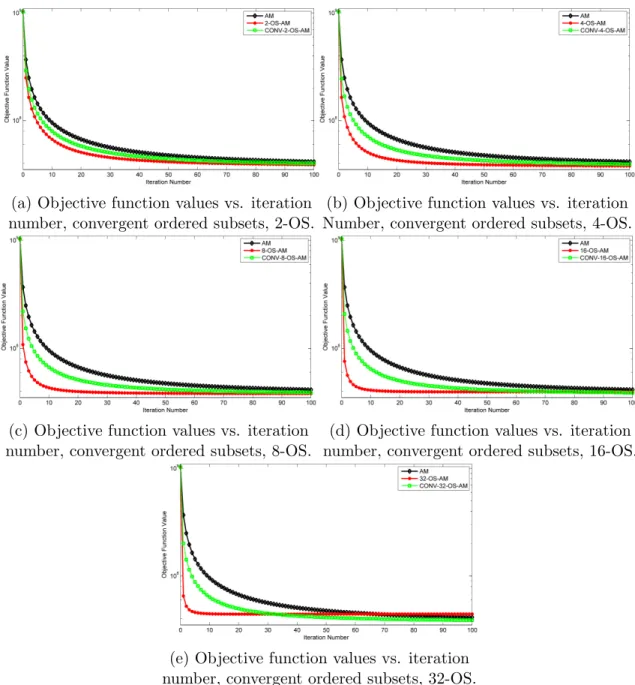
8.2 Objective function values vs. iteration number for CONV-OS-AM for different subset choices. . . 93
8.3 Images reconstructed with CONV-OS-AM for different subset choices. . . 94
8.4 Images reconstructed with OS-AM for different subset choices. . . 95
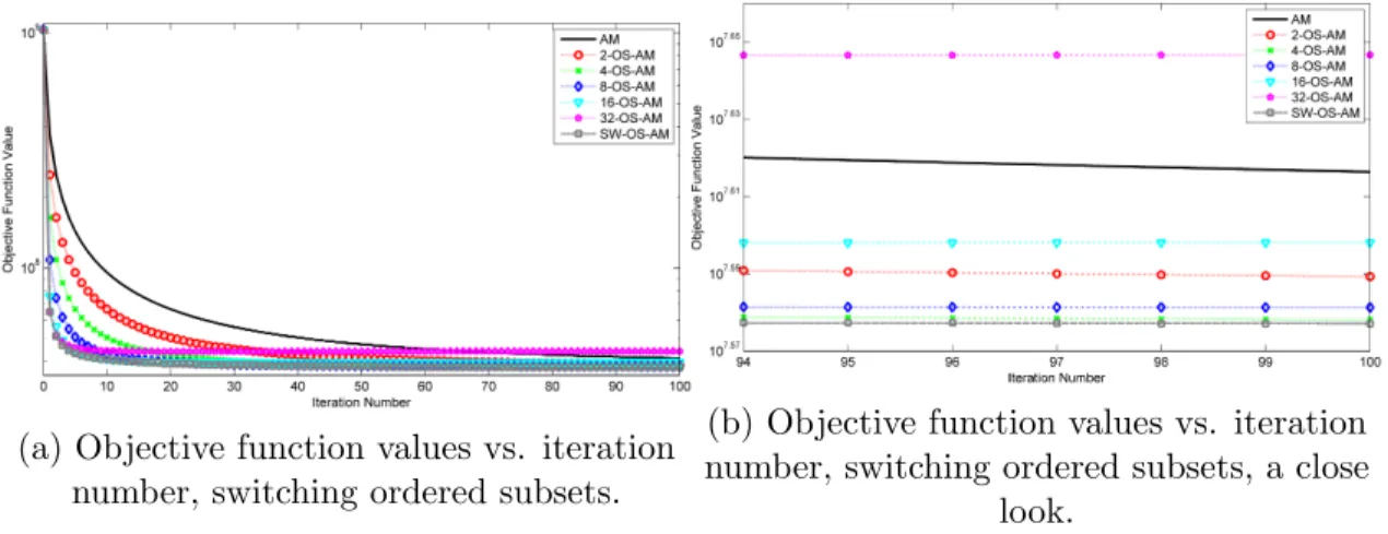
8.5 Objective function values vs. iteration number, switching ordered subsets. . 96
8.6 Objective function values vs. iteration number, different variable step size schemes. . . 96
8.7 Images reconstructed with VS-AM for different schemes. . . 97
8.8 Fan-beam geometry used for simulated experiments. . . 99
8.9 Shepp-Logan Phantom used. Image is in [0,1] color scale. . . 100
8.10 Region of interest used. . . 101
8.11 Images reconstructed from Poisson data using JSXR and GDXR at iterations 100, 1000, 5000,λ = 0, δ= 0.001. Images are in [0,1] color scale. . . 104
8.12 Images reconstructed from Poisson data using AJSXR and FJSXR at itera-tions 100, 1000, 5000, λ= 0, δ= 0.001. Images are in [0,1] color scale. . . . 105
8.13 Images reconstructed from Poisson data using AFJSXR and FGDXR at iter-ations 100, 1000, 5000,λ = 0, δ= 0.001. Images are in [0,1] color scale. . . . 106
8.14 Images reconstructed from Poisson data using JSXR and GDXR at iterations 100, 1000, 5000,λ = 1e2, δ= 0.001. Images are in [0,1] color scale. . . 107
8.15 Images reconstructed from Poisson data using AJSXR and FJSXR at itera-tions 100, 1000, 5000, λ= 1e2, δ= 0.001. Images are in [0,1] color scale. . . 108
8.16 Images reconstructed from Poisson data using AFJSXR and FGDXR at iter-ations 100, 1000, 5000,λ = 1e2, δ= 0.001. Images are in [0,1] color scale. . . 109
8.17 Images reconstructed from Poisson data using JSXR and GDXR at iterations 100, 1000, 5000,λ = 10e2, δ= 0.001. Images are in [0,1] color scale. . . 110
8.18 Images reconstructed from Poisson data using AJSXR and FJSXR at itera-tions 100, 1000, 5000, λ= 10e2, δ= 0.001. Images are in [0,1] color scale. . . 111
8.19 Images reconstructed from Poisson data using AFJSXR and FGDXR at it-erations 100, 1000, 5000, λ = 10e2, δ = 0.001. Images are in [0,1] color scale. . . 112
8.20 Images reconstructed from Poisson data using JSXR and GDXR at iterations 100, 1000, 5000,λ = 100e2,δ = 0.001. Images are in [0,1] color scale. . . 113
8.21 Images reconstructed from Poisson data using AJSXR and FJSXR at itera-tions 100, 1000, 5000, λ= 100e2,δ = 0.001. Images are in [0,1] color scale. . 114
8.22 Images reconstructed from Poisson data using AFJSXR and FGDXR at it-erations 100, 1000, 5000, λ = 100e2, δ = 0.001. Images are in [0,1] color scale. . . 115
8.23 Images reconstructed from Poisson data using JSXR and GDXR at iterations 100, 1000, 5000,λ = 1000e2,δ = 0.001. Images are in [0,1] color scale. . . . 116 8.24 Images reconstructed from Poisson data using AJSXR and FJSXR at
iter-ations 100, 1000, 5000, λ = 1000e2, δ = 0.001. Images are in [0,1] color scale. . . 117 8.25 Images reconstructed from Poisson data using AFJSXR and FGDXR at
it-erations 100, 1000, 5000, λ = 1000e2, δ = 0.001. Images are in [0,1] color scale. . . 118 8.26 Normalized function error values vs. iteration index for different algorithm
variants after 2000 iterations. . . 119 8.27 Normalized function error vs. number of full data passes for Jensen surrogate
variants and gradient descent variants for X-Ray Transmission Tomography using different λ values, 2 batches. . . 122 8.28 Normalized function error vs. number of full data passes for Jensen surrogate
variants and gradient descent variants for X-Ray Transmission Tomography using different λ values, 4 batches. . . 123 8.29 Normalized function error vs. number of full data passes for Jensen surrogate
variants and gradient descent variants for X-Ray Transmission Tomography using different λ values, 8 batches. . . 124 8.30 Normalized function error vs. number of full data passes for Jensen surrogate
variants and gradient descent variants for X-Ray Transmission Tomography using different λ values, 16 batches. . . 125 8.31 Normalized function error vs. number of full data passes for Jensen surrogate
variants and gradient descent variants for X-Ray Transmission Tomography using different λ values, 32 batches. . . 126 8.32 Normalized function error vs. number of full data passes for Jensen surrogate
variants and gradient descent variants for X-Ray Transmission Tomography using different λ values, 64 batches. . . 127 8.33 Normalized function error vs. number of full data passes for Jensen surrogate
variants and gradient descent variants for X-Ray Transmission Tomography using different λ values, 128 batches. . . 128 8.34 Normalized function value errors vs. iteration number for 3 different auxiliary
choices for JSISTA, 4 different cases of distribution ofH. . . 137 8.35 Normalized function value errors vs. iteration number for 2 different auxiliary
choices for AJSISTA, 2 different cases of the normal distribution, and different periods of auxiliary variable updates. k1 = 2.8,k2 = 0.65, k3 = 0.1 . . . 140
8.36 Normalized function value errors vs. iteration number for 2 different auxiliary choices for AJSISTA, 2 different cases of the uniform distribution, and different periods of auxiliary variable updates. k1 = 2.8,k2 = 0.65, k3 = 0.1 . . . 141
8.37 Normalized function value errors vs. iteration number for different variants of Jensen Surrogate Optimization. In parts a and c, for AJSISTA, k1 = 1,
k2 = 0.4, k3 = 0.5, TAJ S = 100 was used; for AFJSISTA, k1 = 2, k2 = 0.1,
k3 = 0.5, TAJ S = 100 was used. In parts b and d, for AJSISTA, k1 = 0.5,
k2 = 0.1, k3 = 0.5, TAJ S = 100 was used; for AFJSISTA, k1 = 1, k2 = 0.5,
8.38 Normalized function value errors vs. iteration number for Jensen surrogates variants and gradient descent variants. In parts a and c, for AJSISTA,k1 = 1,
k2 = 0.4, k3 = 0.5, TAJ S = 100 was used; for AFJSISTA, k1 = 2, k2 = 0.1,
k3 = 0.5, TAJ S = 100 was used. In parts b and d, for AJSISTA, k1 = 0.5,
k2 = 0.1, k3 = 0.5, TAJ S = 100 was used; for AFJSISTA, k1 = 1, k2 = 0.5,
k3 = 0.5,TAJ S = 100 was used. . . 143
8.39 Gaussian blurring filter used. . . 146 8.40 Original image (a) and blurred and noise added (b) cameraman images. . . . 147 8.41 Image comparison for Cameraman Image Case for several iterations, ISTA vs.
JSISTA, λ= 1e−5. . . 148 8.42 Image comparison for the Cameraman Image Case for several iterations, FISTA
vs. FJSISTA, λ= 1e−5. . . 149 8.43 Normalized function value errors vs. iteration number for the Cameraman
case, 5 different algorithms,λ = 1e−5. . . 150 8.44 Original image (a) and blurred and noise added (b) Hansen’s test image. . . 151 8.45 Image comparison for Hansen’s Test Image Case for several iterations, ISTA
vs. JSISTA, λ= 5e−4. . . 152 8.46 Image comparison for Hansen’s Test Image Case for several iterations, FISTA
vs. FJSISTA, λ= 5e−4. . . 153 8.47 Normalized function value errors vs. iteration number for Hansen’s test image
case, 5 different algorithms,λ = 5e−4. . . 154 8.48 Normalized function value errors vs. iteration number for 4 different
distribu-tion choices for JSET and FJSET. . . 163 8.49 Original Hoffman phantom used in experiments. Image is in [0,1600] color
scale. . . 165 8.50 Region of interest used in experiments. . . 167 8.51 Final images reconstructed from noiseless data using JSET and FJSET after
5000 iterations, λ= 0. Images are in [0,1600] color scale. . . 167 8.52 Images reconstructed from noisy Poisson data using JSET and FJSET at
iterations 100, 1000, 5000, λ= 0, δ= 10. Images are in [0,1600] color scale. . 168 8.53 Images reconstructed from noisy Poisson data using JSET and FJSET at
iterations 100, 1000, 5000, λ = 1e−5, δ = 10. Images are in [0,1600] color scale. . . 169 8.54 Images reconstructed from noisy Poisson data using JSET and FJSET at
iterations 100, 1000, 5000, λ = 1e−4, δ = 10. Images are in [0,1600] color scale. . . 170 8.55 Images reconstructed from noisy Poisson data using JSET and FJSET at
iterations 100, 1000, 5000, λ = 1e−3, δ = 10. Images are in [0,1600] color scale. . . 171 8.56 Normalized function error vs. iteration index for JSET and FJSET algorithms.172 8.57 Normalized function error vs. number of full data passes full and stochastic
methods proposed for Emission Tomography for different number of batches,
λ= 0. . . 173 8.58 Zero-one loss function and logistic regression loss function vs. prediction l
8.59 Normalized function error vs. iteration index for Jensen surrogate variants and gradient descent variants for Logistic Regression using differentλ values. 187 8.60 Validation error vs. iteration index for Jensen surrogate variants and gradient
descent variants for Logistic Regression using differentλ values. . . 188 8.61 Normalized function error vs. number of full data passes for Jensen surrogate
variants and gradient descent variants for Logistic Regression using different
λ values, 2 batches. . . 192 8.62 Normalized function error vs. number of full data passes for Jensen surrogate
variants and gradient descent variants for Logistic Regression using different
λ values, 4 batches. . . 193 8.63 Normalized function error vs. number of full data passes for Jensen surrogate
variants and gradient descent variants for Logistic Regression using different
λ values, 8 batches. . . 194 8.64 Normalized function error vs. number of full data passes for Jensen surrogate
variants and gradient descent variants for Logistic Regression using different
λ values, 16 batches. . . 195 8.65 Normalized function error vs. number of full data passes for Jensen surrogate
variants and gradient descent variants for Logistic Regression using different
λ values, 32 batches. . . 196 8.66 Normalized function error vs. number of full data passes for Jensen surrogate
variants and gradient descent variants for Logistic Regression using different
λ values, 64 batches. . . 197 8.67 Normalized function error vs. number of full data passes for Jensen surrogate
variants and gradient descent variants for Logistic Regression using different
λ values, 128 batches. . . 198 8.68 Normalized function error vs. iteration index for Jensen surrogate variants
and gradient descent variants for Sparse Logistic Regression using differentλ
values. . . 206 8.69 Validation error vs. iteration index for Jensen surrogate variants and gradient
descent variants for Sparse Logistic Regression using different λ values. . . . 207 8.70 Fan-beam geometry used for simulated experiments. . . 226 8.71 Shepp-Logan phantom used to generate simulated data in experiments. . . . 227 8.72 Final mean and variance images for different variants of the ARD Algorithm
after 100 iterations. Mean images are shown in color scale [0,1] whereas variance images are shown in [7.5e−6,1e−5]. . . 228 8.73 Normalized Objective Function Errors, (F(z(n))−F(z(∗)))/F(z(∗)) for
List of Tables
2.1 Table for notation used. . . 8 8.1 Different auxiliary variable choices for Least-Squares Jensen Surrogates convex
optimization and the resultant step sizes. . . 131 8.2 Final accuracy percentage on validation set after 5000 iterations for different
λ values and algorithms. . . 186 8.3 Lipschitz gradient constants computed for different number of batch settings
using Cover-type dataset. . . 189 8.4 Final accuracy percentage on validation set after 5000 iterations for different
List of Algorithms
1 A generic iterative algorithm . . . 11
2 Generic Convex Optimization Algorithm Using Jensen Surrogates . . . 27
3 Generic Convex Optimization Algorithm Using Jensen Surrogates, Inexact Jensen Surrogate Minimization . . . 42
4 Generic Incremental Convex Optimization Algorithm . . . 56
5 Generic Random Block Coordinate Descent Method (BCD) . . . 60
6 Cyclic Convex Optimization Using Jensen Surrogates . . . 65
7 Stochastic Convex Optimization Using Jensen Surrogates . . . 65
8 Stochastic Incremental Convex Optimization Using Jensen Surrogates . . . . 67
9 Stochastic Averaging Convex Optimization Using Jensen Surrogates . . . 68
10 Randomized Block Coordinate Convex Optimization Using Jensen Surrogates 70 11 Fast Convex Optimization Using Jensen Surrogates . . . 71
12 Convex Optimization Using Adaptive Jensen Surrogates . . . 74
13 Regularized Poisson Log-likelihood X-Ray Transmission Tomography Opti-mization Using Jensen Surrogates (JSXR) . . . 79
14 Regularized Poisson Log-likelihood X-Ray Transmission Tomography Opti-mization Using Jensen Surrogates, Simplified . . . 80
15 Ordered Subsets Algorithm using Jensen Surrogates for X-Ray Transmission Tomography (OS-JSXR) . . . 82
16 Convergent Ordered Subsets Algorithm using Jensen Surrogates for X-Ray Transmission Tomography (CONV-OS-JSXR) . . . 82
17 Switching Ordered Subsets Algorithm using Jensen Surrogates for X-Ray Transmission Tomography (SW-OS-JSXR) . . . 83
18 Stochastic Jensen Surrogates Optimization for X-Ray Transmission Tomog-raphy (SJSXR) . . . 84
19 Stochastic Incremental Jensen Surrogates Optimization for X-Ray Transmis-sion Tomography (SIJSXR) . . . 84
20 Stochastic Averaging Jensen Surrogates Optimization for X-Ray Transmission Tomography (SAJSXR) . . . 85
21 Variable Step Size Algorithm using Jensen Surrogates for X-Ray Transmission Tomography (VSS-JSXR) . . . 85
22 Fast Optimization using Jensen Surrogates for X-Ray Transmission Tomog-raphy (FJSXR) . . . 88
23 Accelerated Optimization using Adaptive Jensen Surrogates for X-Ray Trans-mission Tomography (AJSXR) . . . 89
24 Fast Optimization using Adaptive Jensen Surrogates for X-Ray Transmission Tomography (AFJSXR) . . . 90 25 Gradient Descent Algorithm for X-Ray Transmission Tomography (GDXR) . 102 26 Fast Gradient Descent for X-Ray Transmission Tomography (FGDXR) . . . 103 27 Stochastic Gradient Descent Algorithm for X-Ray Transmission Tomography
(SGDXR) . . . 120 28 Stochastic Incremental Gradient Descent for X-Ray Transmission
Tomogra-phy (SIGDXR) . . . 121 29 Stochastic Averaging Gradient Descent Algorithm for X-Ray Transmission
Tomography (SAGDXR) . . . 121 30 Least Squares Minimization using Jensen Surrogates . . . 130 31 Iterative Shrinkage Thresholding Algorithm (ISTA) . . . 132 32 Jensen Surrogates Iterative Shrinkage Thresholding Algorithm (JSISTA) . . 132 33 Fast Iterative Soft Thresholding Algorithm (FISTA) [6] . . . 133 34 Fast Jensen Surrogate Iterative Soft Thresholding Algorithm (FJSISTA) . . 133 35 Adaptive Jensen Surrogates Iterative Shrinkage Thresholding Algorithm
(AJ-SISTA) . . . 134 36 Adaptive Fast Jensen Surrogate Iterative Soft Thresholding Algorithm
(AFJ-SISTA) . . . 135 37 Jensen Surrogates Optimization for Maximum Likelihood Estimation for
Emis-sion Tomography (JSMLET) . . . 156 38 Jensen Surrogates Optimization for Penalized Likelihood Estimation for
Emis-sion Tomography (JSET) . . . 157 39 Stochastic Jensen Surrogates Optimization for Penalized Likelihood
Estima-tion for Emission Tomography (SJSET) . . . 159 40 Stochastic Incremental Jensen Surrogates Optimization for Penalized
Likeli-hood Estimation for Emission Tomography (SIJSET) . . . 159 41 Stochastic Averaging Jensen Surrogates Optimization for Penalized
Likeli-hood Estimation for Emission Tomography (SAJSET) . . . 159 42 Fast Jensen Surrogates Optimization for Penalized Likelihood Estimation for
Emission Tomography (FJSET) . . . 160 43 Adaptive Jensen Surrogates Optimization for Maximum Likelihood
Estima-tion for Emission Tomography (AJSET) . . . 161 44 Jensen Surrogates Optimization for Regularized Logistic Regression (JSLR) . 178 45 Stochastic Jensen Surrogates Optimization for Regularized Logistic
Regres-sion (SJSLR) . . . 179 46 Stochastic Incremental Jensen Surrogates Optimization for Regularized
Lo-gistic Regression (SIJSLR) . . . 180 47 Stochastic Incremental Jensen Surrogates Optimization for Regularized
Lo-gistic Regression (SIJSLR) . . . 180 48 Fast Jensen Surrogates for Regularized Logistic Regression (FJSLR) . . . 181 49 Adaptive Jensen Surrogates Optimization for Regularized Logistic Regression
(AJSLR) . . . 182 50 Adaptive Fast Jensen Surrogates Optimization for Regularized Logistic
51 Gradient Descent Algorithm for Logistic Regression (GDLR) . . . 185 52 Fast Gradient Descent Algorithm for Logistic Regression (FGDLR) . . . 185 53 Stochastic Gradient Descent Algorithm for Logistic Regression (SGDLR) . . 190 54 Stochastic Incremental Gradient Descent Algorithm for Logistic Regression
(SIGDLR) . . . 190 55 Stochastic Averaging Gradient Descent Algorithm for Logistic Regression
(SAGDLR) . . . 190 56 Jensen Surrogates Optimization for Sparse Logistic Regression (JSSLR) . . . 201 57 Fast Jensen Surrogates Optimization for Sparse Logistic Regression (FJSSLR) 202 58 Adaptive Jensen Surrogates for Sparse Logistic Regression (AJSSLR) . . . . 203 59 Adaptive Fast Jensen Surrogates Optimization for Sparse Logistic Regression
(AFJSSLR) . . . 203 60 Gradient Descent Algorithm for Sparse Logistic Regression (GDSLR) . . . . 204 61 Fast Gradient Descent Algorithm for Sparse Logistic Regression (FGDSLR) . 204 62 Automatic Relevance Determination (ARD) Algorithm Using Jensen
Surro-gates for Transmission Tomography . . . 215 63 Modified Automatic Relevance Determination (ARD) Algorithm Using Jensen
Surrogates for Transmission Tomography . . . 223 64 Fast Automatic Relevance Determination (FARD) Algorithm Using Jensen
Surrogates for Transmission Tomography . . . 224 65 Automatic Relevance Determination Algorithm Using Adaptive Jensen
Sur-rogates for Transmission Tomography (AARD) . . . 225 66 Trust Region Newton’s Method for the Image Update Part in X-Ray
Trans-mission Tomography Algorithm with Jensen Surrogates . . . 244 67 Modified Trust Region Newton’s Method for the Image Update Part in X-Ray
Acknowledgments
I would like to thank my mother, Zehra, and my father, Refik, for everything. I am fortunate to have had their continuous love and support throughout my life. Their physical and emotional labors have allowed me the opportunity to pursue my goals, and for that I am eternally grateful. Moreover, I thank my mother for the optimism and guidance she has been channeling from thousands of miles away. For years she has offered her patience, love, and insight, and this has been invaluable as I conduct my PhD research and write my dissertation. I would like to thank my aunt, Zeliha, my uncle, Ali, and my cousin, Melis, for the support they offer and the happiness they bring to my life. I would also like to thank my grandparents, Bedriye and Nuri; their wisdom and counsel has not been lost on me. Though they are gone, their memories bring me great happiness and comfort.
I am grateful to my girlfriend, Paige, whose cheerfulness has helped me keep my head in times of stress, and whose confidence in me has never waned. I am full of appreciation for her family, who have treated me like one of their own, and whom I surely count among mine; their warmness and generosity has made St. Louis feel like home.
A special thanks goes to the educators I have had the pleasure of learning from during my undergraduate and high school tenure. Good advancements require good foundations, and I was lucky enough to have such foundations thanks to them. I am also thankful for my friends in Turkey, who encourage and motivate me, and have offered their goodwill time and time again. Their presence, even remotely, has made my life better.
I thank many graduate students, distinguished faculty, and engineers who have been helpful during my studies. These include, but are not limited to, Carl M. Bosch, Nawfel Tricha, Assaf
Mesika, Dr. Yan Kaganovsky, Sean Corrigan, Michael Hollenbeck, Jason Barlow, Terence Bordelon, Dr. Ikenna Odinaka, Dr. Qiaofeng Xu, Dr. Yaqi Chen, Jingwei Lu, Daheng Li, Dr. Lawrance Carlin, Dr. David J. Brady, Shaobo Han, Ke Li, and Homayoon Ranjbar.
I thank my advisor Dr. David G. Politte, for his continuous support and assistance during my research. I have learned a lot from him about research methodology and am grateful that he has always been keen in his consideration of the various thoughts and ideas I have brought to him.
I thank the members of my committee for their time and invaluable comments and critique of this work: Prof. Joseph A. O’Sullivan, Dr. David G. Politte, Prof. Arye Nehorai, Prof. Mark Anastasio, and Dr. Jr-Shin Li.
Finally, I would like to thank my advisor Prof. Joseph A. O’Sullivan for giving me this opportunity. His guidance has taught me how to conduct research and pursue a career. Our fruitful discussions, his availability, and his readiness to help, listen, and offer guidance have been instrumental in the production of this work.
This work was supported under contracts HSHQDC-14-C-B0011 to SureScan Corporation, by the United States Department of Homeland Security Science and Technology Directorate, and HSHQDC-11-C-0083 by the United States Department of Homeland Security Science and Technology Directorate, Explosives Division.
Soysal Degirmenci
Washington University in Saint Louis May 2016
ABSTRACT OF THE DISSERTATION
A General Framework of Large-Scale Convex Optimization Using Jensen Surrogates and Acceleration Techniques
by
Soysal Degirmenci
Doctor of Philosophy in Electrical Engineering Washington University in St. Louis, 2016
Professor Joseph A. O’Sullivan, Chair
In a world where data rates are growing faster than computing power, algorithmic accelera-tion based on developments in mathematical optimizaaccelera-tion plays a crucial role in narrowing the gap between the two. As the scale of optimization problems in many fields is getting larger, we need faster optimization methods that not only work well in theory, but also work well in practice by exploiting underlying state-of-the-art computing technology.
In this document, we introduce a unified framework of large-scale convex optimization using Jensen surrogates, an iterative optimization method that has been used in different fields since the 1970s. After this general treatment, we present non-asymptotic convergence anal-ysis of this family of methods and the motivation behind developing accelerated variants. Moreover, we discuss widely used acceleration techniques for convex optimization and then investigate acceleration techniques that can be used within the Jensen surrogate framework while proposing several novel acceleration methods. Furthermore, we show that proposed methods perform competitively with or better than state-of-the-art algorithms for several
applications including Sparse Linear Regression (Image Deblurring), Positron Emission To-mography, X-Ray Transmission ToTo-mography, Logistic Regression, Sparse Logistic Regression and Automatic Relevance Determination for X-Ray Transmission Tomography.
Chapter 1
Introduction
1.1
Motivation
Optimization has been prevalent everywhere for centuries, formally or informally, in differ-ent fields, and for differdiffer-ent applications. In a general sense, optimization can be defined as finding the best parameters given a problem and constraints. In a world where data rates are growing faster than computing power [70], mathematical optimization plays a cru-cial role in narrowing the gap between the two and thus the continuation of technological advance. A report to the President and Congress in December 2010 called “Designing A Digital Future: Federally Funded Research and Development in Networking and Informa-tion Technology” [83] states that performance improvements in many areas of optimizaInforma-tion and computing are due to algorithmic improvements more than computing speed-ups, citing an example given by Professor Grothschel of Konrad-Zuse-Zentrum fur Informationstechnik Berlin. In his example, he states that a benchmark production planning model optimized using linear programming could be performed in 1 minute in 2003 while it would take 82 years to solve in 1988. He attributes an approximate factor of 43000 speed-up to algorithmic improvements, resulting in a factor of 1000 was due to processor speed-ups, that made up a total factor of 43000000 improvement.
There have been tremendous advances in computing technology in the last several decades; now a lot of processes with massive amounts of data can be easily processed. Until the early 2000s, the use of Central Processing Units (CPU) was the most popular way for general pur-pose computing, with clock rates of processors increasing dramatically. In the late 1990s and the early 2000s, speed-up was enabled by designing processors with faster clock rates. This was possible by designing denser chips - putting more transistors on a smaller area. Unfor-tunately, this increased power dissipation such that inexpensive commercial cooling methods were not sufficient for them to operate at an acceptable temperature. This phenomenon is known as the Power Wall [46]. After the technology “hit” the Power Wall, two avenues were attempted to overcome this issue. The first of them was building more advanced cooling systems. This has been used for large-scale server systems but is not feasible for low-cost commercial products. The second solution has been multi-core design. In this strategy, a chip with multiple processors, each with moderate capability, is designed rather than a single very fast processor. Thus, inexpensive cooling systems can be used with these processors.
Another computing method that has been prevalent in the past decade is General Purpose computing on Graphics Processing Units (GPGPU). Previously, graphics processing units were typically used for display purposes. In the simplest sense, GPU architecture can be seen as an extreme case of multi-core CPU architecture - there are many computing units with limited clock rate and capability in a GPU. This makes GPUs capable of performing massively parallel computations at high speed. Application program interfaces (APIs) such as CUDA and OpenCL made GPUs available for general computing purposes.
The general trend in computing technology, whether it be CPU or GPU computing, is to be able to design and find fast algorithms that take advantage of their underlying architecture. This implies that efficient algorithms need to have many computations that are independent of each other and easy to parallelize. The optimization framework using Jensen surrogates presented in this dissertation falls into this category.
Real world optimization problems are everywhere. Many optimization methods have been used in almost every field in science and engineering for centuries. The computer revolu-tion in the late 20th century has enabled these methods to be applied more rapidly. In optimization, the goal is to find an optimal variable in a vector space as fast as possible, for-mally or inforfor-mally. Forfor-mally, in mathematical optimization, the optimality of the variable is determined through a function, so this optimal variable is the minimizer of this function. (Sometimes the problem can also be formulated to maximize a function, which is equivalent to minimizing the negative of the function.) There are many different families of functions. Some common ones (which are not necessarily disjoint) are continuous, differentiable, non-differentiable, convex, non-convex, twice non-differentiable, strongly-convex, etc. Unfortunately, there doesn’t exist a universal algorithm that performs best for any type of function to be minimized. Thus, the general approach is to be able to exploit the structure and proper-ties of a given problem. Moreover, there are provably optimal methods for certain kinds of optimization problems.
In this dissertation, we explore convex optimization, where the functions we are dealing with are continuous and convex. (We also frequently assume that the gradients are “smooth”.) This family has nice properties that allow us to formulate algorithms that are faster than for the general case. While finding optimal points, we assume that at a point determined by the algorithm, we can evaluate functional information up to second order - the function value, (sub)gradient value, and the Hessian. Based on this local information, we aim to follow a path in variable space that eventually leads us to the optimal point. With data sizes becoming larger and larger, the domain on which we attempt to find a minimizer has been getting larger and larger. Unfortunately, for such large-scale problems, there are rarely one pass algorithms that find the minimum. Because of this, a common approach is to approximate the function locally and compute an estimate that minimizes the approximate function. Given that the approximate functions, which we also call “surrogate functions”1, have certain
properties, this results in a decrease in the original objective function. Performing this procedure repeatedly, or iteratively, forms an iterative optimization technique.
The most widely known and used convex iterative methods that involve approximate func-tions are gradient descent and Newton’s method. In gradient descent, the surrogate function is a canonical quadratic function around the current estimate whereas for Newton’s method the surrogate is a second-order Taylor approximation. These are popular because they are easy to implement and understand, and they work well in most cases. However, there are some limitations and drawbacks of each method, which will be discussed later.
An alternative to these two methods is to form the surrogate functions in a different way. To be specific, one can use Jensen’s famous inequality [55] to take advantage of the convexity and certain structure of the problem and design surrogate functions that are easy to mini-mize. This method has been in the literature for a few decades; perhaps the most famous version is the Expectation-Maximization (EM) algorithm [33] formulated for Positron Emis-sion Tomography. It also has been used in different problems such as least squares, logistic regression, and X-Ray Computed Tomography. Here, we call this type of surrogates “Jensen surrogates” (this was first named by [68] to our knowledge). In this document, we construct a unified framework for Jensen surrogates that explains this technique from both theoretical and practical points of view.
1.2
Contributions
The contributions of the research presented in this dissertation are given below.
• We present the first unified framework for a convex optimization technique using Jensen surrogates and its extension to acceleration methods.
• We carefully state the theory behind optimization using Jensen surrogates and show a general derivation procedure for any given convex function. We review other convex optimization techniques and state our framework’s relevance with respect to them.
• We state possible strategies that can be followed while forming Jensen surrogates.
• We investigate non-asymptotic convergence properties of convex optimization using Jensen surrogates. We delve into several different crucial cases that need to be explored deeply.
• We propose several acceleration methods that have been used previously with different frameworks, but have not been used with Jensen surrogates. We affirm their validity by showing non-asymptotic convergence results. A few of them are Fast Jensen Surrogates, Stochastic Jensen Surrogates, and Block Coordinate Descent Using Jensen Surrogates.
• We propose a novel acceleration technique called Adaptive Jensen Surrogates. We present a general algorithm for the new method. We propose several design strategies that can be used with this technique.
• We propose a combined acceleration technique called Adaptive Fast Jensen Surrogates that combines two acceleration techniques to achieve superior performance.
• We propose two new range-based acceleration techniques, Stochastic Incremental and Stochastic Averaging Optimization using Jensen Surrogates.
• We propose a general derivation for domain-based acceleration technique called Ran-domized Block Coordinate Convex Optimization, using Jensen Surrogates.
• We analyze non-asymptotic convergence properties for the proposed Fast, Adaptive, Stochastic, Stochastic Incremental, and Randomized Block Coordinate Descent accel-eration techniques.
• We demonstrate the feasibility of the proposed techniques and compare them with other methods for several different applications such as
– X-Ray Transmission Tomography,
– Sparse Linear Regression,
– Positron Emission Tomography,
– Logistic Regression,
– Sparse Logistic Regression,
– Automatic Relevance Determination for X-Ray Transmission Tomography.
1.3
Outline
The general outline of this dissertation is as follows: In Chapter 2, we present basic notation, definitions, and lemmas that will be used throughout the dissertation. Chapter 3 presents several convex optimization methods in the literature. Next, we show how convex optimiza-tion is performed using Jensen surrogates in Chapter 4. Chapter 5 analyzes non-asymptotic convergence properties of convex optimization using Jensen surrogates, investigating differ-ent scenarios carefully. In Chapter 6, acceleration techniques used for convex optimization are given. Chapter 7 presents several novel acceleration techniques using Jensen surrogates along with their convergence properties. In Chapter 8, these proposed algorithms are derived and explored for several applications such as X-Ray Transmission Tomography, Sparse Linear Regression, Positron Emission Tomography, Logistic Regression, Sparse Logistic Regression and Automatic Relevance Determination for X-Ray Transmission Tomography.
Chapter 2
Notation and Definitions
In this section, we provide notation and definitions that will be used throughout the docu-ment. Lowercase bold variables denote vectors whereas non-bold ones denote scalar values, unless specified otherwise. Uppercase bold variables represent matrices. The domain of func-tions we investigate is the standard finite-dimensional real vector space RN (its dual space
again being RN), and we use standard Euclidean norm with identity self-adjoint operator
throughout the document. We mostly use a notation similar to that used in [80]. Table 2.1 presents most of the notation used throughout the document.2
Definition 2.0.1. A continuously differentiable function f has gradient ∇f at point x, is denoted as ∇f(x).
Definition 2.0.2. A function f has a subdifferential at point x, denoted as ∂f(x). An element of ∂f(x) is denoted as f0(x)∈RN, and it is a set.3
Definition 2.0.3. f0(x) is called the subgradient of function f at point x and satisfies
f(y)≥f(x) + (f0(x))T(y−x) ∀y ∈RN. (2.1) 2
Xin the table is a closed convex set with non-empty interior.
Function f :RN 7→
R
Domain size N
A vector in domain space x∈RN
Range size M
A vector in range space y∈RM
A vector of all ones 1∈RN
A vector of all αs α1∈RN
Minimization domain X∈RN
Iteration index n∈Z+,n = 0,1,2, ...
Solution set X∗, non-empty
Optimal point x∗
In an iterative algorithm, estimate at iteration n x(n) Non-negative orthant in an arbitrary vector space RN+
Forward projection x→Hx
Back projection y→HTy
Table 2.1: Table for notation used.
Definition 2.0.4. A function f is called Lipschitz continuous with constant L in X if
kf(y)−f(x)k2 ≤Lky−xk2 ∀x, y ∈X. (2.2)
Definition 2.0.5. A function f is said to be convex in X if
f(αx+ (1−α)y)≤αf(x) + (1−α)f(y) ∀x, y∈X, α∈[0,1]. (2.3)
Remark 2.0.6. A continuously differentiable function f is said to be convex in X if
f(y)≥f(x) + (∇f(x))T(y−x) ∀x, y ∈X. (2.4)
Definition 2.0.7. A function f is said to be strongly convex with constant µ >0 in X if
f(y)≥f(x) + (∇f(x))T(y−x) + µ
2ky−xk
2
Definition 2.0.8. A function f is said to be strongly convex with constant µ >0 in X if
f(αx+ (1−α)y)≤αf(x) + (1−α)f(y)− µ
2α(1−α)kx−yk
2
2 ∀x, y ∈X, α∈[0,1].(2.6)
It is straightforward to see that this definition implies convexity when µ= 0.
Definition 2.0.9. A functionf is said to have a Lipschitz continuous gradient with constant
L in X if
k∇f(y)− ∇f(x)k2 ≤Lky−xk2 ∀x, y ∈X. (2.7)
Definition 2.0.10. FLs,p
p(X) is denoted to be a class of functions where
• all f ∈ FLs,pp(X) iss times continuously differentiable in X,
• The pth derivative is Lipschitz continuous with constantLp. Definition 2.0.11. CLs,p
p,µ(X) is denoted to be a class of functions where
• all f ∈ CLs,pp,µ(X) is s times continuously differentiable in X,
• The pth derivative is Lipschitz continuous with constantL p,
• the function is strongly convex with constant µ≥0.
Corollary 2.0.11.1. For any f ∈ CL,µ1,1(X),
µf 2 ky−xk 2 2 ≤f(y)−f(x)−(∇f(x)) T(y−x)≤ Lf 2 ky−xk 2 2 ∀x,y∈X. (2.8)
Lemma 2.0.12. For any f ∈ FL1,1(X),
|f(y)−f(x)− ∇f(x)T(y−x)| ≤ Lf
2 ky−xk
2
Proof. See [80], and Lemma 1.2.3 and the proof therein.
Lemma 2.0.13. Assume that f1 ∈ C.,µ1,11(X) and f2 ∈ C
1,1
.,µ2(X). Then, for all α1, α2 ≥ 0,
α1f1+α2f2 ∈ C.,α1,11µ1+α2µ2(X).
Proof. Using Definition 2.0.7,
f1(y)≥f1(x) + (∇f1(x))T(y−x) + µ1 2 ky−xk 2 2, f2(y)≥f2(x) + (∇f2(x))T(y−x) + µ2 2 ky−xk 2 2. (2.10)
Multiplying both sides of the first inequality by α1, and both sides of the second inequality
byα2, and then summing each side proves the lemma.
Lemma 2.0.14. Assume thatf ∈ C1,1
.,µ(X). Defineg(x) =f(αx+β), whereα, β ∈R. Then,
g ∈ C.,α1,12µ(X).
Proof. Using Definition 2.0.7 ony =αy˜+β and x=αx˜+β yields
f(αy˜+β) ≥ f(αx˜+β) + (∇f(αx˜+β))T(αy˜−αx˜) + µα 2 2 ky˜−x˜k 2 2 g(y˜) ≥ g(x˜) + (∇g(x˜))T(y˜−x˜) + µα 2 2 ky˜−x˜k 2 2. (2.11)
Definition 2.0.15. Assume that f is a convex function andri ≥0for all i= 1,2, ..., N and P
iri = 1. Then, Jensen’s inequality [55] states that
f(X i rixi)≤ X i rif(xi). (2.12)
Algorithm 1 A generic iterative algorithm
Input : x(0) ∈X, operatorA
for n = 0,1,2,do
x(n+1) =A(f,x(n))
end
Definition 2.0.17. Zeroth-Order Method: An iterative algorithm is called a zeroth-order method if it uses function values to update the estimate. We denote the zeroth-order methods as A0.
Definition 2.0.18. First-Order Method: An iterative algorithm is called a first-order method if it uses up to first order information; in other words only function and its derivative. We denote the first-order methods as A1.
Definition 2.0.19. Second-Order Method: An iterative algorithm is called a second-order method if it uses up to second-order information; in other words function, its derivative and
the Hessian. We denote the second-order methods as A2.
Provided that there exists a non-empty solution set, a desirable trait of an iterative algorithm is to converge to minimum very fast with reasonable computational complexity per iteration. A popular way to analyze algorithms is to look at the worst convergence rates in function value. Formally,
Definition 2.0.20. Assume that we would like to minimizef(x) and an arbitrary algorithm has an estimate x(n) at iteration n. This algorithm is said to converge to a minimum with rate σ(n) if
f(x(n))−f(x∗)≤ O(σ(n)) (2.13) for values of n.
If σ(n):
• is an exponential function of the iteration index, i.e.,qn, where 0< q <1, the algorithm
is said to have a linear rate of convergence.
• is a power function of the iteration index, i.e., n−q where q >0, the algorithm is said to have a sublinear rate of convergence.
• is a double exponential function of the iteration index, i.e., q2n
, where 0< q < 1, the algorithm is said to have a quadratic rate of convergence.
Another way to interpret the definitions above is to define the error f(x(n))−f(x∗) := . Any x(n) that satisfies this equation for an arbitrary is said to be an -solution. For any
, dσ−1()e gives us a worst case estimate of how many iterations it would take to reach an
-solution.
We look at the minimization of a family of functions that has the form
min x∈XΦ(x) = minx∈Xf(x) +β(x) = minx∈X M X i=1 fi(x) +λ K X k=1 βk(x) (2.14) = min x∈X M X i=1 ˜ fi((Hx)i) +λ K X k=1 ˜ βk((Cx)k), (2.15) wherex∈RN,H ∈
RM×N,fi :RN 7→R, is convex and twice differentiable∀i. hij represents
the scalar element that resides in theith row andjth column of matrixH, (Hx)i =Pjhijxj,
C ∈ RK×N, β
k : RK 7→ R, is convex, possibly non-smooth ∀k, ckj represents the scalar
element that resides in the kth row and jth column of matrix C, (Cx)k = P
jckjxj. In
words, we would like to minimize the sum of two functions where each element of both functions depends on xthrough a matrix (H for f, C for β). Furthermore, we assume that whenβ is non-smooth,C andβ(·) are in an easy form to be minimized. (For example, when
˜
value that controls the weight of the second function family. X is a compact convex set in Euclidean spaceRN where the minimization takes place. In this setup, one can considerf as
a data fitting term or empirical risk term, β as a regularization term, and λ as a parameter that affects the degree of regularization desired. ˜fi is a scalar strongly convex function with
constant µf˜> 0 and ˜βk is a scalar convex function. Here, it is important to note that the
strong convexity of ˜fi doesn’t necessarily imply the strong convexity of f. We will discuss
Chapter 3
Convex Optimization Methods
Convex optimization is a sub-family of optimization problems where the functions being minimized are convex. There are many different convex optimization techniques, ranging from the general and well known ones that are applicable to a large family of problems, to those that take advantage of a certain structure of the subfamily of the convex functions. For more information about many of them, one can refer to [8, 15, 67, 80, 82, 86]. In this section, we review several convex optimization methods, first-order convex optimization methods, second-order convex optimization methods and splitting methods. First-order methods use up to first order local information (gradient) about the function being minimized to find a new update while second-order methods use up to second order information (the Hes-sian). Splitting methods use another framework that take advantages of the structure of the problem and splits it into sub convex optimization problems.
3.1
First-Order Convex Optimization Methods
First-order convex optimization methods use first-order information about a function at an estimate to compute an update at each iteration. In this section, we provide a brief explanation about the most popular of the first-order convex methods that are close to Jensen
surrogates. In general, these methods construct an approximation of the original function, which we call surrogate functions, that are easy to minimize. With appropriate parameters of these surrogates, the minimization of the surrogate function results in a decrease in the original objective. For a more general treatment of these methods, please see [62, 68].
3.1.1
Gradient Descent Method
Perhaps the most widely known and used optimization technique, because of its simplicity, is gradient descent, which dates back to the 19th century [19]. For the unconstrained case with a smooth function Φ, the update at iteration n is
x(n+1)=x(n)−α(n)∇Φ(x(n)). (3.1) From a surrogate functions viewpoint, this, in fact, is the minimizer for a quadratic surrogate at iterate x(n): x(n+1) = argmin x∈RN Φ(x(n)) +∇(Φ(x(n)))T(x−x(n)) + α (n) 2 kx−x (n)k2 2. (3.2)
A common choice forα(n) isL, the Lipschitz constant of∇Φ. This satisfies the majorization conditions stated and forms an iterative algorithm with monotonic decrease of the objective. (It is easy to see that this family of surrogates satisfies majorization conditions that will be presented in Chapter 4.) However, in many problems, due to large dimensions and data dependency, it is computationally infeasible to computeL. A popular way to choose the step size is to start with an experimentally feasible value, and adjust it throughout the iterations depending on how well it performs in terms of the change in the objective function. There are several ways proposed in the literature to choose the step size by evaluating the function value at the possible next estimate. The most famous ones are the Wolfe, Armijo and Goldstein conditions [2, 15, 82]. The main idea is to start with an initial α(0), keep the value
the same as long as the objective function decreases “sufficiently.” If it doesn’t, multiply this
α by a constant that is between 0 and 1, which would result in a less aggressive update, and do this until the sufficient decrease is achieved.
For the constrained case, the minimization of the surrogate in (3.1) becomes
x(n+1) = argmin x∈X Φ(x(n)) +∇(Φ(x(n)))T(x−x(n)) + α (n) 2 kx−x (n)k2 2. (3.3)
Another way to write this minimization is as
x(n+1) =PX(x(n)−α(n)∇Φ(x(n))), (3.4) where PX(x) = {argminx˜kx−x˜k2
2 | x˜ ∈X}. This method is called projected gradient (or
the subgradient, when Φ is non-smooth). When X is simple enough, the projection step
P becomes quite trivial. Recalling the definition of Φ as being the sum of two functions f
and β, it is commonly the case that f is continuously differentiable whereas β is not. For this case, at iteration n, one can form quadratic surrogates for the smooth part f only and minimize the sum
x(n+1) = argmin x∈X f(x(n)) +∇(f(x(n)))T(x−x(n)) + α (n) 2 kx−x (n)k2 2+ λβ(x). (3.5) For this case, the choice forα(n) is the Lipschitz constant of the gradient off. This method has several names such as proximal gradient method, or composite gradient mapping. For more information on it and its accelerated variants, the reader can refer to [6, 68, 78, 106].
Gradient descent has a convergence rate ofO(1/n) for smooth and convex functions, and yet it is still very popular. Accelerated variants of the gradient descent algorithm have been a
very prominent research field in the last few decades and will be described in theAcceleration
Methods for Convex Optimization chapter.
3.1.2
Mirror Descent Method
The mirror descent method was originally developed by Nemirovsky and Yudin [75] to find the minimum of convex, Lipschitz continuous functions in a closed convex subset. After the original work, [5] provided an alternative interpretation of this method that makes it analogous to gradient descent, and we will follow their interpretation here. Keeping in mind that this method also extends to nondifferentiable functions, let us assume for simplicity that we minimize a differentiable function f. At iteration n, the new estimate in the mirror descent method is computed as
x(n+1)= argmin
x∈X
Φ(x(n)) + (∇Φ(x(n)))T(x−x(n)) +α(n)Bψ(x,x(n)), (3.6)
where Bψ(x,y) is Bregman distance and is defined as
Bψ(x,y) = ψ(x)−ψ(y)−(∇ψ(y))T(x−y), (3.7)
withψa strongly convex function for allx∈X. It is trivial to see that whenψ(x) = 1/2kxk2 2,
this reduces to the classical gradient descent scheme (3.2). For more information, the reader can refer to [5, 75].
3.1.3
Weighted Gradient Descent Method
This method is essentially similar to gradient descent where at one iteration, we minimize:
x(n+1) = argmin
x∈RN
Φ(x(n)) +∇(Φ(x(n)))T(x−x(n)) + (x−x(n))TW(x−x(n)), (3.8) where W is chosen so that W − ∇2Φ(x) is always positive definite. This method has
been used for several applications such as multinomial logistic regression [12] and X-ray transmission tomography [34].
3.2
Second-Order Convex Optimization Methods
In second-order unconstrained convex optimization methods, one uses the second order of information about the function to be minimized, i.e. the gradient and the Hessian of the function. The most well-known second-order method is Newton’s method, where the updates are
x(n+1) =x(n)−α(n)(∇2Φ(x(n)))−1∇Φ(x(n)). (3.9) For α(n) = 1, this update is the minimizer for the second-order Taylor approximation of
the function around the estimate x(n), which is the base Newton’s method. In contrast to
first order surrogate methods, this function does not have majorization properties so the decrease in the original objective function is not guaranteed. (However, the version with backtracking line search that uses a α(n) that ensures decrease in the objective guarantees it. See [15] Chapter 9.5.2 and 9.5.3 for more details.)
For large-scale problems, the computation of the inverse Hessian can be computationally infeasible. For this reason, different methods to approximate the inverse Hessian have been
proposed. In general they are called Quasi-Newton methods4. Denoting the approximation
of the inverse of the Hessian at iterationnasΩ(n), one starts with an estimate that is positive definite, and the iterations proceed as follows:
x(n+1)=x(n)−α(n)Ω(n)∇Φ(x(n)), (3.10)
Ω(n+1) =Ω(n)+∆(Ωn), (3.11) where ∆(Ωn) is the additive update that is preferred to maintain symmetry and low rank in the difference [82]. There are several different strategies to choose this additive update. The most popular ones are the Broyden-Fletcher-Goldfarb-Shanno (BFGS) method [17,39,41,97], the Davidon-Fletcher-Powell (DFP) method [26, 40], the Broyden’s method [16], Symmetric rank-one method [82].
These approximations are not reliable for some cases. In order to have an adaptive approach to determine how much to “trust” the underlying approximation and iterative update, a method called trust-region [99] has been derived. In this method, in parallel with keeping track of the estimate and the first- and second-order information about the estimates, we also keep track of a trust region in domain space which expands if the last approximation was “good” or shrinks if it was “bad.” From an additive update perspective, if the given update (in other words, the minimizer of the approximation) increases the objective function, the update itself and the trust region are reduced whereas if it decreases the objective, the trust region is expanded. If the new estimate lies outside this trust region, we choose the closest point to the trust region to be the next estimate. For more information about this topic, see [23].
4These methods approximate the Hessian using only first-order information, so actually they can be
considered first-order methods. For the sake of their relationship with the Newton’s method, they are presented in this section.
Another variant is cubic regularization of Newton’s method proposed by Nesterov et al. [81]. This variant iteratively minimizes the usual quadratic approximation plus a cubic regular-ization term. Based on the assumption that the Hessian of the function being minimized is Lipschitz continuous, the unaccelerated case has a rate of convergence O(1/n2), while the
accelerated variant [76] has a rate of convergence ofO(1/n3).
3.3
Splitting Methods
In convex optimization, with problems of the type in (2.14), depending on the scale of the problem, the computational architecture being used, the types of functions and the subset of vector space where the minimization takes place, sometimes it is useful to use splitting type methods. For more information about the family of splitting methods and how they can be utilized with distributed computing, the reader is encouraged to see [14] and references therein.
The first variant of the splitting method we describe attempts to solve the problem
min
x∈Xf(x). (3.12)
where X ∈ RN is defined to be {x|Ax = b}, A ∈
RK×N and b ∈ RK. The Lagrangian of this problem is
L(x,λ) =f(x) +λT(Ax−b), (3.13) with the dual function defined as
g(λ) = min
The dual problem is thus maximization of g(λ) over λ. Denoting the optimal solution of the dual problem λ∗, then one can obtain the optimal solution of primal problem x∗ = argminxL(x,λ∗), if the strong duality condition holds. Assuming that it holds, then one can start with initial estimates for x and λ and perform minimization over x while λ is fixed and maximization over λ keeping x fixed in an alternating fashion. When gradient ascent is used in the second step, this method is known as the “dual ascent” method. When
f can be decomposed into a sum of N convex functions where each only depends on disjoint subsets of x, the minimization step over x can be performed in parallel since there are no dependencies between subsets of estimates. This variant is known as “dual decomposition” method.
Another variant of splitting methods uses an augmented Lagrangian [47, 88] defined as
Lα(x,λ) = f(x) +λT(Ax−b) +
α
2kAx−bk
2
2. (3.15)
The resulting algorithm, called the method of multipliers, performs minimization and max-imization as in the dual ascent method described above, with two differences. The first difference is that in the first step, the augmented Lagrangian is minimized. The second difference is the step size in gradient ascent is not arbitrary for the method of multipliers; it is set to be equal to α. A simple first order optimality condition over xshows that with this scheme, the estimates x(n) and λ(n) are dual-feasible. This method is known to be more
ro-bust [14] than dual ascent method at the expense of being able to use a highly parallelizable dual decomposition variant because the augmented Lagrangian is not separable anymore.
Alternating Direction Method of Multipliers (ADMM) is in fact a more generalized version of the method of multipliers. In this problem, we attempt to minimize
min
subject to Ax+By=c. The augmented Lagrangian for this problem becomes Lα(x,y,λ) =f(x) +λT(Ax+By−c) + α 2kAx+By−ck 2 2. (3.17)
In ADMM, there are three alternating steps: minimization overx, minimization overz and maximization over λ while keeping the other two fixed for each case. It is easy to see that whenAis the identity matrix andBis the negative identity matrix withca vector of zeros, this problem is a split version of (2.14) while enforcing equality on the two estimates. The convergence proofs of these variants are not as strong as for basic algorithms such as gradient descent, but they turn out to be useful for many applications in practice. It is important to note that this method can be extended into a more general case when the quadratic term is a Bregman distance. ADMM is related to many known splitting methods such as the proximal point algorithm, and Bregman iterative methods. For a full list, see [14].
Chapter 4
Convex Optimization Using Jensen
Surrogates
This chapter presents how to perform convex optimization using Jensen surrogates for an arbitrary function. This method of iterative optimization dates back to 1970s, when Richard-son [92] and Lucy [66] independently published deconvolution algorithms that essentially use Jensen surrogates (even though not derived in this manner) for a special case. Since then, it has gained popularity in medical imaging community when a more extended version of the deconvolution algorithm was derived for Positron Emission Tomography with a Poisson log-likelihood term, called “Expectation-Maximization Algorithm” [60, 98]. Subsequently, this method of iterative optimization has been proposed for different objective functions that turn out to be useful for different fields such as machine learning [21], penalized likelihood X-Ray transmission tomography [61, 84].
In this chapter, first we show the steps necessary to form Jensen surrogates and how to minimize them. The key component of Jensen surrogates is Jensen’s famous inequality [55], which is the reason why they are called Jensen surrogates. As a reminder, we look at the
minimization of a function family that has the form (repeating (2.14)) min x∈XΦ(x) = minx∈Xf(x) +β(x) = minx∈X M X i=1 fi(x) +λ K X k=1 βk(x) (4.1) = min x∈X M X i=1 ˜ fi((Hx)i) +λ K X k=1 ˜ βk((Cx)k). (4.2)
For the sake of simplicity, we only show the surrogate formulation for f. When β(x) is “non-trivial” to minimize (such as when C is not an identity matrix), the same procedure can be applied for it as well.
Construction of Jensen surrogates starts with DePierro’s lemma. As in [29],
(Hx)i = N X j=1 hijxj = N X j=1 rij hij rij (xj −xˆj) + (Hxˆ)i , (4.3) where N X j=1 rij = 1 andrij ≥0, (4.4) ˆ x∈RN,r ∈
RM×N and rij is a scalar element of it. Then, using the convexity offi (and ˜fi
as well), we use Jensen’s inequality and obtain an upper bound as follows:
fi(x) = ˜fi((Hx)i)≤ N X j=1 rijf˜i hij rij (xj −xˆj) + (Hxˆ)i . (4.5)
Finding a set ofr values that satisfy the conditions in (4.4) and forming surrogate functions that are easy to minimize is not trivial for some cases of f and H. For this reason, it is useful to use the extended version of the equality in (4.4), which leads to “better behaved” surrogate functions for some cases.
Let us define x0 and ˆx0 to be scalar values that are always equal to zero. Let us also define
hi0,∀i that is arbitrary and chosen based on the choice of rij. Then,
(Hx)i = N X j=1 hijxj +hi0x0 = N X j=1 rij hij rij (xj −xˆj) + (Hxˆ)i + ri0( hi0 ri0 (x0−xˆ0) + (Hxˆ)i), (4.6) where x0 = 0,xˆ0 = 0, N X j=1 rij +ri0 = 1 andrij ≥0, ri0 ≥0, rij 6= 0 whenever hij 6= 0. (4.7) Then by convexity, ˜ fi((Hx)i)≤ N X j=1 rijf˜i hij rij (xj−xˆj) + (Hxˆ)i + ri0f˜i hi0 ri0 (x0−xˆ0) + (Hxˆ)i =gi,ri(x;xˆ), (4.8)
wheregi,ri(x;xˆ) is the Jensen surrogate of fi aroundxˆ, parameterized by ri, whereri ∈R
N +
is a vector consisting of the elements of the ith row of matrix r and satisfies (4.7). Due to the arbitrary choice of hi0 and ri0, this may be viewed as a relaxation on this equality
constraint, making it an inequality. The usefulness of this technique will be more apparent in the Applications and Results chapter for some cases of f.
Using the inequality in (4.8) for all fi, we form the Jensen surrogate of f(x) around xˆ,
parameterized by r, to be gr(x;xˆ).
where gr(x;xˆ) = X i gi,ri(x;xˆ) = X i X j rijf˜i hij rij (xj −xˆj) + (Hxˆ)i + X i ri0f˜i hi0 ri0 (x0−xˆ0) + (Hxˆ)i , (4.10) subject to N X j=1 rij +ri0 = 1 ∀i and rij ≥0, ri0 ≥0, rij 6= 0 whenever hij 6= 0 ∀i, j. (4.11)
This set of surrogate functions with r satisfying (4.11) has the following majorization con-ditions:
• f(x) = gr(x;x) ∀ x,
• f(x)≤gr(x;xˆ)∀ x,xˆ.
which leads to the following key inequality,
f(xˆ)−f(x)≥gr(xˆ;xˆ)−gr(x;xˆ), (4.12)
In other words, if one can find some x that makes the right hand side of (4.12) positive (some x that decreases the surrogate function value), then the original objective function also decreases. This is the key ingredient for forming iterative algorithms using any kind of surrogate functions, including the Jensen type for our case. With a proper choice of r, the surrogate can be “decoupled”; in other words, minimizing gr(x;xˆ) can become N
one-dimensional independent convex minimization problems (one for each xj), which are easy
to parallelize. Algorithm 2 presents a generic iterative minimization method using Jensen surrogates.
Algorithm 2 Generic Convex Optimization Algorithm Using Jensen Surrogates Input : x(0) ∈ RN, H ∈RM×N, r ∈RM+×N, PN j=1rij ≤1 ∀i. for n = 0,1,2, ...do x(n+1) = argmin x∈Xgr(x;x (n)) end
4.1
Discussion on the Choice of Auxiliary Variables
As we saw earlier, the motivation behind forming Jensen surrogates (or any surrogate func-tions) is to create approximate functions that are trivial to minimize and where the minimizer results in a decrease in the original function itself. For that matter, one would like to decou-ple terms - haveN one-dimensional convex problems for each dimension of the domain over which we attempt to minimize. However, we still have another design parameter we need to choose: r, rij >0 when hij 6= 0, and
P
jrij ≤1 ∀i. Because of its dependence onhij, these
parameters are chosen as a function of hij. Some possible choices are listed below.
• rij =|hij|/Pj|hij| • rij =|hij|/Z, Z = maxi P j|hij| • rij = (hij)2/ P j(hij)2 • rij = (hij)2/Z, Z = maxi P j(hij)2 • rij =|hij|0/Pj|hij|0 • rij =|hij|0/Z,Z = maxiPj|hij|0 • rij =hijxˆj/ P
jhijxˆj, if hij ≥0 and xj ≥0 for all i, j.
• rij =|hij|σ(|x˜j−xˆj|)/Z,σ: a positive non-decreasing scalar function,Z = maxi P
j|hij|
To our knowledge, the second and seventh choices are the ones that have been used in the literature. We propose to use the others whenever the function ˜f is easy to minimize. We will use these auxiliary variables for different applications in Chapter 8.
We would like to discuss the last proposed choice, rij =|hij|σ(|x˜j−xˆj|)/Z. In the iterative
algorithm, at iterationn, when we set ˜xj =x(n) and ˆxj =x(n−1), we will see that for a proper
choice of the σ function, this will form surrogates that enable more aggressive updates for the ones that have had a larger update in the previous iteration, which might give some acceleration. We call this novel method Adaptive Jensen Surrogates and will discuss it further in Chapter 7.
Chapter 5
Convergence Analysis of Convex
Optimization Using Jensen Surrogates
In this chapter, we thoroughly analyze convergence for convex optimization using Jensen surrogates. We prove non-asymptotic convergence bounds for different choices of auxiliary variables and different cases of Jensen minimization (namely, exact and inexact minimiza-tion). A more simplified basic case was investigated in [68]. This basic case assumed auxiliary variables satisfying the equality conditions, and the function investigated was a single func-tion, not a sum of functions. Furthermore, three choices of auxiliary variables that satisfied the equality constraint were investigated, while here we provide a more general framework (auxiliary variables that satisfy a more general inequality constraint, auxiliary variables that change over iterations, auxiliary variables that depend on the previous estimate) that dis-cusses all possible cases.
Lemma 5.0.1. Consider the function
fi(x) = ˜fi((Hx)i) = ˜fi( X
j
Assume that f˜i has Lipschitz continuous gradient with constant Lf˜
i. Then, fi has Lipschitz
continuous gradient with constant Lfi equal to Lfi =Lf˜ikhi.k
2
2, (5.2)
where hi. represents vector of the elements in the ith row of H.
Proof. By assumption, we have the following inequality:
∂f˜i(x) ∂l − ∂f˜i(y) ∂l ≤Lf˜i|x−y|. (5.3) Then, k∇fi(x)− ∇fi(y)k2 = v u u t X j (hij)2 ∂f˜i ∂l ((Hx)i)− ∂f˜i ∂l ((Hy)i) 2 (5.4) ≤ s X j (hij)2(Lf˜i)2 (Hx)i−(Hy)i 2 (5.5) ≤ Lf˜ikhi.k22kx−yk2, (5.6)
where we used Cauchy-Schwarz inequality twice.
Now let’s look at the Jensen surrogate of the simple function in (5.1) and at the Lipschitz constant of its gradient.
Lemma 5.0.2. The Jensen surrogate gi,ri(x;xˆ) is convex and has Lipschitz continuous
gradient with constant Lgi that is equal to Lgi =Lf˜imaxj h2 ij rij . (5.7)
Proof. Recall that gi,ri(x;xˆ) is the Jensen surrogate of fi(x) around xˆ, parameterized by ri, and is defined as gi,ri(x;xˆ) = X j rijf˜i hij rij (xj −xˆj) +(Hxˆ)i +ri0f˜i hi0 ri0 (x0−xˆ0) + (Hxˆ)i) . (5.8) The derivative with respect to xj is then equal to
∂gi,ri(x;xˆ) ∂xj =hij ∂f˜i ∂l hij rij (xj −xˆj) + (Hxˆ)i ∀j. (5.9)
Proving convexity is trivial. From Section 3.2.2 in [15], the affine transformation property of convex functions states that f(Ax+b) is convex in x if f(x) is convex in x. Applying this to ˜fi and xj proves the first part.
Now, let us look at the second part of the proof.
k∇gi,ri(x;xˆ)− ∇gi,ri(y;xˆ)k2 = v u u t X j h2 ij ∂f˜i ∂l ( hij rij (xj−xˆj) + (Hxˆ)i)− ∂f˜i ∂l ( hij rij (yj−xˆj) + (Hxˆ)i) 2 ≤ s X j h2 ij Lf˜i hij rij (xj−yj) 2 = Lf˜ i ξ 2 ≤ Lf˜imax j h2 ij rij kx−yk2, (5.10) where ξ ∈ RN and ξ j = h2 ij
rij(xj −yj), and the last inequality is valid because h
2
ij/rij is well
defined due to (4.7).
This is the general Lipschitz derivation for any arbitrary auxiliary variable choicer with the inequality constraint.5

![Figure 8.9: Shepp-Logan Phantom used. Image is in [0, 1] color scale.](https://thumb-us.123doks.com/thumbv2/123dok_us/11107657.2998519/118.918.110.813.296.852/figure-shepp-logan-phantom-used-image-color-scale.webp)


