3497
AUTOMATIC SEMANTIC SENTIMENT ANALYSIS ON
TWITTER TWEETS USING MACHINE LEARNING: A
COMPARATIVE STUDY
SARAH M. ALSUBAIE1, KHOLOUD M. ALMUTAIRI2, NAJLA A. ALNUAIM3,
REEM A. ALMUQBIL4, NIDA ASLAM5,IRFAN ULLAH6
College of Computer Science and Information Technology, Imam Abdulrahman Bin Faisal University, Kingdom of Saudi Arabia
E-mail: 1[email protected], 2[email protected], 3[email protected], 4[email protected], 5[email protected], 6[email protected]
ABSTRACT
Due to multiple reasons, social media and microblogs have gained a lot of interest from researchers in the field of Sentiment Analysis recently. Social media platforms comprise one of the most perfect environments of speech and mind expression. This study aims to perform Sentiment Analysis on Twitter platform to identify the polarity of tweets involved in a trending hashtag or event in Twitter. The chosen method for this study is to use ensemble Machine Learning approach using Naïve Bayesian combined with Support Vector Machine, followed by semantic analysis to improve its accuracy. The outcome of the proposed model will be able to determine the polarity of any given text "tweet" to generate a comprehensive statistical report regarding the public's opinion in a certain matter. These reports can be beneficial to marketing specialists, managers, and even Governments to collect the population thinking in order to enhance the standards of living in a region.
Keywords:Sentiment Analysis (SA), Twitter, Multinomial Naïve Bayes (Multinomial NB), Support Vector
Machine (SVM), Classifier Ensemble (CE), Machine Learning (ML)
1. INTRODUCTION
Due to the prevalence of the low-cost multimedia enabled handheld devices the world is transforming into global village. The development of these devices has exponentially increased the use of internet specifically the social media. According to the global digital population statistics July 2019 over 4.33 billion users actively using an internet and 3.534 are active social media users (1). Social network sites and microblogs such as Twitter and Facebook have given their users the opportunity to share their opinions, thoughts and express their feelings with others. The privilege of freedom-of-speech on these sites and ease of access has contributed in attracting many people to use them. Social media contain huge amount of the sentiment data in the form of tweets, blogs, and updates on the status and posts, etc. Micro blogging websites is one of the most important sources of varied kind of information. This is since every people post their opinions on a variety of topics, discusses current issues, complains and expresses positive sentiment for products they use in daily life. Social media sites
provide a platform for the businesspeople maintaining and promoting their business contacts.
3498 such as virtual noise effect and unspecific data. In this paper, we used one the popular micro blog called Twitter.
Sentiment analysis of Tweets is a challenging task owing to the highly unstructured nature of the text and its context complexity. In addition, the text in a Tweet is condensed into no more than 140 characters, and users can use a countless mixture of formal and informal language, slogans, symbols, emoticons, and special characters to express their opinions conveying different sentiments.
2. LITERATURE REVIEW
Sentiment refers to attitudes that people have based on their feelings and thoughts. Whereas SA comes under the science of data mining and opinion mining. It is concerned with analyzing and tracking these attitudes with the aim of building a system responsible of collecting and categorizing them regarding something such as a product. SA can be categorized into three levels: sentence (or phrase), document and feature level. The feature-level analyze the opinion into positive or negative), whereas the sentence-level and document-level cannot discover what people exactly like and do not like because both of them are focusing on analyzing the language constructs instead of opinions (2).
Several approaches has been proposed for sentiment analysis by integrating the NLP and machine learning-Supervised (classification technique) (3–5) and unsupervised (Clustering) (6). SA in social media can be helpful to understand people’s thinking and emotions regarding any issue of interest that is trending on social media. There are two main approaches used in sentiment analysis i.e. Lexicon based, and machine learning based. This paper presents a SA solution on Twitter data that measures the public satisfaction towards a product, brand, or topic using Machine Learning (ML) approach. The below section discussed the common approaches used in SA: Machine Learning approach and lexicon-based approach.
2.1. Machine Learning
Machine learning techniques depend on a classifier to detect Tweets’ sentiments and extract their sentiment polarities. ML techniques can be supervised, unsupervised, and ensemble classifier. Some of the widely used supervised learning techniques are random forest, support vector machine, neural networks etc. and the ensemble techniques like boosting, bagging and stacking. In the ML approach, the classifier is built using a ML
method along with several features (vectors) using n-grams, with or without some other preprocessing techniques (lemmatization, stop word removal, POS tagging etc.) in supervised learning techniques. Vector extraction to represent the most relevant and important text features that can be used to train classifiers such as naïve Bayes (NB) and support vector machines (SVMs) (7).The features are selected based on whether they can be used to detect an expressed opinion or not. According to a survey conducted by Giachanuo and Crestani (8) the ML approach can be divided into supervised learning, CE and deep learning. In supervised learning, the machine learns from a training dataset classified using sentiment labels with several selected features. In CE approach, multiple classifiers are trained to solve the problem and combined to improve the classification performance. In deep learning approach, the classifier uses the text data to learn the word embeddings, which is the technique of converting words to vectors of continuous real numbers (9) Then, it uses these word embeddings to generate different representations of text (8). Several efforts have been made to extract the features for better sentiment analysis using n-grams, word embeddings and automated polarity analysis of the twitter tweets (10). A recent study has been made to define a domain independent automated system for extracting and identifying features from the twitter dataset (3). Fuzzy thesaurus was used to extract the features instead of counting the frequency and the presence of the features. The dimensionality of the features is reduced using the feature replacement and semantics of the tweets are annotated using the fuzzy thesaurus. The experimental results showed the improvement in the sentiment analysis with the 35% decrease in the reduction of the features.
2.2. Lexicon-Based
3499 to be used for seeding purposes. Then, the method uses the provided seeding set to lookup synonyms for each word in the set and assigns it a matching polarity and add it to the seeding list also. This procedure is done iteratively until there are no words left to be derived. In corpus-based approach, the method also starts with a set of seeding words related to opinions along with their polarities. The lexicon generating procedures depends on cooccurrences or syntactic patterns. Using the provided seeding set and a set of defined semantic constraints, more words are added to the set iteratively until the lexicon is completed. An example of a semantic constraint is a simple conjunction word (and), where two words that are bound with a conjunction word usually have the same polarity (7).
A study has been made on Obama-McCain Debate (OMD) dataset and the Sentiment140 Twitter dataset using the new model known as quantum-inspired sentiment representation (QSR) model (11). The proposed model covered both the semantic and the sentiment information by initially extracting sentiment phrases and match with the designed pattern using adjectives and adverbs. The expression can be better represented and extracted using the adjectives and the adverbs. The maximum likelihood estimation was used to create the density matrices for the single words and the phrases. The experimental results reveal that QSR model better outcomes as compared with the traditional approaches.
The sentiment analysis on social media has been performed on various platform Twitter, Facebook and YouTube.
2.2.1. Sentiment Analysis on Facebook
Zamani et al. (12) presented a paper discussing people’s opinions on Facebook, the goal of this study was to develop a software for classifying opinions into positive, negative, and emotionless using lexicon-based approach. This software was dedicated to help stakeholders improve their services. The work was focusing on two languages which are English and Malay by choosing different posts from the Universiti Teknologi Facebook page. The software starts with extracting the comments from the post and apply preprocessing steps using JavaScript Object Notation (JSON) library and store it in the database. Then, Filtration process will be applied in order to clean the useless tags and store only text containing the abbreviation. After filtering the posts, two libraries developed to decide whether
the word is positive, negative or emotionless. Words will be counted based on the user ID, and words frequency will be sorted in descending order. After that, the words will be tagged with emotion categories in order to calculate the percentage of each category and the results will be compared to conclude the user satisfaction regarding to the post, the results after completing the process show that the emotionless have the highest percentage compared to positive and negative (12).
2.2.2. Sentiment Analysis on YouTube
Another study conducted by Uryupina et al, presented a SA on SenTube, a dataset that contains technical and commercial reviews on different products on YouTube in English and Italian languages (13). The annotation project discussed in this paper focuses on text categorization and opinion mining for users’ comments extracted using YouTube API. The annotation has several guidelines: the first one is product relatedness, which is a comment contain features related to the product internally or externally. The second guideline is video relatedness which is a comment that contains a general discussion about the video, it may include requesting or providing information about other products. The third guideline is a spam, which is a comment that contains malicious and bare links. The fourth guideline is non-English, since the project was focusing on English and Italian, comments written in other languages are labeled as Non-English such as slangs. The fifth guideline is about Information quality, the score of the comments depend on amount, quality and specificity and will be assigned from 0-3 stars. The last guideline is Sentiments and polarity, the comments classified as the following: positive-product, negative-positive-product, positive-video, and negative-video. And comments can have positive and negative because of several statements and YouTube comments organized as threads (14).
2.2.3. Sentiment Analysis on Twitter
In the last five years, there was a huge increase of social networks users who tend to express their feelings and opinions through these networks. One of these social networks is Twitter, which is preferable for SA since the restricted tweet’s length drive users to use significant emotional statements.
3500 one of the ML approaches. They used a labeled Twitter dataset and preprocessed it to enhance the quality of the data. Then, they used feature extraction methods to extract the adjectives from the dataset using unigram model. The extracted adjectives are used later classifying the tweets to “positive” and “negative”. For the classification, they applied Naïve Bayes (NB), SVM and Maximum Entropy algorithms and compared between them. Also, they applied semantic analysis using WordNet to determine the synonyms of feature words in the training dataset and use these synonyms in classifying the tweets. They observed that NB algorithm outperformed both Maximum Entropy and SVM by 88.2% accuracy. Also, they found that the accuracy increases to 89.9% when semantic analysis is applied after NB classification.
Similarly to Gautam and Yadav (15), Wan and Gao (16) conducted a SA on Twitter data using ML approach. However, Wan and Gao (16) used CE in their study instead of individual classifiers as well as lexicon-based approach. They collected their training and testing dataset using Twitter Search API and manually labeled the tweets into “positive”, “negative” and “neutral”. In their work, they stated that when the training dataset have different number of tweets for each class label, the classifier will be biased. Thus, they randomly resampled the collected tweets to have the same number of tweets for each class label. unlike Gautam and Yadav (15), Wan and Gao (16) used N-gram features instead of unigram to improve the classifier performance. Using bigram features was useful in improving the accuracy when there is a negation before the feature such as “not good”. Furthermore, they proved in their work that the classifier’s efficiency reduces when the number of grams is greater than three. For the classification, they applied six different classifiers which are lexicon-based, NB, SVM, Bayesian Network, Random Forest and C4.5 Decision Tree classifiers. For the lexicon-based classifier, they used a word list collected by Hu and Liu (17) and added some words to it. For the rest of the classifiers, they applied them as individual classifiers and compared between them. Then, they combined these classifiers to build ensemble classifier by using the Majority Vote method. They observed that the CE approach overcomes the lexicon-based and supervised learning approaches by 84.2% accuracy. They also observed that the lexicon-based approach got the lowest accuracy which is 60.5%. Alsaeedi proposed Evaluation Framework for Twitter Sentiment Analysis and was implemented using 4 well known classifiers SVM, BNB, MNB and linear regression on 4 datasets (HCR, Sanders, STS-Test,
and SemEval-2013). Standard evaluation parameters have been used in the study like precision, recall and F-measure. BNB outperform all the classifiers (18).
From the literature done, we found that the most efficient approach for SA is ML approach. We noticed that using CE approach increases the analysis accuracy. Similarly, we discovered that using bigrams and trigrams is more effective rather than using unigrams. All the above findings motivate us to combine them in one approach to explore whether it will achieve higher accuracy results compared with the approaches used recently or not.
3. DESCRIPTION OF THE PROPOSED
TECHNIQUES
Our study relies relies on using ML algorithms and techniques for building the model. It starts by a preprocessing stage where several preprocessing techniques are applied on the dataset for cleaning before passing it to the next stage. Afterwards, we use the preprocessed dataset for the learning stage via supervised learning algorithms which are Multinomial NB and SVM. Nevertheless, we shall implement a CE method via boosting of NB classifiers.
3.1. Preprocessing
3501 number of records for each class label as indicated in Table 1.
Table 1: Results of Resampling the Dataset
Class Label #Records
Positive 10,000
Negative 10,000
Total 20,000
3.1.1. Tokenization
Tokenization is a technique used to split the text documents into phrases, words, symbols called tokens. The aim of tokenization is to explore the actual meaning of the words. The process starts by splitting the document into sentences using punctuation marks as delimiter. Then apply a word segmentation using white space since English language referred as space delimited. In addition, we apply noise reduction techniques in order to remove mentions, URLs and hashtags to get a data with reduced noise.
Algorithm
3.1.1.1.Noise Reduction
In noise reduction, we removed the mentions, URLs and hashtags as following:
Algorithm 1: Remove mentions
remove_mentions(word) 1 r find @ 2 if r != -1
3 return True
4 return False
Algorithm 2: Remove URLs
remove_urls(word)
1 r find http or https 2 if r != -1
3 return True
4 return False
Algorithm 3: Remove hashtags
remove_hashtags(word) 1 r find # 2 if r != -1
3 return True
4 return False
3.1.1.2.Tokenization
To apply tokenization, we used the following algorithm:
Algorithm 4: Tokenization
1 tokenized_tweet apply lambda x on raw_data
2 Split x
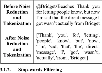
[image:5.612.314.521.378.526.2]Table 2 shows a sample of the dataset before and after performing the noise reduction and tokenization.
Table 1: Sample Results of Noise Reduction and Tokenization
Before Noise Reduction
and Tokenization
@BridgetsBeaches Thank you for letting people know, but now I’m sad that the direct message I got wasn’t actually from Bridget
After Noise Reduction
and Tokenization
['Thank', 'you', 'for', 'letting', 'people', 'know', 'but', 'now', 'I’m', 'sad', 'that', 'the', 'direct', 'message', 'I', 'got', 'wasn’t', 'actually', 'from', 'Bridget']
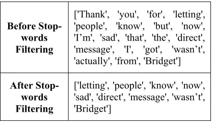
3.1.2. Stop-words Filtering
Stop-words filtering is a technique used in NLP to remove commonly occurring words in a language with little or no impact on the value of the target. Example of stop-words are demonstratives, prepositions or pronouns. To remove stop-words, we need a dictionary that contain all possible stop-words. Table 3 shows a sample of stop-words in the dictionary.
Table 2: Sample of Stop-words
Group Name Example
Demonstratives This – Those - These
Pronouns I - You - My
3502 To remove stop-words, we used the following algorithm:
Algorithm 5: Remove Stop-words
stop_word_filtering(word) 1 f Read Dictionary
2 stopword_list read f & splitlines() 3 for sw in stopword_list
4 if sw = word
5 return True
[image:6.612.313.524.87.213.2]6 return False
Table 4 shows a sample of the dataset before and after performing the stop-words filtering.
Table 3: Sample Result of Stop-Words Filtering
Before Stop-words Filtering
['Thank', 'you', 'for', 'letting', 'people', 'know', 'but', 'now', 'I’m', 'sad', 'that', 'the', 'direct', 'message', 'I', 'got', 'wasn’t', 'actually', 'from', 'Bridget']
After Stop-words Filtering
['letting', 'people', 'know', 'now', 'sad', 'direct', 'message', 'wasn’t', 'Bridget']
3.1.3. Stemming
Stemming is a technique used in NLP in order to remove morphological affixes or prefixes and retrieve the root of words. There are many stemmers for English such as Snowball, Porter and LancasterStemmer. The proposed solution used the Porter stemming since it’s simple and generates the root using suffix stripping. We used the following algorithm to apply the Porter Stemmer:
Algorithm 6: Stemming
stemming(word)
1 ps PorterStemmer() 2 word stem(word)
3 return word
[image:6.612.94.294.141.237.2]Table 5 shows a sample of the dataset after performing the Porter Stemmer.
Table 4: Sample Result of Porter Stemmer
Before Stemming
['letting', 'people', 'know', 'now', 'sad', 'direct', 'message', 'wasn’t', 'Bridget']
After
Stemming ['let', 'peopl', 'know', 'sad', 'direct', 'messag', 'wasn’t', 'bridget']
3.1.4. N-gram
N-gram model is a sequence of n-words. N represents the length of words per phase, it can be bi-gram, tri-gram or big-gram (i.e. n = 2, n = 3 or n > 3). N-gram usually used in SA to generate the words that have meaning together and will differ if we take them as a single word. Using n-gram will help in training the model and in the classification step.
3.2. Classification
The proposed solution uses two ML methods which are: Supervised Learning and CE. For the Supervised Learning, we used Multinomial NB and SVM classifiers. This section presents an overview of these classifiers.
3.2.1. Multinomial Naïve Bayes
We used a Multinomial NB classifier which is an effective classifier for text classification. The classifier used as following:
1. Split the data into training and testing (70% training and 30% testing).
2. Create the count vectorizer with the class CountVectorizer.
3. Create the TFIDF transformer with the class TfidfTransformer.
4. Create the Multinomial NB classifier with the class MultinomialNB.
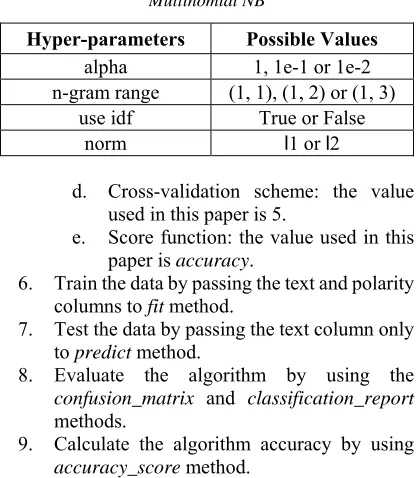
5. Use GridSearchCV to find the best parameters for the classifier by passing the following:
a. Estimator: in this paper the estimator consists of count vectorizer, TFIDF transformer and Multinomial NB classifier objects combined into one estimator using the class Pipeline. b. Hyper-parameters: alpha, n-gram
range, use idf and norm. Table 6 shows the possible values for each parameter.
[image:6.612.90.300.307.434.2]3503
Table 5: Possible Values for Each Hyper-parameter - Multinomial NB
Hyper-parameters Possible Values
alpha 1, 1e-1 or 1e-2
n-gram range (1, 1), (1, 2) or (1, 3)
use idf True or False
norm l1 or l2
d. Cross-validation scheme: the value used in this paper is 5.
e. Score function: the value used in this paper is accuracy.
6. Train the data by passing the text and polarity columns to fit method.
7. Test the data by passing the text column only to predict method.
8. Evaluate the algorithm by using the confusion_matrix and classification_report methods.
9. Calculate the algorithm accuracy by using accuracy_score method.
3.2.2. Support Vector Machine
SVM is one of the most common used classifiers for text classification. The classifier is used as following:
1. Split the data into training and testing (70% training and 30% testing).
2. Use GridSearchCV to find the best parameters for the classifier by passing the following:
a. Estimator: which is the classifier. Here we used SVC class.
b. Hyper-parameters: C, kernel, gamma and decision function shape. Table 7 shows the possible values for each parameter.
Table 6: Possible Values for Each Hyper-parameter - SVM
Hyper-parameters Possible values
C 0.25, 0.5, 0.75 or 1 kernel linear or rbf (Radial Basis Function)
gamma 1, 2, 3 or auto
decision function shape
ovo (one vs. one) or ovr (one vs. rest) c. Cross-validation scheme: the value
used in our study is 5.
d. Score function: the value used in this paper is accuracy.
3. Train the data by passing the text and polarity columns to fit method.
4. Test the data by passing the text column only to predict method.
5. Evaluate the algorithm by using the confusion_matrix and classification_report methods.
6. Calculate the algorithm accuracy by using accuracy_score method.
3.2.3. Classifier Ensemble
The chosen ensemble technique in this paper is boosting using AdaBoost classifier. AdaBoost algorithm starts by fitting the classifier on the initial dataset and gives all instances the same weight value. After that, it starts fitting additional versions of the base classifier on the same dataset, but each next version focuses on handling the misclassified instances more by assigning them a higher weight. We used the CE as following:
1. Split the data into training and testing (70% training and 30% testing).
2. Create the count vectorizer with the class CountVectorizer.
3. Create the TFIDF transformer with the class TfidfTransformer.
4. Create the Ada Boost classifier with the class AdaBoostClassifier.
5. Use GridSearchCV to find the best parameters for the classifier by passing the following:
a. Estimator: in this paper the estimator consists of count vectorizer, TFIDF transformer and Ada boost classifier objects combined into one estimator using the class Pipeline.
b. Hyper-parameters: base estimator, algorithm, number of estimators, n-gram range, use idf and norm. Table 8 shows the possible values for each parameter.
Table 7: Possible Values for Each Hyper-parameter - CE
Hyper-parameters Possible Values
base estimator MultinomialNB(1e-1) or MultinomialNB(1), MultinomialNB(1e-2) algorithm SAMME.R or SAMME number of
estimators Odd numbers from 1 to 50 n-gram range (1, 1), (1, 2) or (1, 3)
use idf True or False
3504 c. Cross-validation scheme: the value
specified for this study is 5.
d. Score function: the value specified for this paper is accuracy.
6. Train the data by passing the text and polarity columns to fit method.
7. Test the data by passing the text column only to predict method.
8. Evaluate the algorithm by using the
confusion_matrix and
classification_report methods.
9. Calculate the algorithm accuracy by using accuracy_score method.
4. EMPIRICAL STUDIES
This section describes the dataset by listing its features. Then, it presents the results for each classifier after applying the steps mentioned in the section Three.
4.1. Description of dataset
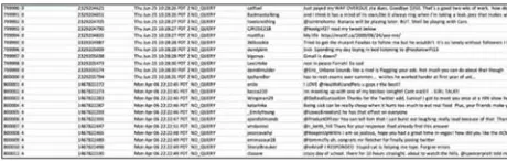
The dataset used in our study was collected and classified by Go et al. (24) It has six features as listed below:
1. The polarity of the tweet (0 for negative and 4 for positive).
2. The tweet ID.
3. Date (indicates the post date).
4. The query. If there is no query, then this value is NO_QUERY.
5. The username.
6. The content of the tweet.
[image:8.612.76.306.534.607.2]They used the Twitter Search API to collect their dataset using some keywords. Figure 1 shows a sample from the training dataset.
Figure 1: Sample from the Training Dataset
4.2. Experimental Setup
For investigating the performance of the proposed techniques confusion matrix, Precision, Recall, F1 Score and support is used. Finally, the classifiers are compared with the optimal preprocessing was compared in terms of sensitivity, specificity, Precision and Time Complexity Also, it
uses different preprocessing techniques for each classifier as specified in Table 9, Table 12 and Table 15. In each table, the first column is the run ID. The second column indicates whether stop-words filtering is applied (1) or not (0) in each run. The third column indicates whether stemming is applied (1) or not (0), and the fourth column indicates the used n-gram type. This section presents the experiment results for Multinomial NB, SVM and CE.
4.2.1. Multinomial Naïve Bayes
3505
Table 9: Multinomial NB Experiment Results
Classifier ID
Stop-words Filteri
ng
Stemmi ng
N-gram
Precisi on
Multinom
ial NB#1 1 1 Unigram 68.45 %
Multinom
ial NB#2 0 1
Unigra m, bigram
and trigram
78.01 %
Multinom
ial NB#3 0 0
Unigra m and bigram
78.14 %
Figure 2 illustrates the trial results of SA with the highest precision which is Multinomial NB#3.
Figure 2: SA Results of Multinomial NB#3
Table 10 shows the confusion matrix of Multinomial NB#3.
Table 10: Confusion Matrix of Multinomial NB#3
Predicted Class
Actual Class
- Class = 4 Class = 0 Class = 4 2084 933 Class = 0 583 2400
Table 11 shows the best hyper-parameters set for the Multinomial NB#3.
Table 11: Best Values for Each Hyper-parameter - Multinomial NB#3
Hyper-parameters Best Values
alpha 0.1
n-gram range (1, 2)
use idf False
norm l1
4.2.2. Support Vector Machine
Table 12 shows several trials using SVM classifier.
Table 12: SVM Experiment Results
Classifi er ID
Stop-words Filteri
ng
Stemmi ng
N-gra
m
Precisi on
SVM#1 1 1 0 60.17 %
SVM#2 0 1 0 55.65 %
SVM#3 0 0 0 54.26 %
Figure 3 illustrates the trial results of SA with the highest precision which is SVM#1.
Figure 3: SA Results of SVM#1
Table 13 shows the confusion matrix of SVM#1.
Table 13: Confusion Matrix of SVM#1
Predicted Class
Actual Class
- Class = 4 Class = 0 Class = 4 1509 1481 Class = 0 999 2011
Table 14 shows the best hyper-parameters set for the SVM#1.
Table 14: Best Values for Each Hyper-parameter – SVM#1
Hyper-parameters Best Values
C 0.75
kernel rbf
gamma 1
decision function
shape ovo
4.2.3. Classifier Ensemble
3506
Table 15: CE Experiment Results
Class ifier ID
Stop-word s Filte ring
Stem ming
N-gram
Preci sion
Time Compl exity
CE#1 1 1 Unigram 75.53 % 15069.7 sec
CE#2 0 1 Unigram 75.53 % 14666.4 sec
[image:10.612.90.298.94.234.2]CE#3 0 0 Unigram 75.53 % 14737.8 sec
[image:10.612.313.526.101.241.2]Figure 4 illustrates the trial results of SA with the best time complexity which is CE#2.
Figure 4: SA Results of CE#2
[image:10.612.91.298.285.358.2]Table 15 shows the confusion matrix of CE#2.
Table 15: Confusion Matrix of CE#2
Predicted Class
Actual Class
- Class = 4 Class = 0
Class = 4 2293 724
Class = 0 743 2240
[image:10.612.88.301.418.485.2]Table 16 shows the best hyper-parameters set for the CE#2.
Table 16: Best Values for Each Hyper-parameter – CE#2
Hyper-parameters Best Values
n-gram range (1, 1)
use idf True
norm l2
base estimator MultinomialNB(1e-2)
algorithm SAMME.R
number of estimators 45
Table 17 shows the assessment of best trial for each classifier.
Table 17: Comparison of the MNB, SVM and CE models
Classifi
er ID Sensitivity Specificity Precision
Time Compl exity Multino
mial NB#3
69.08
% 80.46 % 78.14 % 447.2 sec
SVM#1 50.47 % 66.81 % 60.17 % 8466.1 sec
CE#2 76 % 75.09 % 75.53 % 14666.4 sec
Starting with Multinomial NB#3, it gave us the highest precision value without stop-word filtering and stemming techniques with the use of unigram and bigram. In case of SVM#1, it gave us a high value of precision when we applied both stop-word filtering and stemming. The last classifier which is CE#2, it results with the same performance, but different time complexity and criteria was based on the best time complexity trial. To conclude the discussion, Multinomial NB#3 gave us the highest precision value among other classifiers. By comparing with time complexity, Multinomial NB#3 has the minimum time complexity with value 447.2 sec, unlike CE#2 that has the highest value among other classifiers.
5. CONCLUSION
[image:10.612.90.299.560.668.2]3507 classifier perform different with different preprocessing techniques like NMB achieves the highest precision without stemming and stop word removal wile SVM accuracy is increased after applying both the preprocessing modules i.e. stemming and stop word removal. The selection of the preprocessing module is also dependent on the classifiers specifically in the sentiment analysis as the tweets are highly unstructured.
REFERENCES
[1]
https://www.statista.com/statistics/617136 /digital.
[2] Joshi N, Itkat S. A Survey on Feature Level Sentiment Analysis. Int J Comput Sci Inf Technol. 2014;5(4):5422–5.
[3] Ismail HM, Belkhouche B, Zaki N. Semantic Twitter sentiment analysis based on a fuzzy thesaurus. Soft Comput [Internet]. 2018;22(18):6011–24.
Available from:
https://doi.org/10.1007/s00500-017-2994-8
[4] A. V, Sonawane SS. Sentiment Analysis of Twitter Data: A Survey of Techniques. Int J Comput Appl. 2016;139(11):5–15. [5] Khan FH, Bashir S, Qamar U. TOM:
Twitter opinion mining framework using hybrid classification scheme. Decis Support Syst [Internet]. 2014;57(1):245–
57. Available from:
http://dx.doi.org/10.1016/j.dss.2013.09.00 4
[6] Rehioui H, Idrissi A. New Clustering Algorithms for Twitter Sentiment Analysis. IEEE Syst J. 2019;PP:1–8.
[7] Ashna MP, Sunny AK. Lexicon based sentiment analysis system for malayalam language. Proc Int Conf Comput Methodol Commun ICCMC 2017. 2018;2018-Janua(Iccmc):777–83.
[8] Giachanou A, Crestani F. Like it or not: A survey of Twitter sentiment analysis methods. ACM Comput Surv. 2016;49(2). [9] Rojas-Barahona LM. Deep learning for
sentiment analysis. Lang Linguist Compass. 2016;10(12):701–19.
[10] Lima ACES, De Castro LN, Corchado JM. A polarity analysis framework for Twitter messages. Appl Math Comput [Internet]. 2015;270:756–67. Available from: http://dx.doi.org/10.1016/j.amc.2015.08.0 59
[11] Zhang Y, Song D, Zhang P, Li X, Wang P. A quantum-inspired sentiment representation model for twitter sentiment analysis. Appl Intell. 2019;49(8):3093– 108.
[12] Zamani NAM, Abidin SZZ, Omar N, Abiden MZZ. Sentiment analysis: Determining people’s emotions in facebook. Proc 13th Int Conf Appl Comput Appl Comput Sci. 2014;111–6.
[13] Uryupina O, Plank B, Severyn A, Rotondi A, Moschitti A. SenTube: A corpus for sentiment analysis on YouTube social media. Ninth Int Conf Lang Resour Eval. 2014;2:4244–9.
[14] Uryupina O, Plank B, Severyn A, Rotondi A, Moschitti A. SenTube: A corpus for sentiment analysis on YouTube social media. Proc 9th Int Conf Lang Resour Eval Lr 2014. 2014;2:4244–9.
[15] Gautam G, Yadav D. Sentiment analysis of twitter data using machine learning approaches and semantic analysis. 2014 7th Int Conf Contemp Comput IC3 2014. 2014;(October 2015):437–42.
[16] Wan Y, Gao Q. An Ensemble Sentiment Classification System of Twitter Data for Airline Services Analysis. Proc - 15th IEEE Int Conf Data Min Work ICDMW 2015. 2016;1318–25.
[17] Hu M, Liu B. Mining and summarizing customer reviews. Proc 2004 ACM SIGKDD Int Conf Knowl Discov data Min - KDD ’04. 2004;168.
[18] Alsaeedi A. EFTSA: Evaluation Framework for Twitter Sentiment Analysis. J Softw. 2019;14(1):24–35.
[19] Jo K, Eds LW, Goebel R. Computing. 2014.
[20] Haddi E, Liu X, Shi Y. The role of text pre-processing in sentiment analysis. Procedia Comput Sci [Internet]. 2013;17:26–32.
Available from:
http://dx.doi.org/10.1016/j.procs.2013.05. 005
[21] Rasool A, Tao R, Marjan K, Naveed T. Twitter Sentiment Analysis: A Case Study for Apparel Brands. J Phys Conf Ser. 2019;1176(2).
3508 [23] Symeonidis S, Effrosynidis D, Arampatzis
A. A comparative evaluation of pre-processing techniques and their interactions for twitter sentiment analysis. Expert Syst Appl [Internet]. 2018;110:298–310. Available from: https://doi.org/10.1016/j.eswa.2018.06.02 2