Some comments on goodness-of-fit tests for the parametric form of the copula based on L^2-distances

(1)

SFB

823 Some comments on

Some comments on

goodness

goodness----of

of

of----fit tests for the

of

fit tests for the

parametric form of the copula

based on

_L

2

2 ----distances

distances

D

is

c

u

s

io

n

P

a

p

e

r

Axel Bücher, Holger Dette,

(2)

(3)

Some comments on goodness-of-fit tests for the parametric

form of the copula based on

L

2 -distances

Axel B¨ucher

Ruhr-Universit¨at Bochum

Fakult¨at f¨ur Mathematik

44780 Bochum, Germany

e-mail: [email protected]

Holger Dette

Ruhr-Universit¨at Bochum

Fakult¨at f¨ur Mathematik

44780 Bochum, Germany

email: [email protected]

6 July 2009

Abstract

In a recent paper Fermanian (2005) studied a goodness-of-fit test for the parametric form of a copula, which is based on an L2_{-distance between a parametric and nonparametric}

estimate of the copula density. In the present paper we investigate the asymptotic properties of the proposed test statistic under fixed alternatives. We also study the impact of different estimates for the parameters of the finite dimensional family of copulas specified by the null hypothesis and illustrate the performance of a parametric bootstrap procedure for the approximation of the critical values.

Keywords and Phrases: goodness-of-fit tests, Copula, L2_{-distance, parametric bootstrap}

AMS Subject Classification: 62G; 62P

1 Introduction

Nowadays copulas are widely used by practitioners to analyze dependence structures in various applications including finance, actuarial science and hydrology [see e.g. Frees and Valdez (1998), Embrechts, McNeil and Straumann (2002), McNeil, Frey and Embrechts (2005) and Genest and Favre (2007)]. The copula of a multivariate distribution describes its dependence structure as a complement to the behaviour of its margins, and as a consequence the estimation of the distribution can be splitted into the estimation of the marginals and the copula. Several parametric families of copulas

C ={Cθ |θ ∈Θ}

(4)

(here Θ⊂Rq _{denotes an arbitrary subset) have been proposed in the literature in order to reflect}

various aspects of dependency [see e.g. the monographs of Joe (1997) or Nelsen (2006)]. Because misspecification of the copula function can have a serious impact on the statistical analysis, several authors have pointed out the importance of goodness-of-fit tests for the hypothesis of a parametric family (1.1) [see e.g. Malevergne and Sornette (2003), Cui and Sun (2004), Fermanian (2005), Scaillet (2007), Dobric and Schmid (2007), Genest and R´emillard (2008) among many others]. In a recent paper Fermanian (2005) proposed a test for the hypothesis

H0 :C∈ C , H1 : C /∈ C

(1.2)

where C denotes the copula of a d-dimensional distribution and C the parametric class defined by (1.1). The test is based on an L2_{-distance between a nonparametric and parametric estimate of}

the copula density, and Fermanian (2005) proved asymptotic normality of the corresponding test statistic under the null hypothesis H0 and specific assumptions on the estimates of the parameters

of the copula density.

The present paper has several purposes. First we provide a more sophisticated analysis of the test proposed by Fermanian (2005) and study the asymptotic properties of the test statistic under fixed alternatives. It is shown that in this case an appropriately standardized version of the test statistic is also asymptotically normal distributed. Moreover, in contrast to the null hypothesis, it turns out that under the alternative the form of the parametric estimate has a substantial impact on the asymptotic distribution of the test statistic. In particular, we investigate two estimation methods for the parameter of the copula density, namely the common maximum likelihood and minimumL2_{-distance estimation technique. For these estimates we prove asymptotic normality of}

the standardized test statistic under the null hypothesis and fixed alternatives with different rates of convergence in both cases. These results can be used for the construction of confidence regions for a measure of deviation, say M2_{, between the parametric family of copulas and the ”true”}

copula or for testing precise hypotheses of the form H0 : M2 ≤∆ vs. H1 : M2 >∆, where ∆≥ 0

is a preassigned measure of accuracy [see Berger and Delampady (1987)]. These hypotheses are motivated by the observation that in practice a copula will never be exactly of a given parametric form (which would correspond to the case ∆ = 0), but in the best case approximately given by a parametric form (which would correspond to a small value of ∆).

Secondly it has been pointed out by several authors that under the null hypothesis the normal approximation of test statistics based on L2_{-distances is not very accurate [see e.g. H¨ardle and}

Mammen (1993) or Fan and Linton (2003)]. Therefore we propose a parametric bootstrap pro-cedure for the approximation of the critical values and investigate its performance by means of a simulation study. In particular, it is demonstrated that the bootstrap test based on theL2_-distance

yields a reliable approximation of the nominal level and has similar power properties as several goodness-of-fit tests, which were investigated in a recent paper by Genest, R´emillard and Beaudoin (2008).

The remaining part of the paper is organized as follows. In Section 2 we introduce the necessary notation and define the test statistic. The asymptotic properties of the maximum likelihood and the minimum L2_{-distance in the parametric family of copulas are investigated in Section 3 under}

(5)

a correct and incorrect specification of the parametric family of copulas. In Section 4 we prove asymptotic normality of the test statistic under the null hypothesis and fixed alternatives with different rates of convergence in both cases. Section 5 is devoted to a small simulation study in order to investigate the finite sample properties of a parametric bootstrap procedure based on the

L2_{-distance. Finally, some more technical results are presented in the Appendix.}

2 Testing for the form of the copula with the

L

2

-distance

Throughout this paper let X1, . . . , Xn denote independent identically distributed d-dimensional

random variables with joint continuous distribution functionH and copulaC, which has a density

τ0 supported in the cube [0,1]d. We denote byXi = (Xi,1, . . . , Xi,d)T the components of the vector

Xi(i= 1, . . . , n) and by Fj the marginal distribution of the jth component (j = 1, . . . , d), which

yields by Sklar’s theorem [see e.g. Nelsen (2006)]

H(x1, . . . , xd) =C(F1(x1), . . . , Fd(xd)) a.e.. (2.1) We define by Fn,r(x) = 1 n n X j=1 1{Xj,r ≤x} (2.2)

the empirical distribution function of the r-th marginal distribution Fr (r= 1, . . . , d) and

Yi := (F1(Xi,1), . . . , Fd(Xi,d))T

(2.3)

Yn,i := (Fn,1(Xi,1), . . . , Fn,d(Xi,d))T,

(2.4)

(note that the distribution function of the random variable Yi is given by the copula C). We

assume for the parametric class of copulas defined by (1.1) that the parameter space Θ is compact with non empty interior and thatCθ has a density supported in [0,1]d, sayτ(·, θ), which is two and

three times continuously differentiable with respect to the first and second argument, respectively. In the following discussion ˆθ denotes an (under the null hypothesis consistent) estimate of the parameter θ, which will be specified in the following section, and we denote by ˆτ(·) = τ(·,θˆ) the corresponding parametric estimate of the copula density. Moreover, the nonparametric kernel estimate of the copula density is defined by

τn(u) := 1 nhd n X i=1 K µ u−Yn,i h ¶ (2.5)

[see e.g. Charpentier, Fermanian and Scaillet (2007)] and ω : [0,1]d _−→ _IR+

0 denotes a two

times continuously differentiable weight function with compact support contained in the cube [ε1,1−ε1]d ⊂ [0,1]d, where ε1 > 0. We further assume that τ(·,·) is uniformly continuous on

(6)

[ε0,1−ε0]d×Θ for some ε0 ∈(0, ε1). For testing the parametric hypothesis (1.2) Fermanian (2005)

proposed the test statistic

Jn=Jn(bθ) :=

Z

(τn−Kh∗τb)2(u)ω(u)du.

(2.6)

where ∗ denotes convolution and Kh(x) = K(x/h)/h. Here K denotes the kernel of the density

estimate (2.5), and the convolution operator is applied to the parametric estimate of the copula density in order to reduce the bias [see e.g. Bickel and Rosenblatt (1973) or H¨ardle and Mammen (1993)]. Because the asymptotic properties of the test statistic, especially under a fixed alternative, depend sensitively on the specific choice of the parametric estimate, we study in the following section two estimation methods for the parameter θ of the family of copula densities.

3 Estimation of the parameter of the copula density

Throughout this paper let τ0 denote the “true” density of the copula C and consider the Kulback

Leibler distance DKL(τ0, τ(·, θ)) = Z log(τ0(u))τ0(u)du− Z log(τ(u, θ))τ0(u)du, (3.1)

We define L(θ) =R logτ(u, θ)τ0(u)du and

θ∗

M L = argmax θ∈Θ

L(θ)

(3.2)

as the parameter corresponding to the best approximation of the copula density τ0 by the

para-metric class {τ(·, θ) | θ ∈ Θ} with respect to the Kulback Leibler distance and assume that θ∗

M L

is attained at an unique interior point of Θ. The maximum likelihood estimate of the parameter

θ is defined as b θM L := argmax θ∈Θ Ln(θ). (3.3) whereLn(θ) := 1_n P_n

i=1logτ(Yn,i, θ) denotes the likelihood function [see Genest, Ghoudi and Rivest

(1995)]. We assume that ˆθM L is also attained at an interior point of the parameter space Θ and

that the parametric class of copula densities satisfies the following assumptions of regularity: (a) E£k∂θlogτ(Yi, θM L∗ )k+ ° °_∂2 yθlogτ(Yi, θ∗M L) ° °₊°°_∂3 yyθlogτ(Yi, θM L∗ ) ° °¤_<_∞

(b) There exist constants α, β >0, such that for any point Y∗

ni with kYni∗ −Yik ≤ kYni−Yik ° °_∂3 yyθlog(Yni∗, θ∗M L) ° °_≤_α°°_∂3 yyθlogτ(Yi, θML∗ ) ° °₊_β°°_∂3 yyθlogτ(Yni, θM L∗ ) ° °

(c) For all u∈(0,1)d _{we have with the notation} _r₍_t_{) :=} _t₍₁₋_t₎

° °_∂3 yyθlogτ(u, θ∗M L) ° °_≤_{const r}₍_u₁₎a1_{. . . r}₍_u d)ad,

(7)

(d) For all u∈(0,1)d ° °_∂2 θθlogτ(u, θ∗M L) ° °_≤_{const r}₍_u₁₎b1_{. . . r}₍_u d)bd, where bk = ζ_q−_k1 and _q1₁ +· · ·+_q1_d = 1, ζ >0.

(e) For all u∈(0,1)d _{we have in a neighbourhood}_V₍_θ∗

M L) of the point θM L∗ sup θ∈V(θ∗ M L) ° °_∂3 θθθlogτ(u, θ) ° °_≤_{const r}₍_u₁₎c1_{. . . r}₍_u d)cd, where ck = η_p−01 k and 1 p0 1 +· · ·+ 1 p0 d = 1, η >0.

Fermanian (2005) states that these assumptions are satisfied for most of the commonly used copula families [see also Hu (1998), who proved some of these assumptions for Clayton-, Frank- and Gauß-copulas]. Our first result establishes a stochastic expansion for the maximum likelihood estimate, from which asymptotic normality can be derived.

Theorem 3.1. If the assumptions stated in Section 2 and 3 are satisfied and the maximum

likelihood estimate θˆM L is consistent, i.e. θˆM L −→P θ∗M L, then

√ n(θbM L−θM L∗ ) = 1 √ n n X i=1 D(Yi) +oP(1) −→ ND (0,Σ), (3.4) where D(Yi) = A−1(∂θlogτ(Yi, θ∗M L) +h(Yi)), h(Yi) = Z ∂2

yθlogτ(u, θM L∗ )(1(Yi ≤u)−u)τ0(u)du,

A = −E£∂_θ2logτ(Yi, θM L∗ )

¤

,

Σ = Var(D(Yi)).

Proof. The proof follows by similar arguments as presented in part D of the paper by Fermanian (2005). Because this author only considers the null hypothesis and some of the arguments in this reference seem to be incorrect (see our Remark 3.2), we present here the main steps. Because ˆθML

is an interior point of the parameter space, we obtain by means of Taylor expansions 0 = ∂θLn(θbM L) = S0 +S1+S2 (3.5) +∂2 θθLn(θM L∗ ) (θbM L−θM L∗ ) + 1 2(bθM L−θ ∗ M L)T∂θθθ3 Ln(˜θ) (bθM L−θ∗M L),

where the terms S0, S1, S2 are defined by

S0 = 1 n n X i=1 ∂θ logτ(Yi, θ∗M L), (3.6) S1 = 1 n n X i=1 ∂2

yθ logτ(Yi, θM L∗ )(Yn,i−Yi),

(3.7) S2 = 1 2n n X i=1

(Yn,i−Yi)T ∂yyθ3 logτ(Yn,i∗ , θM L∗ ) (Yn,i−Yi),

(8)

and ˜θ and Y∗ ni satisfy kθ˜−θ∗M Lk ≤ kθˆM L −θˆ∗M Lk and ° °_Y∗ n,i−Yi ° ° _{≤ k}_Y_n,i₋_Y_i_k ₍_i _{= 1}_{, . . . , n}_),

respectively. Note thatE[S0] = 0 and thereforeS0 is a sum of centered, independent and identically

distributed random variables. Using a Hoeffding approximation it follows for the second term

S1 = 1 n n X i=1 h(Yi) +oP µ 1 √ n ¶ , (3.9)

where the random variableh(Yi) is defined in Theorem 3.1. Finally, we have (using the assumptions

(a) - (c)) that S2 =OP(log_n2n) =oP(√1_n). Combining these estimates we obtain

∂θLn(θ∗M L) =S0+S1+S2 = 1 n n X i=1 A·D(Yi) +oP µ 1 √ n ¶ , (3.10)

where we have again used the notation of Theorem 3.1. Note that it follows from Proposition A.1 in Genest, Ghoudi and Rivest (1995) that ∂2

θθLn(θ∗M L) P

→ −A, which implies (observing that

∂3

θθθLn(˜θ) is bounded in probability, because of assumption (e) and ˜θ→P θ∗M L)

−∂θLn(θ∗M L) = (−A+oP(1)) (bθML−θ∗M L)

(3.11)

The assertion of the Theorem now follows from (3.5) and (3.10) by a standard argument. 2

Remark 3.2.

(a) Note that Theorem 3.1 requires the consistency of the maximum likelihood estimate ˆθM L →P

θ∗

M L, where θ∗M L is the best approximation of the “true” copula density τ0 by the parametric

class {τ(·, θ)|θ ∈Θ} with respect to the Kulback Leibler distance. If the parametric model has been correctly specified, this was proved in Theorem 4.2.1 of Hu (1998) and similar arguments could be used to establish consistency of ˆθML if the model has been misspecified.

(b) It should be pointed out here that Fermanian (2005) considered estimates of the parameter

θ satisfying ˆ θ−θ0 = 1 nA −1₍_θ 0) n X i=1 B(θ0, Yi) +op(n−1/2(logn)−1/2)

whereθ0 is the “true” parameter of the copula (this means that the model has been correctly

specified). However, we were not able to find estimates in the literature satisfying this assumption (in particular the proof presented in Appendix D of Fermanian (2005) seems to be not correct).

In the remaining part of this section we derive a similar expansion for an estimate minimizing an

L2_{-distance between the “true” copula density and the parametric class of densities specified by}

the null hypothesis. To be precise we define

θ∗ L2 := argmin θ∈Θ Z _¡ τ(u, θ)−τ0(u) ¢₂ ω(u)du (3.12)

(9)

as the parameter corresponding to the bestL2_{-approximation of}_τ

0by the parametric class{τ(·, θ)|θ ∈

Θ}and we assume that it is attained at an unique interior point of the parameter space Θ. If the model is correctly specified andθ0 the true parameter corresponding to the densityτ0(·) =τ(·, θ0),

then θ∗

L2 =θ0. The empirical analogue of (3.12) is given by

b θL2 = argmin θ∈Θ Z _¡ τ(u, θ)−τn(u) ¢₂ ω(u)du , (3.13)

where τn denotes the kernel estimate of the copula defined by (2.5). The following result provides

a stochastic expansion for the difference ˆθL2 −θ∗_L2.

Theorem 3.3. If the L2_{-estimate is consistent, i.e.} _θˆ

L2 −→P θ∗

L2, and the conditions h −→ 0,

nhd_{−→ ∞}_, log2₂n nh4+d 2 −→ 0 (3.14) log(h−d₎ nhd → 0 (3.15) log(h−d₎ log₂n → ∞ (3.16) n1−α_hd _{−→ ∞} (3.17)

are satisfied for some α∈(0,3

4), then it follows that

b θL2 −θ_L∗2 +B = 1 n n X i=1 Dn(Yi) + oP( 1 √ n), (3.18)

where the bias is given by

B := Z (Kh∗τ0(u)−τ0(u))C−1∂θτ(u, θ∗L2)ω(u)du=O(h2). (3.19) and δ(u) := τ(u, θ∗ L2)−τ₀(u) (3.20) C = Z {∂θτ(u, θL∗2)∂_θTτ(u, θ_L∗2) +δ(u)∂_θθ2 τ(u, θ∗_L2)}ω(u)du. (3.21) Dn(Yi) := C−1 ·Z (Kh(u−Yi)−E[Kh(u−Yi)])∂θτ(u, θ∗L2)ω(u)du+r_n(Y_i) ¸ (3.22) rn(Yi) := E[hn(Yk, Yi)|Yi] (3.23) hn(Yk, Yi) := −1 h Z (dK)_h(u−Yk)(1(Yi ≤Yk)−Yk)∂θτ(u, θ∗L2)ω(u)du. (3.24) In particular, we have 1 √ n n X i=1 Dn(Yi)−→ ND q(0,Σ), (3.25)

(10)

where the asymptotic variance is given by Σ = C−1_E · ∂θτ(Yi, θL∗2)∂_θTτ(Y_i, θ∗_L2)ω2(Y_i) (3.26) −E[∂θτ(Yi, θ∗L2)ω(Y_i)] E £ ∂T θ τ(Yi, θL∗2)ω(Y_i) ¤ −2 d X r=1 Z ∂θτ(Yi, θ∗L2)ω(Y_i) (τ₀∂_θTτ(·, θ∗_L2)ω)(v₁, . . . , Y_ir. . . , v_d)dv₋_r + d X r,s=1 Z (τ0∂θ(·, θL∗2)ω)(u₁, . . . , Y_ir, . . . , u_d)(τ₀∂_θT(·, θ∗_L2)ω) (v1, . . . , Yis, . . . , vd)du−rdv−s ¸ C−1

and the symbol du₋_r means integration with respect to the (d −1)-dimensional variable u₋_r =

(u1, . . . , ur−1, ur+1, . . . , ud).

Proof. With the notation

Qn(θ) = − Z _¡ τ(u, θ)−τn(u) ¢₂ ω(u)du, Q(θ) = − Z _¡ τ(u, θ)−τ0(u) ¢₂ ω(u)du, ψn(θ) = ∂θQn(θ) ψ(θ) = ∂θQ(θ)

we obtain for same ˜θ with kθ˜−θ∗

L2k ≤ kθˆL2 −θ_L∗k the expansion 0 = ∂θQn(θbL2) =∂_θQ_n(θ∗_L2) +∂2 θQn(θ∗L2) (θb_L2 −θ_L∗2) + 1 2(θbL2 −θ ∗ L2)T∂_θ3Q_n(˜θ) (θb_L2 −θ_L∗2). (3.27) Moreover, ∂θQn(θ∗L2) = 2 n n X i=1 Z _¡ Kh(u−Yn,i)−τ(u, θL∗2) ¢ ∂θτ(u, θ∗L2)ω(u)du (3.28) = 2 µ An1+An2+An3+An4 ¶ ,

(11)

where the random variables Anj (j = 1, . . . ,4) are defined by An1 = 1 n n X i=1 Z (Kh(u−Yi)−(Kh ∗τ0)(u))∂θτ(u, θL∗2)ω(u)du, An2 = 1 n n X i=1 Z βni(u)∂θτ(u, θL∗2)ω(u)du, An3 = 1 n n X i=1 Z γ∗ ni(u)∂θτ(u, θL∗2)ω(u)du, An4 = Z (Kh∗τ0(u)−τ(u, θ∗L2))∂_θτ(u, θ∗_L2)ω(u)du, and αi(u) := Kh(u−Yi), (3.29) βni(u) := −1 h (dK)h(u−Yi)(Yn,i−Yi), γ∗ ni(u) : = 1 2h2(d 2_K₎ h(u−Yn,i∗ )(Yn,i−Yi)(2).

Heredj_K _{denotes the}_j_{th derivative of the kernel}_K_{(note that}_K

h(u−Yni) =αi(u)+βni(u)+γni∗ (u)).

Observing the estimate kYn,i−Yik_∞ = OP

¡

(log2_nn)12

¢

it follows that An3 = Op(log2_nh2n) = op(√1_n).

For the term An2 we obtain by a straightforward but tedious calculation (see Appendix A)

An2 = 1 n n X i=1 rn(Yi) +op( 1 √ n), (3.30)

where we used the notation in (3.23). Finally,An4 =O(h2) by a standard calculation, which yields

∂θQn(θL∗2)−2 Z (Kh∗τ0(u)−τ0(u))∂θτ(u, θ∗L2)ω(u)du= 2 n n X i=1 C Dn(Yi) + oP( 1 √ n), (3.31)

where the matrix C is defined in (3.21). Under the assumptions of Theorem 3.3 it can be shown that the kernel estimate of the copula density converges uniformly in probability to the “true” density τ0 on [ε,1−ε]d (for anyε >0), and it follows

∂2 θQn(θL∗2) = 2 Z µ_¡ τn(u)−τ(u, θ∗L2) ¢ ∂2 θθτ(u, θ∗L2)−∂_θτ(u, θ∗_L2)∂_θTτ(u, θ∗_L2) ¶ ω(u)du P −→ −2C. (3.32)

Observing (3.27) this gives

∂θQn(θL∗2) = 2 ¡ C+oP(1) ¢ (bθL2 −θ_L∗2). (3.33)

(12)

and the assertion (3.18) follows because the matrix C is positive definite (note that θ∗

L2 minimizes

the function Q(θ) andθ∗

L2 is an interior point of Θ).

Note that the dominating term of the right hand side of (3.18) is a sum of centered i.i.d. random variables and the asymptotic normality now follows from the central limit theorem for triangular arrays and the Cram´er-Wold device. For the calculation of the asymptotic covariance we note that

Σn =E £ Dn(Yi)Dn(Yi)T ¤ = C−1_E£_{C D} n(Yi)(C Dn(Yi))T ¤ C−1 (3.34) = C−1{E_D(1)+ 2E_D(2)+E_D(3)}C−1, where E_D(1) = E£ Z (Kh(u−Yi)−E Kh(u−Yi))∂θτ(u, θL∗2) (Kh(v−Yi)−E Kh(v−Yi))∂θT τ(v, θL∗2)ω(u)ω(v)du dv ¤ , 2E_D(2) = E£ Z (Kh(u−Yi)−E Kh(u−Yi))∂θτ(u, θL∗2)ω(u)du r_nT(Y_i) ¤ , E_D(3) = E£rn(Yi)rTn(Yi) ¤ .

The assertion of the theorem now follows by a straightforward but tedious evaluation of the ex-pressions E_D(j) (j = 1,2,3) observing that

rn(Yi) =− d X i=1 Z (τ0∇τ(·, θL∗2)ω)(u₁, . . . , u_r₋₁, Y_ir, u_r₊₁, . . . , u_d)du₋_r,+O(h) 2

Remark 3.4. If the condition

k∂θQ(θ)|θ=θ∗

L2 k<inf{k∂θQ(θ)k |θ∈Θ;kθ−θ

∗

L2k ≥ε}

is satisfied for all ε > 0, then it has been shown by B¨ucher (2008) (using Theorem 5.9 in van der Vaart (1998)) that under the bandwidth conditions stated in Theorem 3.3 the estimate ˆθL2 is

consistent, that is ˆθ_L2 −→P θ_L∗2.

4 Weak convergence of the statistic

J

_n

(ˆ

θ

)

In this section we study the asymptotic properties of the goodness-of-fit test for the parametric form of the copula which is based on the L2_-distance _J

n with the estimator ˆθML or ˆθL2. We begin

with a statement of the asymptotic properties of the statistic Jn(ˆθ) under the null hypothesis of a

correct specification of the copula family.

Theorem 4.1. If the assumptions stated in Section 2 and 3 are satisfied and

nhd→ ∞, log 2 2n nh4+d 2 →0

(13)

, then nhd2 µ Jn(ˆθM L)− 1 nhd Z K2₍_t₎_τ 0(u−ht)ω(u)dt du+ 1 nh Z τ2 0ω d X r=1 Z K2 r ¶ DH0 −→ N(0,2σ2₎_, (4.1)

where the asymptotic variance is given by

σ2 ₌ Z τ2 0ω(u)du Z µZ K(u)K(u+v)du ¶₂ dv. (4.2) If additionally nh4+d _→₀_, _nh6+d₂ _→₀_{, then} nhd2 µ Jn(ˆθL2)− 1 nhd2 Z K2(t)τ0(u−ht)ω(u)dt du+ 1 nh Z τ₀2ω d X r=1 Z K_r2 − Z _¡ ∂T θτ(u, θ0)B ¢₂ ω(u)du ¶ DH₀ −→ N(0,2σ2₎_,

where σ2 _{is given as above and}

B = Z (Kh∗τ0(u)−τ0(u))C−1∂θτ(u, θ0)ω(u)du=O(h2), (4.3) C = Z ∂θτ(u, θ0)∂θTτ(u, θ0)ω(u)du.

The proof of this result follows by similar arguments as given by Fermanian (2005), where some modifications are necessary, because the estimators ˆθM L and ˆθL2 do not satisfy the assumptions

(3.1) of this paper. The details are omitted for the sake of brevity.

We now concentrate on the corresponding results under fixed alternatives.

Theorem 4.2. If the assumptions of Theorem 4.1 are satisfied and the null hypothesis is not valid,

that is τ0(·)6=τ(·, θ) for all θ ∈Θ, then

√ n µ Jn(ˆθM L)−b1 ¶ DH₁ −→ N(0, σ2 H1).

where the bias is given by

b1 =

Z

(Kh∗(τ0−τ∗))2(u)ω(u)du.

The asymptotic variance is given by

σ2

(14)

where σ11 := Var((τ0−τ∗)ω(Yi)), σ12 := −E · (τ0−τ∗)(Yi)ω(Yi) d X r=1 Z (τ0−τ∗)τ0ω(u1, . . . , Yir, . . . , ud)du−r ¸ , σ13 := βM LT A−1E · (τ0−τ∗)ω(Yi) µ ∂θlogτ(Yi, θ∗M L) +∂2 yθlogτ(Yj, θ∗M L)(1(Yi ≤Yj)−Yj) ¶¸ , σ22 := E · _Xd r,s=1 Z (τ0−τ∗)τ0ω(u1, . . . , Yir, . . . , ud) (τ0−τ∗)τ0ω(v1, . . . , Yis, . . . , vd)du−rdv−s ¸ , σ23 := βM LT A−1E · X r=1d Z (τ0−τ∗)τ0ω(v1,· · · , Yir,· · · , vd)dv−r µ

∂θlogτ(Yi, θ∗M L) +∂yθ2 logτ(Yj, θM L∗ )(1(Yi ≤Yj)−Yj)

¶¸

,

σ33 := βM LT Var(D(Yi))βM L

and we have used the notation τ∗₍_u_{) =} _τ₍_{u, θ}∗

M L), βM L = Z (τ0−τ∗)ω(u)∂θτ(u, θM L∗ )du. Similarly, we have √ n µ Jn(ˆθL2)−b₁−2b₂ ¶ DH₁ −→ N(0, σ_H2₁), where b1 = Z (Kh∗(τ0−τ∗))2(u)ω(u)du, b2 = Z Kh(u−t)(τ0−τ∗)(t)Kh(u−s)∂Tθτ(s, θL∗2)B ω(u)du ds dt =O(h3), σ2 H1 = 4(σ11+σ22+ 2σ12),

(15)

with σ11 := Var((τ0−τ∗)ω(Yi)), σ12 := −E ·_Xd r=1 Z (τ0−τ∗)τ0ω(u1, . . . , Yir, . . . , ud)(τ0−τ∗)(Yi)ω(Yi)du−r ¸ , σ22 := E · _Xd r,s=1 Z (τ0−τ∗)τ0ω(u1, . . . , Yir, . . . , ud) (τ0−τ∗)τ0ω(v1, . . . , Yis, . . . , vd)du−rdv−s ¸ .

Remark 4.3. Note that the choice ω(·) = τ(·, θ∗

M L)−1 yields βM L = Z τ0(u) ∂θ τ(u, θM L∗ ) τ(u, θ∗ M L) du− Z ∂θ τ(u, θ∗M L)du = Z τ0(u)∂θlogτ(u, θ)|θ=θ∗ M L du

and the term βML in the first part of Theorem 4.2 vanishes. By a careful inspection of the proof

of Theorem 4.2 it can be shown that for the choice ω(·) =τ(·,θˆM L)−1 the asymptotic variance of

the statistic √n(Jn(ˆθM L)−b1) simplifies substantially and is given by

σ2

H1 = 4(σ11+ 2σ12+σ22).

Proof of Theorem 4.2. We restrict ourselves to a proof of the first part, the corresponding result for the estimator ˆθL2 is derived similarly [see B¨ucher (2008)]. We use the decomposition

(4.4) Jn(ˆθM L) = Wn1+Wn2+Wn3+Wn4+Wn5+Wn6,

where the quantities Wnj are given by

Wn1 = Z (τn−Kh∗τ0)2(u)ω(u)du, Wn2 = Z (Kh∗(τ0−τ∗))2(u)ω(u)du, Wn3 = Z (Kh∗(τ∗−bτ))2(u)ω(u)du, Wn4 = 2 Z (τn−Kh∗τ0)(u)(Kh∗(τ0−τ∗))(u)ω(u)du, Wn5 = 2 Z (τn−Kh∗τ0)(u)(Kh∗(τ∗−bτ))(u)ω(u)du, Wn6 = 2 Z (Kh∗(τ0−τ∗))(u)(Kh∗(τ∗−bτ))(u)ω(u)du,

(16)

τ∗₍_·_{) =}_τ₍_·_{, θ}∗

M L) denotes the best approximation of the “true” copula density τ0 by the parametric

family with respect to the Kulback Leibler distance and ˆτ(θ) = τ(·,θˆM L) its corresponding estimate.

From the proof of Theorem 4.1 [see Fermanian (2005)] we obtain

Wn1 =op(n−1/2), Wn3 =op(n−1/2),

and the assertion of the theorem follows, if the weak convergence

√

n (Wn4+Wn5+Wn6)−→ ND (0, σH21)

(4.5)

can be established. In order to prove this result we investigate the term Wn4, Wn5 and Wn6

separately. Recalling the notation in (3.29) we obtain the decomposition

Wn4 = Wn(1)4 +Wn(2)4 +Wn(3)4, where W_n(1)₄ = 2 n n X i=1 Zi = 2 n n X i=1 (Kh ∗gh)(Yi)−E[(Kh∗gh)(Yi)], (4.6) W_n(2)₄ = 2 n n X i=1 Z βnigh(u)du, (4.7) W_n(3)₄ = 2 n n X i=1 Z γ∗ nigh(u)du, (4.8)

gh(u) = (Kh∗(τ0−τ∗))(u)ω(u) and equation (4.6) defines the random variables Zi in an obvious

manner. Obviously, the term W_n(1)₄ is a sum of i.i.d. random variables, and a straightforward but tedious calculation shows that W_n(3)₄ = op(n−1/2) (for this estimate we use the conditions on the

bandwidth and the estimate kYn,i−Yik2 = Op(log_n2n)). For the remaining term we use a further

decomposition W_n(2)₄ = 2 n n X i=1 Z βnighdu=Wn(24,1)+Wn(24,2), (4.9) where W_n(2₄,1) = −2 n2_h n X i=1 Z (dK)_h(u−Yi)(1−Yi)gh(u)du = oP µ 1 √ n ¶ , W_n(2₄,2) = 2 n2 X k6=i −1 h Z (dK)_h(u−Yi)(1(Yk ≤Yi)−Yi)gh(u)du.

The second term can be approximated by

W_n(2₄,2) = 2 n n X i=1 sn(Yi) +oP µ 1 √ n ¶ , (4.10)

(17)

where sn(Yi) = E[kn(Yk, Yi)|Yi] (4.11) and kn(Yk, Yi) := −1 h Z (dK)_h(u−Yk)(1(Yi ≤Yk)−Yk)gh(u)du.

[see Appendix B.] A standard calculation now shows that

sn(Yi) = − d X r=1 E[(τ0−τ∗)τ0ω(Yi)|Yir] +O(h), which gives Wn4 = 2 n X (Zi+sn(Yi)) +op(n−1/2), (4.12)

where Zi and sn(Yi) are defined by (4.6) and (4.11), respectively. An application of the

Cauchy-Schwarz inequality shows that

|Wn5| ≤ 2 µ Wn1Wn3 ¶1 2 =oP µ 1 √ n ¶ , (4.13)

and for the remaining term Wn6 we have

Wn6 =− 2 n n X i=1 B(Yi) + oP µ 1 √ n ¶ , (4.14)

where B(Yi) := βM LT D(Yi) as shown in Appendix C. Therefore we obtain from (4.5) that

√ n (Jn(ˆθM L)−b1) = 2 √ n n X i=1 (Zi+sn(Yi)−B(Yi)) +op(1),

and the assertion of the theorem now follows from the central limit theorem and a straightforward but tedious calculation of Var(Zi+sn(Yi)−B(Yi)). 2

5 Simulation Study

In this section we study the performance of a parametric bootstrap goodness-of-fit test based on the statistic Jn(θbM L). From Theorem 4.1 we get, using the notationτb(·) =τ(·,bθM L), that

Tn:=nh d 2Jn− 1 nhd R K2₍_t₎_b_τ₍_u₋_ht₎_ω₍_u₎_{dt du}₊ 1 nh R b τ2_ω Pd r=1 R K2 r √ 2R τb2_ω₍_u₎_duR ¡R _K₍_u₎_K₍_u₊_v₎_du¢2_dv

converges weakly to the standard normal distribution. With u1−α denoting the (1−α)-quantile

(18)

level-α test. Since this normal approximation does not provide sufficiently exact critical values for small sample sizes [see e.g. H¨ardle and Mammen (1993) or Fan and Linton (2003)], we propose a parametric bootstrap procedure in order to approximate the critical values. For this purpose we proceed as follows.

In a first step compute the ML-estimate θbM L and simulate for each b = 1, . . . , B with B ∈ IN

independent identically distributed random vectors Yb∗

1 , . . . , Ynb∗ with distribution function C_θb_{M L}.

In a second step we calculate for every of the B samples the statistic

T_nb∗ =T_nb∗(Y₁b∗, . . . , Y_nb∗) and denote by H∗ n,b(t) = 1 B B X b=1 1{Tb∗ n ≤t}

the empirical distribution function of T1∗

n , . . . , TnB∗. We determine the (1− α)-quantile of this

distribution and use it as a critical value for the goodness-of-fit test statistic Tn =Tn(X1, . . . , Xn).

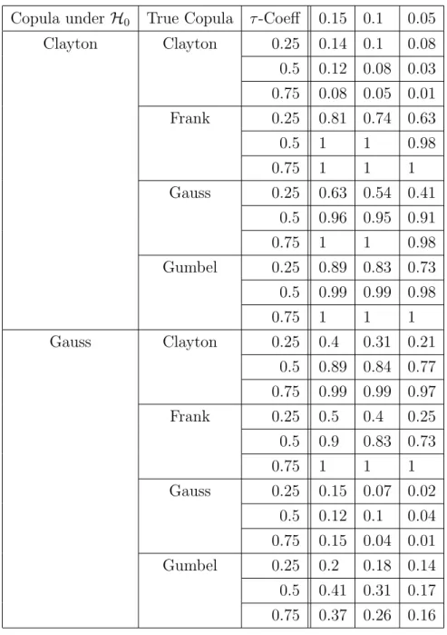
For our simulation study we use a similar setting as in Genest et. al. (2008). We choose a sample size of n = 150 and check the performance of the parametric bootstrap-procedure for two copula families, namely the Gauss- and the Clayton-Copula. The true copula is chosen from the Clayton-, Gauss-, Frank- or Gumbel-Family with parameter determined by the Kendall’s-τ-coefficient taking values in{0.25,0.5,0.75}. We useB = 100 Bootstrap-Replications and make 100 replications of the whole procedure in order to estimate the power of the test. Considering the parameters emerging in the definition of Tn we choose

ω = 1[0.25,0.975]

h = 0.7n−1/6

K(u, v) = (15/16)2₍₁₋_u2₎2₍₁₋_v2₎2₁

[−1,1]2(u, v)

The results are presented in Table 1. From this table it can be seen that the level of the test is well approximated in almost all cases, but there appears an effect of underestimation for larger

τ-coefficients.

Regarding the power of the test our results are quite comparable to other simulation studies considering the goodness-of-fit testing for copula families, see e.g. Genest et al. (2008). With stronger dependence, measured by the τ-coefficient, the test performs substantially better than in case of weak dependence. In comparison to the tests studied in Genest et al. (2008) it is remarkable that our bootstrap test outperforms all tests within that paper in case of the true copula family being Frank. In the other cases a comparison is more difficult. For example, if the copula under the null hypothesis is Gauss but the true copula is Gumbel, the L2_{-test proposed in this paper}

yields similar results as most of the tests investigated by Genest et. al. (2008), but there exist also more powerful tests. On the other hand, if the true copula is Clayton, the bootstrap version of

(19)

the test proposed by Fermanian (2005) yields a power comparable to the best tests investigated by Genest et. al. (2008). A similar observation can be made if the copula under the null hypothesis is Clayton. In this case the L2_{-test always yields a similar power as the best test considered by}

Genest. et.al. (2008).

For further conclusions and interpretations of the results, especially in comparison to other tests, we refer to the extensive simulation study in the paper of Genest et al. (2008).

6 Appendix

6.1 Proof of identity (3.30)

Using the notation

h∗ nm(Yi, Yk) := −1 h Z (dK)h(u−Yi)(1(Yk≤Yi)−Yi)∂θmτ(u, θ ∗ L2)ω(u)du (6.1)

(where ∂θm denotes the derivative with respect to the m-th component of the vector θ, for m =

1, . . . , q) we obtain the decomposition

An2m =A(1)n2m+A

(2)

n2m

(6.2)

for them-th component of the vectorAn2, where the random variablesAn(i2)m (i= 1,2) are defined

by A(1)_n₂_m = −1 n2_h n X i=1 Z (dK)_h(u−Yi)(1−Yi)∂θmτ(u, θ ∗ L2)ω(u)du, (6.3) A(2)_n₂_m = 1 n2 X k6=i h∗_nm(Yi, Yk). (6.4)

A straightforward standard calculation yields the estimate A(1)_n₂_m = oP(n−

1

2). The second term

A(2)_n₂_m can be identified as a non-degenerate U-statistic

A(2)_n₂_m = 1 n2 X i<j ˜ hnm= n−1 2n µ n 2 ¶₋₁ Un, (6.5)

where ˜hnm(Yi, Yk) = h∗nm(Yi, Yk) +h∗nm(Yk, Yi) denotes the symmetrized kernel of Un. A

straight-forward but tedious calculation yields the estimate E

h ˜ h2 nm(Yi, Yk) i =O(h−2_{) =} _o₍_n₎_, _{so that the}

assumptions of Lemma 3.1 in Zheng (1996) are fulfilled. This result gives ˜

A(2)_n₂_m−A_n(2)₂_m =oP(n−

1 2),

(6.6)

where ˜A(2)_n₂_mdenotes the orthogonal projection ˜A(2)_n₂_m = 1

n P_n i=1r˜nm(Yi) and ˜rnm(Yi) :=E h ˜ hnm(Yi, Yk)|Yi i . Finally, observing that E[h∗

nm(Yi, Yk)|Yi =yi] = 0, it follows that rnm(Yi) = ˜rnm(Yi) which yields

(20)

Copula under H0 True Copula τ-Coeff 0.15 0.1 0.05 Clayton Clayton 0.25 0.14 0.1 0.08 0.5 0.12 0.08 0.03 0.75 0.08 0.05 0.01 Frank 0.25 0.81 0.74 0.63 0.5 1 1 0.98 0.75 1 1 1 Gauss 0.25 0.63 0.54 0.41 0.5 0.96 0.95 0.91 0.75 1 1 0.98 Gumbel 0.25 0.89 0.83 0.73 0.5 0.99 0.99 0.98 0.75 1 1 1 Gauss Clayton 0.25 0.4 0.31 0.21 0.5 0.89 0.84 0.77 0.75 0.99 0.99 0.97 Frank 0.25 0.5 0.4 0.25 0.5 0.9 0.83 0.73 0.75 1 1 1 Gauss 0.25 0.15 0.07 0.02 0.5 0.12 0.1 0.04 0.75 0.15 0.04 0.01 Gumbel 0.25 0.2 0.18 0.14 0.5 0.41 0.31 0.17 0.75 0.37 0.26 0.16

Table 1: Simulated rejection probabilities of the L2_{-type test for various null hypotheses and}

alter-natives. The sample size is n= 150 and B = 100 parametric Bootstrap-replications have been

(21)

6.2 Proof of identity (4.10)

The proof of equation (4.10) follows along the same lines as the one given in appendix A via application of Lemma 3.1 in Zheng (1996). Using the notation ˜kn(Yi, Yk) := k∗n(Yi, Yk) +kn∗(Yk, Yi)

for the symmetrizied kernel we obtain the following identification of W_n(2₄,2) as a non-degenerate U-statistic: W_n(2₄,2) = 2 n2 X i<k ˜ kn(Yi, Yk) = n−1 n µ n 2 ¶₋₁ Un. (6.7)

A straightforward calculation shows E[˜k2

n(Yi, Yk)] = O(h−2) =o(n), and an application of Lemma

3.1 in Zheng (1996) yields c W_n(2₄,2)−W_n(2₄,2) =oP(n− 1 2), (6.8)

wherecW_n(2₄,2)denotes the orthogonal projectioncW_n(2₄,2) = 2

n

P_n

i=1s˜n(Yi) with ˜sn(Yi) = E[˜kn(Yi, Yk)|Yi].

Observing that E[k∗

n(Yi, Yk|Yi =yi] = 0 we obtain ˜sn(Yi) =sn(Yi) and the assertion follows.

6.3 Proof of identity (4.14)

By means of a Taylor expansion we obtain the decomposition

Wn6 =Wn(1)6 +W

(2)

n6 ,

(6.9)

where the random variables W_n(i₆) are defined by

W_n(1)₆ =−2 Z Kh(u−t)(τ0−τ∗)(t)Kh(u−s)∂θTτ(s, θM L∗ )(bθM L−θ∗M L)ω(u)dt ds du, W_n(2)₆ =− Z Kh(u−t)(τ0−τ∗)(t)Kh(u−s)(θbM L−θM L∗ )T∂θθ2 τ(s,θ˜) (θbM L−θM L∗ )ω(u)dt ds du,

for some ˜θ with kθ˜−θ∗

M Lk ≤ kθbM L−θM L∗ k. A straightforward calculation yields

W_n(2)₆ =OP µ° ° °bθM L−θM L∗ ° ° °2 ¶ =OP(n−1) = oP(n− 1 2).

Using identity (3.4) from Theorem 3.1 we obtain

W_n(1)₆ =−2 n n X i=1 Z Kh(u−t)(τ0−τ∗)(t)Kh(u−s)∂θTτ(s, θM L∗ )ω(u)du dt ds D(Yi) + oP µ 1 √ n ¶ .

Finally, considering expansions of (τ0 −τ∗) and ω, the dominating sum can be estimated by

−2

n

P_n

i=1βM LT D(Yi) +oP(n−

1

(22)

Acknowledgments. The authors would also like to thank M. Stein, who typed parts of this paper with considerable technical expertise. Financial support by the Deutsche Forschungsgemeinschaft (SFB 823, Statistik nichtlinearer dynamischer Prozesse) is gratefully acknowledged. The work of H. Dette was supported in part by a NIH grant award IR01GM072876:01A1.

References

Berger, J.O., Delampady, M. (1987). Testing precise hypotheses. Statist. Sci. 2, 317-335.

Bickel, P. and Rosenblatt, M. (1973). On some global measures of the deviations of density function estimators. Ann. Statist. 1, 1071-1095.

B¨ucher, A. (2008). Validation von Copula-Modellen. Diplomarbeit, Ruhr-Universit¨at Bochum, Germany.

Charpentier, A., Fermanian, J.-D. and Scaillet, O. (2007). The estimation of copulas: theory and practice. In Copulas: From theory to application in finance, edited by Rank, J., published by Risk Publications, London.

Cui, S. and Sun, Y. (2004). Checking for the gamma frailty distribution under the marginal proportional hazards frailty model. Statistica Sinica 14, 249-267.

Dobri´c, J. and Schmid, F. (2007). A goodness of fit test for copulas based on Rosenblatt’s trans-formation. Computational Statistics & Data Analysis 51, 4633-4642.

Embrechts, P., McNeil, A.J. and Straumann, D. (2002). Correlation and dependence in risk management: properties and pitfalls . In Risk management: value at risk and beyond, edited by Dempster M., published by Cambridge University Press, Cambridge.

Fan, Y. and Linton, O. (2003). Some higher order theory for a consistent nonparametric model specification test. Journal of Statistical Planning and Inference 109, no. 1-2, 125-154.

Fermanian, J.-D. (2005). Goodness-of-fit tests for copulas. Journal of Multivariate Analysis, 95, 119- 152.

Frees, E.W. and Valdez, E.A. (1998). Understanding relationships using copulas. North American Actuarial Journal 2, 1-25.

Genest, C. and Favre, A.-C. (2007). Everything you always wanted to know about copula modeling but were afraid to ask. Journal of Hydrologic Engineering 12, 347-368.

Genest C., Ghoudi, K. and Rivest, L.-P. (1995). A semiparametric estimation procedure of depen-dence parameters in multivariate families of distributions. Biometrika 82, 543-552.

Genest, C. and Rémillard, B. (2008). Validity of the parametric bootstrap for goodness-of-fit testing in semiparametric models. Annales de l’Institut Henri Poincaré. Probabilités et Statistiques 44 (in press).

(23)

Genest, C., R´emillard, B. and Beaudoin, D. (2008). Goodness-of-fit tests for copulas: A review and a power study. Insurance: Mathematics and Economics, 42, in press.

H¨ardle, W. and Mammen, E. (1993). Testing parametric versus nonparametric regression, Ann. Statist. 21, 1926-1947.

Hu, H.L. (1998). Large sample theory of pseudo-maximum likelihood estimates in semiparametric models. PhD Thesis, University of Washington, Department of Statistics, Seattle.

Joe, H. (1997). Multivariate Models and Dependence Concepts. Chapman & Hall, London. Klaassen, C.A.J. and Wellner, J.A. (1997). Efficient estimation in the bivariate normal copula model: normal margins are least favourable. Bernoulli 3, 55-77.

Malevergne, Y. and Sornette, D. (2003). Testing the Gaussian copula hypothesis for financial assets dependences. Quantitative Finance 3, 231-250.

McNeil, A.J., Frey, R. and Embrechts, P. (2005). Quantitative Risk Management. Princeton University Press, Princeton, N.J.

Nelson, R.B. (2006). An Introduction to Copulas, second ed. Springer, New York.

Scaillet, O. (2007). Kernel based goodness-of-fit tests for copulas with fixed smoothing parameters. Journal of Multivariate Analysis 98, 533-543.

Van der Vaart, A.W. (1998). Asymptotic Statistics. Cambridge Series in Statistical and Proba-bilistic Mathematics. Cambridge University Press, Cambridge.

Zheng, J.X. (1996). A consistent test of functional form via nonparametric estimation techniques. Journal of Econometrics 75, 263-289.

(24)

(25)

(26)