Variable Selection for Covariate Dependent Dirichlet
Process Mixtures of Regressions
William Barcella
∗1, Maria De Iorio
1and Gianluca Baio
11
Department of Statistical Science, University College London, London, UK
August 5, 2015
Abstract
Dirichlet Process Mixture (DPM) models have been increasingly employed to specify random partition models that take into account possible patterns within the covariates. Furthermore, in response to large numbers of covariates, methods for selecting the most important covariates have been proposed. Commonly, the covariates are chosen either for their importance in determining the clustering of the observations or for their effect on the level of a response variable (in case a regression model is specified). Typically both strategies involve the specification of latent indicators that regulate the inclusion of the covariates in the model. Common examples involve the use of spike and slab prior distributions. In this work we review the most relevant DPM models that include the covariate information in the induced partition of the observations and we focus extensively on available variable selection techniques for these models. We highlight the main features of each model and demonstrate them in simulations.
Keywords. Dirichlet Process Mixture models, random partition models, Bayesian variable selection, spike and slab distributions, model misspecification.
1
Introduction
Bayesian nonparametric literature has been increasingly focusing on models that can cluster observed units according to possible patterns in the covariates space. This mod-elling strategy is usually referred to as Random Partition Model with Covariates (RPMx,
Müller and Quintana[2010]) and has been successfully applied to a wide range of real-data problems, including epidemiology, survival analysis, genomics, pharmacokinetics.
Usually, an RPMx is constructed starting with a Dirichlet Process Mixture (DPM,
Antoniak [1974]) model. This is characterized by specifying a Dirichlet Process (DP,
Ferguson[1973]) prior on the parameters of the sampling model. The popularity of these models is due to fact that they allow for high flexibility and that the posterior distribu-tion of interests can be generally explored by efficient computadistribu-tional algorithms. DPM models induce a partition of the observations in clusters, with the probability of belong-ing to a specific cluster proportional to the cluster’s cardinality. This imposes a normal
behavior on the partition. Recently, a wealth of research has been focussing on compli-cating the clustering structure, by introducing dependence of the cluster probability on covariates. Moreover, RPMx have been extended to embed latent parameters with the aim of performing variable selection. The role of the latent variables in the RPMx frame-work consists primarily in identifying the subset of variables that are more discriminant in terms of the partition. The variable selection output is just the posterior distribu-tion of the latent indicators, which are commonly treated as any other model parameter and whose distribution is often approximated by Markov Chain Monte Carlo (MCMC) techniques.
The main objective of this paper is to review the most relevant RPMx models, defined through Dirichlet Process Mixtures. We dedicate particular attention to the available variable selection techniques. The rest of the work is organized as follows. In Section
2 we review the relevant theory about DPM models. In Section 3 we present RPMx models within a DPM framework, while in Section4we review available variable selection methods. Section 5 introduces an extension of RPMx models while in Section 6 we presents a simulation study. We conclude with a final discussion in Section 7.
2
Dirichlet Process Mixture Models
The Dirichlet Process (DP) is a distribution defined over a space of random distributions (Ferguson [1973]). A constructive definition is presented by Sethuraman [1991], who showed that if a random probability measure G is distributed according to a DP with parameters α∈R+ and base measure G
0 defined on the metric spaceΘ, then
G=
∞
X
k=1
ψkδθk (1)
where the elements θ1, θ2, . . . are iid realizations from G0, δθk is the Dirac measure that
assigns a unitary mass of probability in correspondence of location θk and the ψk are constructed following the stick breaking procedure (see Ishwaran and James [2001] for details): ψk =φk k−1 Y j=1 (1−φj), (2) with φk iid
∼ Beta(1, α). By construction 0 ≤ ψk ≤ 1 and
P∞
k=1ψk = 1. The resulting random measure G is defined on the same support of G0, i.e. Θ. A more compact
notation is G∼DP(α, G0)
Another common representation of the DP, which allows for efficient MCMC schemes, has been provided by Blackwell and MacQueen [1973]. Let us consider a sample of n
components θ = (θ1, . . . , θn) from a random distribution G. If G is distributed as a DP(α, G0), then by integrating out Gfrom the joint distribution of θ1, . . . , θn, we obtain the predictive prior distribution ofθi givenθ(i), which is the vector obtained by removing the i-th component from θ:
θi |θ(i) ∼ 1 α+n−1 X i06=i δθi0(θi) + α α+n−1G0(θi) (3)
Equation 3 is generally referred to as Blackwell-MacQueen urn. In particular, the first part of Equation 3 can be rewritten as Pk
the number of observations that have value equal to θj∗. The vector θ∗ = (θ1∗, . . . , θk∗) contains the unique values of the sequence θ(i). Since Equation 3 is a mixture of atoms,
there is a positive probability that k≤(n−1). This aspect is due to the discreetness of the DP samples (Blackwell [1973]): there is a positive probability of ties, i.e. that two random draws fromG∼DP(·,·)are identical. From Equation3it is also clear that there is a higher probability that a new (as yet unobserved) unit will be assigned to a more numerous cluster.
This aggregating property of DP makes it particularly effective to deal with clustering problem. In fact, arguably the most famous application of the DP is the Dirichlet Process Mixture (DPM) model (Antoniak [1974],Escobar and West [1995],Lo [1984]), a class of models that can be expressed hierarchically as follows:
y1, . . . , yn |θ1, . . . , θn ind ∼ p(yi |θi) θ1, . . . , θn|G iid ∼ G (4) G ∼ DP(α, G0)
This model assumes individual level parameters θi, for i = 1, . . . , n. The vector of pa-rameters will have some ties with probability greater than zero. This is because we set each one of them to have a distribution G which is a DP. This will have two main con-sequences: (i) the sequence θ = (θ1, . . . , θn) reduces to the sequence of its unique values
θ∗ = (θ∗1, . . . , θ∗k), with k ≤ n, (ii) the vector s= (s1, . . . , sn) with si ∈ {1, . . . , k}, which
associates each observation with a specific value among the components of the vectorθ∗, defines a partition of the observations.
An alternative representation of the DPM model is given by:
y1, . . . , yn |G iid ∼ p(y|G) p(y|G) = Z p(y|θ)G(dθ) (5) G ∼ DP(α, G0),
Recalling the discrete nature of the DP samples as well as its representation in Equation
1, we can rewrite the sampling model as a infinite mixture model:
y1, . . . , yn |G iid ∼ ∞ X k=1 ψkp(y |θk).
The vector s defines a partition because every subject i for i = 1, . . . , n cannot be associated simultaneously with more than one cluster. Letρndenote the partition of the
n observations implied bys. It is easy to prove that the prior distribution for ρninduced by the use of the DP prior is:
p(ρn) = αk α(n) k Y j=1 (nj −1)! (6)
where α(n) = α(α+ 1). . .(α+n −1) (take i in Equation 3 to be the last observation
for i = 1, . . . , n, exploiting the exchangeability of the Blackwell-MacQueen urn). This
defines an Exchangeable Partition Probability Function (EPPF, seePitman[1996]), where exchangeability arises from the fact that the partition does not depend on the labels of the observations or of the clusters, but only on the cardinality of the groups.
Therefore, a DPM model can be represented as a Random Partition Model (RPM, seeLau and Green[2007] for details) through p(ρn). An RPM is characterized by within-cluster-submodels and by a prior distribution on the partition. This is evident when writing the joint probability of the DPM in Equation 4 (Lo[1984]) as :
p(ρn,y,θ∗)∝ k Y j=1 Y i∈Sj p(yi |θ∗j)g0(θ∗j)α(nj−1)! (7)
whereg0 is the density associated with the distributionG0, whileSj ={i:si =j, for i=
1, . . . , n}. The termα(nj−1)!is calledcohesion functionfor thej-th group and is denoted
by c(Sj). Since p(ρn) can be seen as the product of the cohesion functions for each of the groups, this links the DPM with a specific type of RPM called Product Partition Model (PPM, Barry and Hartigan [1992], Hartigan [1990]), characterized in the same way. Using Equation 3, it is possible to specify the conditional posterior distribution of
θi for the model in Equation 7as follows:
p(θi |θ(i),y)∝ k X j=1 njp(yi |θj∗)δθj∗+α Z p(yi |θ)dG0(θ)g0(θ |yi). (8)
Particularly within a regression framework, recent Bayesian literature has focussed on defining RPM models allowing for covariates information when inferring the partition of the observations. This is usually obtained by modifying the cohesion function to account for covariates patterns. At the same time, there has been an increasing interest in performing variable selection within the context of RPM with covariates to identify the most informative variables for the partition. In the next sections we will first review the main methodologies for specifying DPM-based RPM with covariates and then we will present state of the art procedures for variable selection.
3
Covariate dependent DPM
Let us consider a matrix of covariatesX withn rows andD columns and letxi denote a row. In many applications, it is desirable to express a prior distribution on the partition that is a function of X, i.e. p(ρn |X), instead of letting the probability of the partition depending (a priori) only on the cardinality of the clusters. We call this type of models Random Partition Model with Covariates (RPMx).
We will focus on RPMx models that admit a DPM representation. To this end we allow the cohesion function to include the covariates, however, we assume that the overall probability of a partition is still specified as the product of cohesion functions of each cluster: p(ρn|X)∝ k Y j=1 c(Sj,Xjρ) (9)
where, for j = 1, . . . k, Xρj is the subset of the rows of X associated with cluster j. In the following sections we will review the most popular choices of covariate dependent cohesion functions.
In a regression framework, when the research interest is in modelling the relationship between a response variable y and a set of covariates X, i.e. studying the distribution of p(y | X,θ), the application of RPMx models has been very frequent. This is mainly
for two reasons. First, RPMx are flexible models, which allow to cluster the observations according to patterns within the covariates and then to specify a cluster-specific regression model. Secondly, they often lead to improved predictions: if we want to predict the response for a new subject with a specific set of covariates, then a RPMx model will assign higher probability that the new subject belongs to the cluster that contains the most similar covariates profile.
3.1
Augmented Response Models
The most common strategy to include information aboutX into the partition model in a DPM framework has been to treat each covariate as a random variable,i.e. by specifying a suitable probability model. Müller et al.[1996] were the first to introduce this idea within the DPM framework. In their work they consider an augmented model defined on Z = (y,X) and their objective is to estimate the smooth function g(X) = E(y | X). They approach the problem by modelling Z as a DPM of (D+R)-dimensional distributions, whereR is the dimension of the response variable (usually R= 1). LetΛ∗ be the matrix containing the unique parameters for thekclusters,(Λ∗1, . . . ,Λ∗k). Considering now a new observation z˜= (˜y,x)˜ , its predictive distribution can be derived as:
p(˜y,x˜|Λ∗)∝ k X j=1 njp(˜y,x˜|Λ∗j) +α Z p(˜y,x˜ |Λ)dG0(Λ)
In practice x˜ is known, but assuming uncertainty about its realized value allows us to rearrange the latter equation as
p(˜y|x˜,Λ∗)∝ k X j=1 njp(x˜|Λj∗)p(˜y|x˜,Λ ∗ j) +α Z p(˜y |x˜,Λ)p(x˜ |Λ)dG0(Λ)
using Bayes’ theorem. The quantity njp(x˜ | Λ∗j) depends on the cardinality of group j and on a measure of how likely it is that the new observation will be clustered in group
j, based on the value of its covariates. The latter is the likelihood of the observed x˜. The smooth function g(X) is then estimated by taking the expectation of p(˜y | x˜,Λ∗). Muller, Erkanli and West describe in details the case whereZ is a mixture of multivariate Gaussian distribution. This leads to easy calculations and to close form expression for
g(X).
A similar approach has been adopted by Müller et al. [2011]. They have originally proposed a modification of a PPM, the PPMx (PPM with covariates), to incorporate measures of similarity among the covariates within each cluster employing the following structure for the prior on the partition:
p(ρn|X)∝
k
Y
j=1
c(Sj)f(Xρj), (10)
where f(·), called similarity function, is an ad hoc function that takes large values for highly similar values of the covariates. The authors propose as a default choice for
f(·) a probability distribution. In this way f(Xρj) can be seen as the likelihood of the covariates belonging to cluster j, from which the cluster specific parameters have been
integrated out. Given the cluster specific parameters for the covariates, the auxiliary joint probability of a PPMx is:
f(y,X,θ∗,ζ∗1, . . . ,ζ∗D, ρn)∝ k Y j=1 Y i∈Sj p(yi |θ∗j,xi)f(xi |ζj∗1, . . . , ζ ∗ jD) p(θj∗)f(ζj∗)c(Sj) (11) whereθ∗ and ζ∗1, . . . ,ζ∗D represent the unique values of the parameters of the distribution of the response and of the covariates for the k clusters respectively. Equation 11 shows that the PPMx is a generalization of the methodology proposed in Müller et al. [1996]. Taking c(Sj) in Equation 11 to be the cohesion function implied by the DP and the covariates to be random variables with distribution p(xi | ζi1, . . . , ζiD) (thus allowing the similarity function to be a valid probability density for the covariates), the PPMx simply reduces to a DPM on the joint distribution of the response and the covariates representable by the following hierarchy:
y1, . . . , yn|X,θ ind ∼ p(yi |xi, θi) x1, . . . ,xn |ζ1, . . . ,ζn ind ∼ p(xi |ζi) (12) (θ1,ζ1), . . . ,(θn,ζn)|G iid ∼ G G ∼ DP(α, G0)
with G0 = G0θ×G0ζ, θ = (θ1, . . . , θn) and ζi = (ζi1, . . . , ζiD). Both Equation 11 and
12 define a PPMx, in which θ and ζ are assumed a priori independent. Therefore we conclude that every DPM can be represented as a PPMx, but the reverse is not always true. For this relation to hold, it is necessary thatp(yi,xi |θi,ζi) =p(yi |θi,xi)p(xi |ζi). In this perspective the PPMx generalizes the work by Müller et al. [1996] allowing for the possibility of user-specific models for the covariates (via the similarity function).
Alternatively,Park and Dunson[2010] have proposed a Generalized Product Partition Model (GPPM) to include information on the covariates in a PPM. The authors consider the covariates as generated by some probability distribution and first infer a PPM on the covariates only. Subsequently the posterior probability of the partition for the model on the covariates is used as prior probability for the partition of the response variable. This leads to the same joint model in Equation11under the assumption of independence between the parameters of the covariates and response models.
Within the PPMx framework in Equation 11, the sampling model p(yi | θ∗j,xi) does not necessarily need to be a linear regression. Hannah et al.[2011] have extended Equation
11 to the broader Generalized Linear Model (GLM) framework through the appropriate specification of p(yi | θ∗j,xi). This generalization allows the users to handle different types of data. They refer to this model as DP-GLM (see alsoShahbaba and Neal[2009]). A parametric version of the DP-GLM constitutes a particular case of the Hierarchical Mixture of Experts (HME) model introduced by Jordan and Jacobs[1994] and specified in a Bayesian framework by Bishop and Svenskn [2002].
An R package is available for the PPMx (https://www.ma.utexas.edu/users/pmueller/
prog.html#PPMx).
3.2
Profile Regression
Profile Regression (PR; Molitor et al. [2010]) offers an alternative strategy to account for covariate information when specifying the partition prior model. Molitor et al. [2010]
describe the case of a binary outcomey = (y1, . . . , yn)which is common in epidemiologic applications, but the model is easily generalized to different types of response variable. The PR model consists of two submodels. The first one is the model for the response:
yi |pi ∼Bernoulli(pi) with a logistic regression on the mean pi:
log pi 1−pi =θj∗+κwi,
wherewiis a set of confounding variables with coefficientsκwhileθ∗j is a random intercept depending on the cluster allocation for observation i, with si =j.
The second submodel is a mixture model on the covariates, such that conditioning on the cluster assignment vector, the probability of a specific covariate profile becomes:
xi |ζ∗1, . . . ,ζ
∗
D ∼p(xi |ζj∗1, . . . , ζ
∗
jD), (13)
where ζjd∗ is the element of ζ∗d corresponding to cluster j and to the d-th covariate. In order to consistently estimate the posterior distribution of the partition and the partition specific parameters, the authors propose to model jointly the random intercepts of the first submodel and the parameters of the covariates model in sub-model 13 ac-cording to a DP with parameter α and G0, with G0 being the product measure of G0θ and G0ζ. In this way the resulting partition is informed by the information within the covariates and the response.
This model can also be specified as an augmented response DPM model. Exploiting the relation between DPM and PPM and ignoring the confounding variables, we can rewrite the joint probability of the PR in a PPMx framework as follows:
p(y,X,θ∗,ζ∗1, . . . ,ζ∗D, ρn)∝ k Y j=1 Y i∈Sj p(yi |θj∗)p(xi |ζj∗1, . . . , ζ ∗ jD) p(θj∗)p(ζj∗1, . . . , ζjD∗ )c(Sj)
where the cohesion function in Equation11becomesc(Sj) =
Qk
j=1α(nj−1)!,p(θj∗) =g0θ
and p(ζj∗1, . . . , ζjD∗ ) =g0ζ. This construction obviously defines a DPM of distributions on
(y,X).
An R package for PR is available on CRAN (http://cran.r-project.org/web/
packages/PReMiuM/) and presented in Liverani et al.[2015].
3.3
Dependent Dirichlet Process
An alternative way to introduce covariate dependent clustering in the DPM is to allow the weights and/or the locations in the stick breaking construction of the DP in Equation
1to depend on covariates. In particular, a covariate dependent DPM can be represented in the following way:
Gx = ∞ X k=1 ψk(x)δθk (14) ψk(x) = φk(x) k−1 Y j=1 [1−φj(x)],
under the constraint that P∞
k=1ψk(x) = 1. ψk(·) is a function of the covariates. In this
context x represents a point in some covariate space X and φk(x) is a realization of a suitable Beta distribution. The model defined in Equation 14 is a particular case of the Dependent Dirichlet Process (DDP, MacEachern [1999]). Each Gx is still marginally a DP for each x. In its original formulation, the DDP model allows for both covariates dependent weights (as in Equation 14) as well as for covariates dependent locations. However, in terms of clustering, Equation 14 presents the most relevant construction. In this case the specification of a distribution for ψk(x) is central, as it determines the structure of the dependence between the covariates and the weights, and consequently the way the covariate profiles inform the clustering structure. Although assuming thatψk(x) are rescaled Beta random variables guarantees that theGx are marginally still a Dirichlet process (see, for example, the covariates order-based stick-breaking of Griffin and Steel
[2006]), several authors have preferred to use different models for φk(x)in order to allow for more flexible stick-breaking processes. Examples include the kernel stick-breaking in
Dunson and Park [2008], the probit stick-breaking in Chung and Dunson [2009] and in
Rodriguez and Dunson [2011] and the logistic stick-breaking in Ren et al. [2011] among the others.
The choice of the distribution for ψk(x) determines the DDP (or a dependent stick-breaking), which can then be used used as mixing measure in a hierarchical model:
p(yi |x,θ) =
∞
X
k=1
ψk(x)p(yi |θk)
Note that it is also possible to assume a regression model for y, p(yi | x, θk) instead of
p(yi |θk).
A related approach is the Weighed Mixture of DP (WMDP) by Dunson et al.[2007], which can be thought of as a finite mixture of DP distributed components, one for each covariate level. The weights of this mixture are specified as functions of the covariates. The resulting random measures maintain covariate independent locations and can be used conveniently to specify an infinite mixture model with covariates dependent weights.
3.4
Other Methods
In this section we briefly present two other methods that can be used to specify covariate dependent DPM.
The first is the Restricted DPM (RDPM) model introduced byWade et al.[2013]. The authors modify the usual structure of the DPM models by enforcing a strict dependence of the distribution of the partition on covariate proximity. This is achieved by restricting the probability measure on the partition implied by the DPM to satisfy an ordering rule for the covariates. The authors propose a covariate dependent probability distribution of the following form:
p(ρn |x) = αk α(n) n! k! k Y j=1 1 nj Isσx(1)≤...≤sσx(n),
wheresσx(1), . . . , sσx(n)is a permutation of the cluster assignment vector implied by, for
example, an increasing order of x1, . . . , xn when x is a one-dimensional covariate. It can be shown that this construction satisfies the Ewens sampling law (Ewens [1972]) for the probability on the cluster frequencies. This same law is satisfied by partitions implied by
Equation3. This class of models is appealing because it does not assume any distribution on the covariates when accounting for the covariate similarity. The authors show how to perform posterior inference in the RDPM through efficient MCMC algorithms. The mixing properties of the MCMC scheme are improved by restricting the parameter space of the cluster assignment to satisfy the covariate ordering condition.
A second alternative is represented by the Enriched Dirichlet Process Mixture (EDPM) model described in Wade et al. [2014]. The strength of this method consists in its abil-ity to create nested partitions (i.e. partitions within sets of a partition). To this end, the authors specify a DPM model for the response variable, setting a DP prior on the parameters of the sampling model for y. A DP prior dependent on the parameters of the response is used for the parameters of the probability model on the covariates. This construction leads to a nested clustering structure of the observations: a first level of clustering is at the response level, whereas a second level is obtained within the clusters formed at the first stage according to a DPM model on the covariates.
4
Covariate Dependent DPM and Variable Selection
Increasing research interest has been devoted to developing variable selection strategies in covariate dependent DPM models. Bayesian methods allow performing variable selection by specifying a prior on model space. See O’Hara et al. [2009] for a review of the main Bayesian variable selection strategies. In this section we will describe separately tools for augmented response models, Profile Regression and Dependent Dirichlet Process.
4.1
Variable Selection for Augmented Response Models
A variable selection strategy for the PPMx has been proposed byMüller et al.[2011] and described in details by Quintana et al. [2015]. Without loss of generality we start our discussion by considering the PPMx from the RPM point of view. It is possible to rewrite the similarity function in Equation 10 as the product of the similarity functions of each individual covariate,i.e. f(Xρj) =QD
d=1f(x
ρ
jd), wherex ρ
jd is the sub-vector of elements of columnd of X which include the elements corresponding to cluster j. Variable selection is then introduced employing binary indicatorsγjd∗ forj = 1, . . . kandd= 1, . . . , Dwithin the distribution of the partition:
p(ρn|X,γ)∝ k Y j=1 c(Sj) D Y d=1 f(xρjd)γ∗jd. (15)
The presence of the binary indicators allows the probability of the partition to depend on a subset of covariates within each cluster. In fact, γjd∗ = 0 eliminates the effect on the distribution of the partition of covariate d in cluster j. The model is completed by introducing in the hierarchy a prior distribution for the indicators. In particular, the authors propose to use Bernoulli prior distributions with the probability of success modeled using a logistic link.
Alternatively, Kunihama and Dunson [2014] consider an augmented response model and they propose a method for testing for conditional independence of the response and a specific covariate given all the other covariates. This involves the conditional mutual information for measuring the intensity of the dependence.
4.2
Variable Selection for PR
Papathomas et al. [2012] investigate the problem of performing variable selection within the Profile Regression framework when all the covariates are categorical (see also Pa-pathomas and Richardson [2014]). Let us recall that PR can be decomposed into two sub-models: a model on the covariates and one on the response. These are linked by using a joint DP prior on the set of parameters common to both the submodels. In order to introduce variable selection we need to rewrite Equation 13 in the following way:
xi |ζj∗1, . . . ζ ∗ jD ∼ D Y d=1 p(xid |ζjd∗).
Variable selection is then performed by replacing the distribution of each covariate with:
pVS(xid |ζjd∗ , πd) =πdp(xid |ζjd∗ ) + (1−πd)rd(xid), (16)
where the overscript VS indicates that the implied probability has been modified to perform variable selection, πd ∈ [0,1] is a continuos weight and rd(xid) indicates the proportion of times covariatedtakes value xid. From Equation 16it is evident that large values of πd indicate that covariate d is informative in terms of clustering.
The authors compared their approach that uses continuous weights to a version that employs cluster specific binary indicators for each covariate. This latter idea can be represented in the following way:
pBVS(xid |ζjd∗ ,γ ∗ d) =p(xid|ζjd∗ ) γjd∗ r d(xid)(1−γ ∗ jd),
where γjd∗ = 1 indicates that covariate d is informative with respect to cluster j. This approach is a generalization to Profile Regression of a solution proposed by Chung and Dunson [2009].
The results presented by Papathomas et al.[2012] show comparable performances of the two methods in terms of variable selection, although preference is given to continuos weights due to faster MCMC convergence.
An extension of the methods above has been proposed byLiverani et al. [2015] to deal with continuous covariates. This consists in modifying Equation 16 substituting rd(xid) with a suitable summary, for example the observed mean of the d-th covariate.
4.3
Variable Selection for DDP
To the best our knowledge, general variable selection strategies have not been imple-mented in the DDP framework. However, in the case of the dependent stick-breaking process Chung and Dunson [2009] show how to perform covariate selection when the weights of the random probability measure are constructed by a probit link stick-breaking. Thus, recalling the stick-breaking procedure in Equation14 the following specification is proposed: Gx = ∞ X k=1 ψk(x)δθk (17) ψk(x) = Φ (νk(x)) k−1 Y j=1 [1−Φ (νj(x))],
whereΦ(·)is the standard normal distribution and νk(·)is a linear predictor specified as
νk(x) =ξkx. Variable selection is then achieved by introducing binary indicators:
ξk ∼
D
Y
d=1
p(ξkd |ak)γkd(δ0(ξkd))(1−γkd), (18)
where ak denotes the cluster specific parameter of the distributions of ξkd for all d. The condition γkd = 0 prevents covariate d from having an effect on the k-th weight of Gx. Considering a regression sampling model p(yi | xi,θk), it is possible to link the results of the variable selection performed in Equation 18 directly to the parameters θkd in the regression model for the response so that when γkd = 0 both θkd and ξkd are set equal to 0.
5
Variable Selection for Covariate Dependent Dirichlet
Process Mixtures of Regressions
In section 4 we have presented the main contributions to variable selection for DPM models with covariate dependent partition structure. The methods described earlier allow us to find the most influential variables in terms of clustering properties. In this case, the research focus is not on the identification of covariates that have a high explanatory power on a response variables, as, for example, in regression settings where the primary interest is in modelling the relationship between a response y and a set of covariates.
Barcella et al.[2015] show how to perform variable selection in a regression framework when assuming an augmented response model. They assume a standard regression model, with a DPM prior on the regression coefficients. DPM prior distribution is specified on the covariates to allow for covariate dependent clustering. Variable selection is performed by specifying a spike and slab distribution (see George and McCulloch[1993] and Malsiner-Walli and Wagner [2011] for reviews) as base measure in the DP prior for the regression coefficients.
Spike and slab distributions are commonly used to perform variable selection in a regression framework and recently they have been used to this aim in DPM models. An example can be found inKim et al.[2009], who assume a linear regression sampling model with a DP prior on the regression coefficients with a spike and slab base measure of the following form: G0 = D Y d=1 (πdδ0(βd) + (1−πd)N(βd |µd, τd)). (19)
In this case the covariate are treated as fixed and we have a simple DPM of regression models. Employing a spike and slab base measure allows some coefficients in some cluster to be exactly equal zero, which is equivalent to performing variable selection within clusters. The main interest of the authors is to exploit this set-up in multiple hypothesis testing. A similar proposal can be found in Cai and Dunson [2005] for linear mixed models and inDunson et al.[2008] for binary regression (see alsoMacLehose and Dunson
[2010] and MacLehose et al.[2007]).
Building on the work of Kim et al. [2009], Barcella et al. [2015] assume that the co-variates are generated from some distribution. Then, they specify a joint DP prior on the regression coefficients and the parameters governing the distribution of the covariates,
assuming a priori independence between the two sets of parameters. Assuming a spike and slab base measure for the regression coefficients, this model allows to perform cluster specific variable selection, while, at the same time, the clustering structure is informed by both the covariate profiles and the relationship between response and covariates. The authors refer to this model as Random Partition Model with covariate Selection (RPMS). Note that inKim et al.[2009] the clustering structure is determined only by the relation-ship between response and explanatory variables.
5.1
RPMS: Model and Prior Specification
The RPMS can be generally represented by a hierarchy similar to the one in Equation
12. y|X,B, λ ∼ N(y |XBT, λIn) X |C ∼ n Y i=1 D Y d=1 Bernoulli(xid |ζid) (20) (β1,ζ1), . . . ,(βn,ζn)|G ∼ G G ∼ DP(α, G0),
whereB andC are matrices of parameters withnrows andDcolumns. βi fori= 1, ..., n
is a D-dimensional vector and is a row of B and ζi for i = 1, ..., n is a D-dimensional vector and is a row ofC. The RPMS in Equation20is designed in the original formulation to handle binary covariates, even though changing the specification of the distribution of the covariates enables us to include different type of variables. The base measure G0 has
the following form:
G0 =
D
Y
d=1
{[πdδ0(βd) + (1−πd)N(βd |µd, τd)]Beta(ζd|aζ, bζ)}, (21)
and we can rewrite G0 =G0β ×G0ζ. Following Kim et al. [2009], Barcella et al. use the
following prior distributions:
π1, . . . , πD |ω1, . . . , ωD ∼ D Y d=1 ((1−ωd)δ0(πd) +ωdBeta(πd |aπ, bπ)) ω1, . . . , ωD ∼ D Y d=1 Beta(ωd|aω, bω) (22) τ1, . . . , τD ∼ D Y d=1 Gamma(τd|aτ, bτ).
A similar structure for hyperpriors has been proposed by Lucas et al. [2006] to induce super-sparsity to the matrix of the regression coefficients. They further assume the same
λ for all the observations and λ ∼ Gamma(λ | aλ, bλ), while Kim et al. [2009] specify a DP prior on λ for extra flexibility. A Gamma(α | aα, bα) distribution is given to the precision parameter α of the DP process as suggested by Escobar and West [1995].
Posterior inference is performed through Markov Chain Monte Carlo (MCMC) tech-niques with Gibbs samplers (see Neal [2000]). A detailed description of the algorithm can be found in Barcella et al. [2015].
Variable selection output can be summarized in various ways. We describe here two possible alternatives. The first and more natural way is through exploring the posterior distribution of the regression coefficients for a given profile of covariates. Alternatively, fixing a convenient partition of the observations among those explored by the MCMC permits to sample from the posterior of the regression coefficients within each cluster.
The RPMS model is a DPM model on the joint distribution of(y,X). Similarly to the approach ofPark and Dunson [2010], it is possible to express the predictive (conditional) prior of the parameters for subjectiusing a modified Blackwell-MacQueen urn (Blackwell and MacQueen[1973]), which includes information on the covariates as follows:
(βi,ζi)|B(i),C(i),xi ∼q0(xi)G0(βi,ζi |xi) + k X j=1 njqj(xi)(δβ∗j ×δζ∗j), (23) where q0(xi) = qα˜ D Y d=1 Z p(xid |ζ)dG0ζ qj(xi) = q˜ D Y d=1 p(xid|ζjd∗ )
B and C are matrices whose rows are respectively β1, . . . ,βn and ζ1, . . . ,ζn (the super-script(i)indicates that thei-th row has been removed),kis the number of unique rows in the matrix [B(i),C(i)], obtained by binding column-wise the two matrices of parameters, ˜
q is a normalizing constant and we denote with × the product operation for measures. The derivation of Equation 23 is presented in the appendix of the work by Park and Dunson [2010].
The process defined in Equation 23 is useful to compute the predictive distribution of the response variable when a new set of covariates becomes available. In fact, it turns out that the predictive posterior distribution for y˜, given its covariates x˜ is
p(˜y|y,X,x) =˜
Z
p(˜y|y,X,x˜,β,ζ)dp(β,ζ |X,y,x)˜ (24)
and it can be computed numerically integrating G out of the joint probability model using Equation 23and integrating β and ζ through MCMC.
Moreover, from Equation 23 we can deduce that the prior probability for the i-th observation to be in an occupied cluster, say the j-th, is the cluster probability implied by the DP enriched by the marginal likelihood for the i-th row of the covariates. This has the effect of encouraging observations with similar covariate profiles to be assigned to the same cluster a priori.
We now need to define a measure of similarity between covariates. In the RPMS two covariates are similar if they share the same generating distribution. This is a sensible choice in the case of binary covariates because it encourages two observations to co-cluster when, for example, they have the same probability of having the same covariate taking value 1. When the covariates are continuos, it could be preferable to cluster the observations by specifying a distance between covariates and define the covariate proximity (instead of the likelihood similarity). An example is given by the Restricted DPM (Wade et al. [2013]).
The RPMS can also be described as a special case of PPMx. This is because the regression coefficients and the parameters corresponding to the covariate distribution are a priori independent. This becomes evident when considering the joint probability model:
p(ρn,y,X,B∗,C∗) = k Y j=1 Y i∈Sj p(yi |β∗j,xi)p(xi |ζ∗j) g0β(β∗j)g0ζ(ζ∗j)c(Sj), (25)
where B∗ and C∗ are the matrices with the unique rows β∗j and ζ∗j respectively and
c(Sj) is the DP cohesion function. g0β and g0ζ are the density of the distributions G0β and G0ζ. Equation 25also highlights the most important difference between the RPMS and the models similar to the one defined in Kim et al. [2009], where a spike and slab distribution is specified as base measure of the DP to perform variable selection, but there is no probability model on the covariates.
Proposition 5.1. Consider the model defined inKim et al. [2009] with DP base measure
G0 given in Equation 19. Consider also a unidimensional covariate. Then the cluster characterized by the value β = 0 suffers a priori of an inflated preferential attachment for any new observation. In particular, if an observation i is associated with βi = 0 then
the probability that the observation i0 co-clusters is:
p(βi0 =βi |βi = 0) =
1 +αω
α+ 1 . (26)
This result can be extended for multidimensional covariates considering the vector βi such that βi1 =. . .=βiD = 0.
Proof. See Appendix A
The RPMS does not suffer of the same drawback even in the case ofG0β being atomic at zero (a spike and slab distribution), as long as G0ζ is non-atomic. In fact, considering two draws from G0 = G0β ×G0ζ, say (β1, ζ1) and (β2, ζ2) and assuming D = 1 without
loss of generality, Pr ((β1, ζ1) = (β2, ζ2)) = 0 because, even if Pr(β1 = β2) 6= 0 (that is
when they are both equal to 0), Pr(ζ1 =ζ2) = 0.
6
Simulation Study
Assuming that the covariates are random and specifying an augmented probability model has the advantage of making posterior inference robust to model misspecification. We illustrate this point with two simulation studies in which we compare the results of the RPMS model with the model described in Kim et al. [2009], which, for simplicity, we refer to as Spike and Slab Model (SSM). Furthermore, we present also the performances of the Profile Regression (PR) and of its variable regression.
RPMS and SSM have the same hierarchical structure, except for the model for the covariates. In what follows, we only consider categorical covariates and we choose the same hyperparameters for both the models: aπ = 1, bπ = 0.15, aω = 1, bω = 0.15, aτ =
bτ = 1, aλ = bλ = 1, aα = bα = 1 and, only for the RPMS, aζ = bζ = 1. We do not update the parameter µd and we fix it equal to 0 for all d. As mentioned above, in both cases posterior inference is performed through MCMC algorithms. We initialize the algorithm starting with one cluster and fixing the regression coefficients equal to zero and the parameters for the covariates equal to 0.5 (this last specification is required only for
the RPMS). We run 15000 iterations, discarding the first 5000 as burn in. The PR has been initialized with the default values of the R package PReMiuM and 10000 samples have been saved after discarding the first 5000. A Normal model for the response and a Bernoulli model for the covariates have been assumed. Confounding variables have been ignored. We focus exclusively on the variable selection via continuous indicators (see Equation 16) following the suggestion of the authors.
6.1
Scenario 1
We simulate a dataset with n = 200 observations. We consider two binary covariates,
D= 2, and each entryxid of the design matrix is generated from a Bernoulli distribution with mean equal to0.5. The responseyiis generated fromN(xi1β¯i1+xi2β¯i2+xi1xi2β¯i3,1),
where β¯i1 and β¯i2 denote the true value used to simulate the data. We generate two
clusters of observations of equal size, S1 and S2, withn1 =n2 = 100, by setting: β¯
∗
si=1 =
(3,5,9) in cluster 1 andβ¯∗s
i=2 = (0,5,0) in cluster 2.
The data generating process contains an interaction term only in one of the clusters (β¯i3 = 9). When fitting both the RPMS and the SSM, we intentionally do not specify
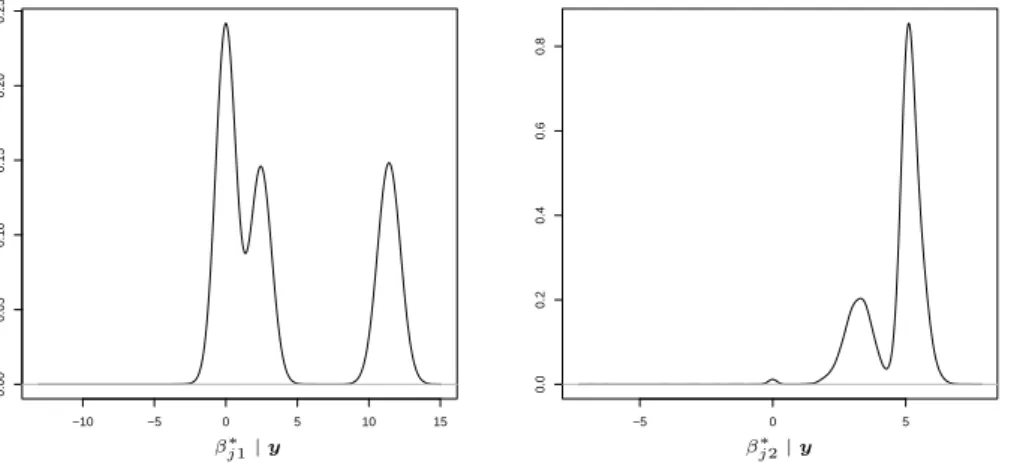
in-teraction terms in the regression sampling model. However the ability to perform variable selection jointly with covariate dependent clustering enables the RPMS to achieve robust predictive inference. To illustrate this property, let us consider the posterior distribution of the regression coefficients obtained by the SSM and the RPMS respectively. Given that the cluster allocation of the SSM depends only on the cardinality of the clusters, the posterior of the regression coefficients under this model is invariant with respect to the different patterns in the covariate vector. Figure1presents the posterior distribution for the regression coefficients of the two covariates under the SSM. In the RPMS, since
−10 −5 0 5 10 15 0.00 0.05 0.10 0.15 0.20 0.25 −5 0 5 0.0 0.2 0.4 0.6 0.8 βj∗1|y βj∗2|y
Figure 1: Posterior distribution ofβj∗1 (left) and ofβj∗2 (right) in scenario 1 for SSM. cluster allocation depends also on patterns in the covariate space, the distribution of the regression coefficients varies across different combinations of covariates. In our example there can be four different combinations: x˜1 = ˜x2 = 0, x˜1 = ˜x2 = 1, x˜1 = 1∧x˜2 = 0
and x1˜ = 0∧x2˜ = 1. In Figure 2 we show the posterior distribution of the regression coefficients obtained from RPMS, conditional on each of the four different covariates com-binations. The fact that in RPMS the cluster assignment, and consequently the posterior distribution of the coefficients, depends on the covariates allows us to detect the effect
−5 0 5 10 0 1 2 3 4 0 5 10 0.0 0.2 0.4 0.6 0.8 0 5 10 0.0 0.2 0.4 0.6 0.8 1.0 −5 0 5 10 15 0 1 2 3 βj∗1 βj∗1|x˜1= 0,˜x2= 0,y βj∗1|˜x1= 1,x˜2= 1,y βj∗1|x˜1= 1,˜x2= 0,y βj∗1|˜x1= 0,x˜2= 1,y −20 0 20 40 0 2 4 6 8 −20 −10 0 10 0.00 0.05 0.10 0.15 0.20 0.25 0.30 −40 −30 −20 −10 0 10 20 0.00 0.05 0.10 0.15 0.20 0.25 −10 −5 0 5 10 15 20 25 0 1 2 3 4 5 βj∗2 βj∗2|x˜1= 0,˜x2= 0,y βj∗2|˜x1= 1,x˜2= 1,y βj∗2|x˜1= 1,˜x2= 0,y βj∗2|˜x1= 0,x˜2= 1,y
Figure 2: Posterior distribution of βj∗1 (top) and of βj∗2 (bottom) considering the four possible combinations x˜1 = ˜x2 = 0, x˜1 = ˜x2 = 1, x˜1 = 1∧x˜2 = 0and x˜1 = 0∧x˜2 = 1in
scenario 1 for RPMS.
due to the interaction term by inferring a cluster in which it is more likely to find both the covariates equal to one and then estimating the cluster specific regression parameters. On the other hand, the SSM accounts for the interaction by estimating an extra component in the mixture model defined for the regression coefficients (see the left density in Figure
1).
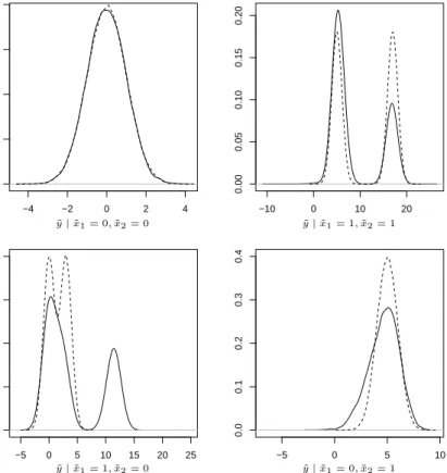
Obviously, this difference has a direct effect on the predictive distribution of the re-sponse. In Figure3we display the predictive distribution for the four combinations of the covariates obtained when fitting the SSM. As the covariates do not inform the partition,
−4 −2 0 2 4 0.0 0.1 0.2 0.3 0.4 −10 0 10 20 0.00 0.05 0.10 0.15 0.20 −5 0 5 10 15 20 25 0.00 0.05 0.10 0.15 0.20 −5 0 5 10 0.0 0.1 0.2 0.3 0.4 ˜ y|x˜1= 0,˜x2= 0 y˜|x˜1= 1,˜x2= 1 ˜ y|x˜1= 1,˜x2= 0 y˜|x˜1= 0,˜x2= 1
Figure 3: Predictive distribution of y for the four possible combinations x˜1 = ˜x2 = 0, ˜
x1 = ˜x2 = 1, x˜1 = 1∧x˜2 = 0 and x˜1 = 0∧x˜2 = 1 in scenario 1 obtained fitting the
SSM. The dashed line indicates the true density of the response for the four covariate combinations.
the posterior distribution of the regression coefficients displays an extra component in the mixture for each of the two regression parameters to accommodate for the interaction effect. This introduces a bias in the estimate of the predictive distribution in all the cases where at least one covariate is different from zero. This becomes more evident in the predictive distribution forx˜1 = 1 and x˜2 = 0.
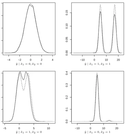
Figure 4 shows the predictive distributions obtained when fitting the RPMS. This example highlights how covariate dependent clustering protects from model misspecifica-tion, as it is evident from the top right panel in Figures 3 and 4 corresponding to both covariates equal to 1.
We finally present the performances of the PR in this first scenario. It is worth noticing that the PR leads to robust predictive inference thanks to the model on the covariates. The latter permits to identify the four combinations of the covariates and then associates to each of them a cluster specific mean in the response submodel. Consequently, PR identifies also the particular combinations of covariates that activates the interaction effect in one cluster. The results are presented in Figure 5
Figure 6 displays the continuous indicators employed by PR for performing variable selection. These highlight that both covariates are important in terms of determining the
−4 −2 0 2 4 0.0 0.1 0.2 0.3 0.4 −10 0 10 20 0.00 0.05 0.10 0.15 −5 0 5 10 0.00 0.05 0.10 0.15 0.20 −10 0 10 20 0.0 0.1 0.2 0.3 0.4 ˜ y|x˜1= 0,˜x2= 0 y˜|x˜1= 1,˜x2= 1 ˜ y|x˜1= 1,˜x2= 0 y˜|x˜1= 0,˜x2= 1
Figure 4: Predictive distribution of y for the four possible covariate combinations x˜1 = ˜
x2 = 0, x˜1 = ˜x2 = 1, x˜1 = 1∧x˜2 = 0 andx˜1 = 0∧x˜2 = 1 in scenario 1 under the RPMS.
The dashed line denotes the true density for y for the four covariate combinations. clustering structure. This is because the PR identifies clusters of response values sharing the same mean and the same combination of covariates, compensating in this way the model misspecification (note that in PR we are not regressing the response vector on the covariate matrix).
We conclude highlighting that we have not included an intercept neither for RPMS nor for SSM and, accordingly, we have generated the observations from a regression model that does not include the intercept. This has been done to facilitate the presentation of the results. We have also performed the same simulation of scenario 1 adding the intercept to RPMS and SSM and using observations generated from a regression model including cluster-specific intercepts and we have obtained equivalent results to those presented above.
6.2
Scenario 2
For the second simulation study we consider n = 200 observations and we assign them to 4 clusters, so that n1 = n2 =n3 =n4 = 50. We generate the response values from a
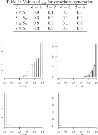
Normal distribution with cluster specific mean and unit precision. In particular, in the first cluster we assume the mean to be equal 5, while in the second cluster equal to -5, in the third cluster equal to 2 and in the forth cluster equal to 8. We also generate a matrix of covariates with D = 4 reflecting the clustering structure above. In particular, each covariate value is generated from a Bernoulli distribution with parameterζ¯id. The values of ζ¯id for each cluster are given in Table 1. In this scenario we include cluster-specific
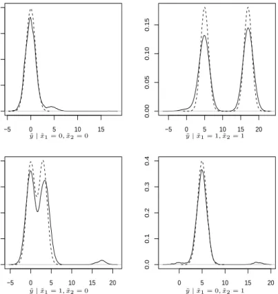
−5 0 5 10 15 0.0 0.1 0.2 0.3 0.4 N = 9000 Bandwidth = 0.1679 −5 0 5 10 15 20 0.00 0.05 0.10 0.15 N = 9000 Bandwidth = 0.9167 Density −5 0 5 10 15 20 0.00 0.05 0.10 0.15 0.20 0 5 10 15 20 0.0 0.1 0.2 0.3 0.4 Density ˜ y|x˜1= 0,x˜2= 0 y˜|˜x1= 1,x˜2= 1 ˜ y|x1˜ = 1,x2˜ = 0 y˜|˜x1= 0,x2˜ = 1
Figure 5: Predictive distribution of y for the four possible covariate combinations x1˜ = ˜
x2 = 0, x˜1 = ˜x2 = 1, x˜1 = 1∧x˜2 = 0 and x˜1 = 0∧x˜2 = 1 in scenario 1 under the PR.
The dashed line denotes the true density for y for the four covariate combinations.
0.0 0.2 0.4 0.6 0.8 1.0 0 5 10 15 20 25 30 0.0 0.2 0.4 0.6 0.8 1.0 0 20 40 60 80 100 π1|y π2|y
Figure 6: Posterior distribution of the continuous indicatorsπ1 andπ2 for PR in scenario 1. Values skewed toward 1 indicate the importance of the covariates for the clustering. intercepts for both RPMS and SSM.
The covariates contribute to determine the clustering structure and the PR is able to identify the covariates that are discriminant in terms of clustering. This is confirmed by Figure 7, where the posterior of the continuous indicators for the variable selection are skewed towards 1 for the first and the second covariate, and towards 0 for the third and the fourth covariate. This indicates that the last two covariates do not bring any clustering information.
Similarly to Scenario 1, the combinations of activated covariates are not distributed uniformly across the clusters. For example, the profile x˜ = (0,1,0,1) is more likely
Table 1: Values ofζ¯id for covariates generation. ¯ ζid d= 1 d= 2 d= 3 d= 4 i∈S1 0.9 0.1 0.1 0.9 i∈S2 0.3 0.9 0.1 0.9 i∈S3 0.8 0.3 0.1 0.9 i∈S4 0.3 0.9 0.1 0.9 0.0 0.2 0.4 0.6 0.8 1.0 0 1 2 3 4 5 0.0 0.2 0.4 0.6 0.8 1.0 0 5 10 15 0.0 0.2 0.4 0.6 0.8 1.0 0 5 10 15 0.0 0.2 0.4 0.6 0.8 1.0 0 10 20 30 40 π1|y π2|y π3|y π4|y
Figure 7: Posterior distribution of the continuous indicators π1, π2, π3 and π4 for PR
in scenario 2. Values skewed toward 1 indicate the importance of the covariates for the clustering.
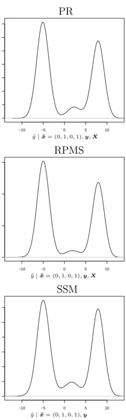
to be observed in clusters S2 and S4. As a consequence, under the PR the predictive
distribution for this profile of covariates should be dominated by the Normal components with mean -5 and 8, i.e. the cluster specific means corresponding to the second and the fourth cluster. This is confirmed by the top panel in Figure 8.
The same figure depicts also the predictive distributions for the RPMS (middle panel) and SSM (bottom panel) for the same combination of the covariates. Both distributions show clearly the two components centered on the values -5 and 8 (and also a third component with lower probability with mean 2). These distributions reflect the one obtained by PR, but both RPMS and SSM reach this result in different ways.
RPMS uses the spike and slab prior distribution for the regression coefficients within each cluster to set the coefficients for all for the covariates equal to 0, except the cluster-specific intercept which is modeled jointly with the parameters of the covariates model. In this way RPMS becomes equivalent to PR. This conclusion is also supported by looking at the posterior distribution of the partition of the observations which can be investigated using the posterior probabilities of co-clustering for all pairs of observations. These prob-abilities highlight the four groups of observations used for generating the observations. This result is equivalent to the one that we have obtained analyzing the clustering under
−10 −5 0 5 10 0.00 0.02 0.04 0.06 0.08 0.10 0.12 0.14 PR ˜ y|x˜= (0,1,0,1),y,X −10 −5 0 5 10 0.00 0.05 0.10 0.15 RPMS ˜ y|x˜= (0,1,0,1),y,X −10 −5 0 5 10 0.00 0.02 0.04 0.06 0.08 0.10 0.12 SSM ˜ y|x˜= (0,1,0,1),y
Figure 8: Predictive distribution of y for the combination of covariates x˜= (0,1,0,1)in scenario 2 for PR, RPMS and SSM (from the top).
PR. The robustness of the predictions using RPMS has been verified also for the other possible combinations of the covariates.
Also SSM achieves robust predictions for the combination x˜ = (0,1,0,1). This result can be explained looking at the posterior distribution of the regression coefficients. The posterior distribution of the intercept captures the levels of the response when the covari-ates are all equal to 0. The posterior distribution of the first regression coefficient adjust the posterior distribution of the intercept in order to identify the level of the response in the first and third cluster. This happens because the first covariate is often equal to 1 in these two clusters and rarely in the others. The posterior distribution of the second regression coefficient works as the first regression coefficient but for the second and fourth cluster. Finally, the posterior distributions of the last two coefficients shrink toward zero, since the respective covariates do not contain any information in terms of clustering. For
these reasons SSM leads to the correct predictive distribution for all combinations of the covariates. However, the posterior distribution of the partition of the observations explores more configurations compared to RPMS because SSM uses less information to estimate the clustering structure of the observations. Consequently, SSM identifies less clearly the four clusters from which the data are generated.
7
Discussion
In this paper we have reviewed the most relevant literature on Dirichlet Process Mixture models with covariate dependent weights and the corresponding techniques for variables selection. Covariates can offer extra information on the partition of the data and account-ing for possible structure within the covariates can improve the predictive performance of the model.
The most common solution to account for the presence of covariates within a DPM models consists of assuming the covariates as generated by a probability distribution and therefore specifying a joint DPM model on the augmented space including both response and explanatory variables. This solution is convenient in applications, as it becomes straightforward to obtain covariate dependent weights in the DPM model. This formulation has many advantages. In particular, it leads to improved predictions in regression setups, still allowing for efficient computations. The major drawback of this approach is related to the fact that considering a joint probability model for response and covariates may lead to the likelihood being dominated by the covariate specific terms, a problem that becomes particularly non-ignorable when dealing with a large number of covariates. A solution to this problem is represented by the EDPM model (Wade et al.
[2014]). This model introduces two clustering steps: first the observations are clustered on the basis of the response values and subsequently the model accounts for the covariate patterns within each of the clusters of the response.
Alternative solutions can be found in the literature on covariate dependent Random Partition Models, in particular in research concerning the Dependent Dirichlet Process and dependent stick-breaking process in general. These techniques offer an elegant way to account for the dependence of the weights in the stick-breaking representation on covariate information. However, when dealing with continuous covariates (or categorical with a large number of levels), these methods estimate a sequence of probabilities of belonging to the clusters for each observed level of the covariates, leading to difficulties in the interpretation of the clustering output. Moreover, posterior computations are often challenging when Gx is not marginally a DP, forcing the user to employ parametric approximations or expensive algorithms.
The variable selection techniques proposed in the literature for covariate dependent RPMs aim at identifying the most influential covariate for the partition of the observa-tions. Especially for the augmented response models (and consequently also for Profile Regression), the likelihood of the model of the covariates can dominate the DPM when a large number of covariates is involved. By introducing latent variables we can eliminate the effect of specific covariates in determining the partition and consequently mitigate this problem.
In many applications it is of interest to identify those covariates that best explain a response variable. The RPMS model extends the augmented response models to allow for variable selection in regression settings by specifying a spike and slab distributions
as base measures. Spike and slabs priors are commonly used in the Bayesian paradigm to perform variable selection and recently they have been employed in non-parametric settings in context of DPM of regressions. We have shown through simulations that spec-ifying a model on the covariates leads to inference which is robust to misspecification in the sampling distribution of the response. Of course, this comes at a computational cost. We have compared the performance of the RPMS with the SSM, a similar model where the covariates are considered fixed and not random. We have also presented re-sults achieved using the PR. In the RPMS cluster assignment depends also on covariate information, while in the SSM it is affected only by the response values. This difference is reflected in the posterior distribution of the regression coefficients, which is dependent on the particular pattern in the covariates when fitting a RPMS. Obviously, predictive inference under the RPMS is specific to the particular vector of covariates of a hypothet-ical new patient, while under the SSM the predictive distribution for a new individual is independent of his/her covariate profile. Also PR is robust to model misspecification, thanks to the model on the covariates. Finally, we have also highlighted the different concept of variable selection employed by PR and RPMS (or SSM equivalently).
We would like to conclude this review by pointing out that this is still a very open line of research and our main aim is to illustrate the most relevant contributions to date.
A
Proof Proposition 5.1
Let us consider for simplicity i = 1and i0 = 2. Employing the Blackwell-MacQueen urn (Equation3), fori= 1,β1 is drawn from the base measureG0with probability 1. So there
is some positive probability that it will take value equal to 0 due to the atomic structure of G0. Rewriting the conditional prior of β2 | (β1 = 0)as a Blackwell-MacQueen urn we
have that: β2 |(β1 = 0)∼ α α+ 1G0+ 1 α+ 1δ(β1=0)(β2) = = α α+ 1(ωδ0(β) + (1−ω)G0β) + 1 α+ 1δ(β1=0)(β2) = = α(1−ω) α+ 1 G0β + 1 +αω α+ 1 δ(β1=0)(β2)
Thus the probabilityp(β2 =β1 |β1 = 0) = 1+α+1αω, instead of the co-clustering probability
typical of the DP prior, which is equal to α1+1 (Antoniak [1974]). The exchangeability of the Dirichlet Process ensures that this is valid for any i6=i0.
References
Antoniak, C. E. (1974). Mixtures of dirichlet processes with applications to bayesian nonparametric problems. The annals of statistics, pages 1152–1174.
Barcella, W., De Iorio, M., Baio, G., and Malone-Lee, J. (2015). Variable selection in covariate dependent random partition models: an application to urinary tract infection.
arXiv preprint arXiv:1501.03537.
Barry, D. and Hartigan, J. A. (1992). Product partition models for change point problems.
Bishop, C. M. and Svenskn, M. (2002). Bayesian hierarchical mixtures of experts. In
Proceedings of the Nineteenth conference on Uncertainty in Artificial Intelligence, pages 57–64. Morgan Kaufmann Publishers Inc.
Blackwell, D. (1973). Discreteness of ferguson selections. The Annals of Statistics, 1(2):356–358.
Blackwell, D. and MacQueen, J. B. (1973). Ferguson distributions via pólya urn schemes.
The annals of statistics, pages 353–355.
Cai, B. and Dunson, D. B. (2005). Variable selection in nonparametric random effects models. Technical report, Department of Statistical Science, Duke University.
Chung, Y. and Dunson, D. B. (2009). Nonparametric bayes conditional distribution mod-eling with variable selection.Journal of the American Statistical Association, 104(488). Dunson, D. B., Herring, A. H., and Engel, S. M. (2008). Bayesian selection and clustering of polymorphisms in functionally related genes. Journal of the American Statistical Association, 103(482).
Dunson, D. B. and Park, J.-H. (2008). Kernel stick-breaking processes. Biometrika, 95(2):307–323.
Dunson, D. B., Pillai, N., and Park, J.-H. (2007). Bayesian density regression. Journal of the Royal Statistical Society: Series B (Statistical Methodology), 69(2):163–183. Escobar, M. D. and West, M. (1995). Bayesian density estimation and inference using
mixtures. Journal of the american statistical association, 90(430):577–588.
Ewens, W. J. (1972). The sampling theory of selectively neutral alleles. Theoretical population biology, 3(1):87–112.
Ferguson, T. S. (1973). A bayesian analysis of some nonparametric problems. The annals of statistics, pages 209–230.
George, E. I. and McCulloch, R. E. (1993). Variable selection via gibbs sampling. Journal of the American Statistical Association, 88(423):881–889.
Griffin, J. E. and Steel, M. J. (2006). Order-based dependent dirichlet processes. Journal of the American statistical Association, 101(473):179–194.
Hannah, L., Blei, D., and Powell, W. (2011). Dirichlet process mixtures of generalized linear models. Journal of Machine Learning Research, 1:1–33.
Hartigan, J. A. (1990). Partition models. Communications in Statistics-Theory and Methods, 19(8):2745–2756.
Ishwaran, H. and James, L. F. (2001). Gibbs sampling methods for stick-breaking priors.
Journal of the American Statistical Association, 96(453).
Jordan, M. I. and Jacobs, R. A. (1994). Hierarchical mixtures of experts and the em algorithm. Neural computation, 6(2):181–214.
Kim, S., Dahl, D. B., and Vannucci, M. (2009). Spiked dirichlet process prior for bayesian multiple hypothesis testing in random effects models. Bayesian analysis (Online), 4(4):707.
Kunihama, T. and Dunson, D. B. (2014). Nonparametric bayes inference on conditional independence. arXiv preprint arXiv:1404.1429.
Lau, J. W. and Green, P. J. (2007). Bayesian model-based clustering procedures. Journal of Computational and Graphical Statistics, 16(3):526–558.
Liverani, S., Hastie, D. I., Papathomas, M., and Richardson, S. (2015). Premium: an r package for profile regression mixture models using dirichlet processes. Journal of Statistical Software, 64(7).
Lo, A. Y. (1984). On a class of bayesian nonparametric estimates: I. density estimates.
The annals of statistics, 12(1):351–357.
Lucas, J., Carvalho, C., Wang, Q., Bild, A., Nevins, J., and West, M. (2006). Sparse sta-tistical modelling in gene expression genomics.Bayesian Inference for Gene Expression and Proteomics, 1.
MacEachern, S. N. (1999). Dependent nonparametric processes. In ASA proceedings of the section on Bayesian statistical science, pages 50–55.
MacLehose, R. F. and Dunson, D. B. (2010). Bayesian semiparametric multiple shrinkage.
Biometrics, 66(2):455–462.
MacLehose, R. F., Dunson, D. B., Herring, A. H., and Hoppin, J. A. (2007). Bayesian methods for highly correlated exposure data. Epidemiology, 18(2):199–207.
Malsiner-Walli, G. and Wagner, H. (2011). Comparing spike and slab priors for bayesian variable selection. Austrian Journal of Statistics, 40(4):241–264.
Molitor, J., Papathomas, M., Jerrett, M., and Richardson, S. (2010). Bayesian profile regression with an application to the national survey of children’s health. Biostatistics, page kxq013.
Müller, P., Erkanli, A., and West, M. (1996). Bayesian curve fitting using multivariate normal mixtures. Biometrika, 83(1):67–79.
Müller, P. and Quintana, F. (2010). Random partition models with regression on covari-ates. Journal of statistical planning and inference, 140(10):2801–2808.
Müller, P., Quintana, F., and Rosner, G. L. (2011). A product partition model with regression on covariates. Journal of Computational and Graphical Statistics, 20(1). Neal, R. M. (2000). Markov chain sampling methods for dirichlet process mixture models.
Journal of computational and graphical statistics, 9(2):249–265.
O’Hara, R. B., Sillanpää, M. J., et al. (2009). A review of bayesian variable selection methods: what, how and which. Bayesian analysis, 4(1):85–117.
Papathomas, M., Molitor, J., Hoggart, C., Hastie, D., and Richardson, S. (2012). Ex-ploring data from genetic association studies using bayesian variable selection and the dirichlet process: application to searching for gene× gene patterns. Genetic epidemi-ology, 36(6):663–674.
Papathomas, M. and Richardson, S. (2014). Exploring dependence between categor-ical variables: benefits and limitations of using variable selection within bayesian clustering in relation to log-linear modelling with interaction terms. arXiv preprint arXiv:1401.7214.
Park, J.-H. and Dunson, D. B. (2010). Bayesian generalized product partition model.
Statistica Sinica, 20(20):1203–1226.
Pitman, J. (1996). Some developments of the blackwell-macqueen urn scheme. Lecture Notes-Monograph Series, pages 245–267.
Quintana, F. A., Müller, P., and Papoila, A. L. (2015). Cluster-specific variable selection for product partition models. Scandinavian Journal of Statistics, To appear.
Ren, L., Du, L., Carin, L., and Dunson, D. (2011). Logistic stick-breaking process. The Journal of Machine Learning Research, 12:203–239.
Rodriguez, A. and Dunson, D. B. (2011). Nonparametric bayesian models through probit stick-breaking processes. Bayesian analysis (Online), 6(1).
Sethuraman, J. (1991). A constructive definition of dirichlet priors. Technical report, DTIC Document.
Shahbaba, B. and Neal, R. (2009). Nonlinear models using dirichlet process mixtures.
The Journal of Machine Learning Research, 10:1829–1850.
Wade, S., Dunson, D. B., Petrone, S., and Trippa, L. (2014). Improving prediction from dirichlet process mixtures via enrichment. The Journal of Machine Learning Research, 15(1):1041–1071.
Wade, S., Walker, S. G., and Petrone, S. (2013). A predictive study of dirichlet process mixture models for curve fitting. Scandinavian Journal of Statistics.