Factor analytic models and cognitive diagnostic models: how comparable are they?--a comparison of R-RUM and compensatory MIRT model with respect to cognitive feedback

WANG, YING-CHEN, Ph.D. Factor Analytic Models and Cognitive Diagnostic Models: How Comparable Are They?—A Comparison of R-RUM and Compensatory MIRT Model with Respect to Cognitive Feedback. (2009)

Directed by Dr. Terry Ackerman. 99pp

The necessity and importance of cognitive diagnosis is being realized by more and more researchers. As a result, a number of models have been defined for cognitive diagnosis—the IRT-based discrete cognitive diagnosis models (ICDMs) and the traditional continuous latent trait models. However, there is a lack of literature that compares the newly defined ICDMs based on constrained latent class models to more traditional approaches such as a multidimensional factor analytic model. The purpose of this study is to compare the feedback provided to examinees using a multidimensional item response model (MIRT) versus feedback provided using an ICDM. Specifically, a Monte Carlo study was used to compare the diagnostic results from the R-RUM, a noncompensatory model with dichotomous abilities, to diagnoses made based on the 2PL CMIRT model, a compensatory model with continuous abilities. A fully crossed design was used to consider the effects of test quality, Q-matrix structure and inter-attribute correlation on the agreement rates of the diagnostic feedback for examinees between these two models. Given that one of the factors of this study is “test quality”, an initial study was performed to explore the possible relationship between test quality (including estimated model parameters) based on the models used to characterize examinee responses. In addition, because these models provide examinee information in different ways (one discrete and one continuous), a method using logistic regression, which is used to discretize the continuous estimates provided by the 2PL CMIRT, is discussed as a way to maximize

diagnostic agreement between these two models.

The significance of this study is that, if the two models agree consistently across the experimental conditions, model selection for cognitive purposes can be based largely on the preference of the researcher, which is informed by an underlying theory and assessment purposes. However, if the two models do not agree consistently, this study will help (1) to identify situations where the two models agree or disagree consistently and (2) to explore the feasibility of using the MIRT model for classifying examinees cognitively.

The results from the first study demonstrate that the two models define test quality in different ways and that item parameters of the two models are weakly associated. Therefore, subsequent comparisons are made within each model after estimating the R-RUM and the 2PL CMIRT, using common datasets. The results from the final study indicate that (1) the two models agree more consistently under the R-RUM generation, (2) there is a higher agreement rate between the two models under most scenarios of simple structure, (3) there is more error for both models under the MIRT generation, and (4) the MIRT model does not appear to be as successful at classification decisions as the R-RUM. Possible future directions are discussed.

FACTOR ANALYTIC MODELS AND COGNITIVE DIAGNOSTIC MODELS: HOW COMPARABLE ARE THEY? —A COMPARISON OF

R-RUM AND COMPENSATORY MIRT MODEL WITH RESPECT TO COGNITIVE FEEDBACK

by Ying-chen Wang

A Dissertation Submitted to the Faculty of The Graduate School at The University of North Carolina at Greensboro

in Partial Fulfillment

of the Requirements for the Degree Doctor of Philosophy Greensboro 2009 Approved by Committee Co-Chair ___________ Committee Co-Chair

To my husband, my son and my sisters In memory of my parents

APPROVAL PAGE

This dissertation has been approved by the following committee of the Faculty of Graduate School at The University of North Carolina at Greensboro.

Committee Co-Chair __________________________ Committee Co-Chair __________________________ Committee Members __________________________ __________________________ __________________________ __________________________ April 27th, 2009______________ Date of Acceptance by Committee

February 3rd, 2009____________ Date of Final Oral Examination

ACKNOWLEDGEMENTS

I cannot be where I am without professional help from faculty of Educational Research Methodology (ERM) Department. It would be impossible for me to enjoy measurement and learn so much if I had not transferred to this program. I am very grateful to their help. The ERM professors are: Dr. Terry Ackerman, Dr. Richard Luecht, Dr. Robert Henson, Dr. Rick Morgan, Dr. John Willse and Deborah Bartz.

TABLE OF CONTENTS

Page

LIST OF TABLES……….vi

LIST OF FIGURES ………...viii

CHAPTER I. INTRODUCTION …..……….1

II. LITERATURE REVIEW ...………..8

IRT-based Cognitive Diagnostic Models ....……….………....8

Traditional Factor Analytic Models ………..19

Literature on Compensation and Noncompensation ……….26

Comparison of the R-RUM and the 2PL CMIRT..…….…...……...29

III. METHODOLOGY……….33

Experimental Conditions...……….….………...35

Simulation Study 1: A Comparison of Test Quality and Item Parameters between the R-RUM and the CMIRT ..……..………….40

Simulation Study 2: How Comparable Are the Two Models with Respect to Cognitive Feedback? …...……….…..………....48

Estimation Method ..……….….………...52

IV. RESULTS…...………...57

Initial Descriptive Statistics ...….…………..…..…..………...57

Symmetry of the Two Models …...……….……...….…………...60

How Comparable Are the Two Models with Cognitive Feedback?.……….……..……….…..80

V. CONCLUSIONS AND FUTURE DIRECTIONS….………...…………..87

Conclusions ………...…….………...87

Future Directions...……….…….………….…...88

LIST OF TABLES

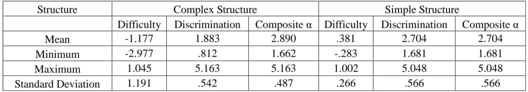
Page Table 1. Test Quality Table……….…..37 Table 2. Experimental Conditions for Simulation Study ……….…..39 Table 3. Descriptive Statistics for the R-RUM ……...……….…...59 Table 4. Descriptive Statistics for the 2PL CMIRT Model .………...……….…...60 Table 5. Descriptive Statistics for Test Quality

Definition for High-quality Test When r=.2...……….…………...64 Table 6. Descriptive Statistics for Test Quality

Definition for High-quality Test When r=.5………..…..……...…..…..…64 Table 7. Descriptive Statistics for Test Quality

Definition for High-quality Test When r=.9………..………...65 Table 8. Descriptive Statistics for Test Quality

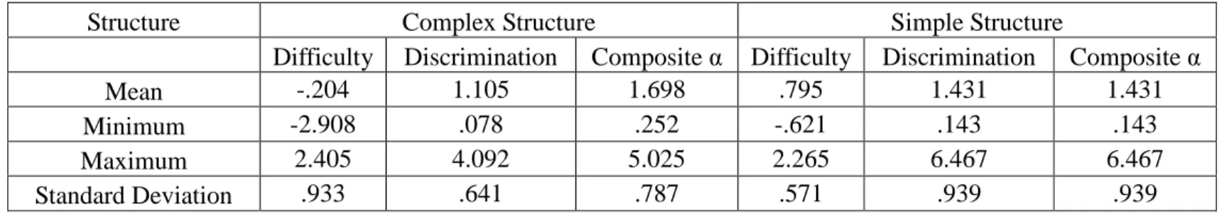
Definition for Medium-quality Test When r=.2 …...………....65 Table 9. Descriptive Statistics for Test Quality

Definition for Medium-quality Test When r=.5 ..…...….…..………....66 Table 10. Descriptive Statistics for Test Quality

Definition for Medium-quality Test When r=.9 ….….…….………….66 Table 11. Descriptive Statistics for Test Quality

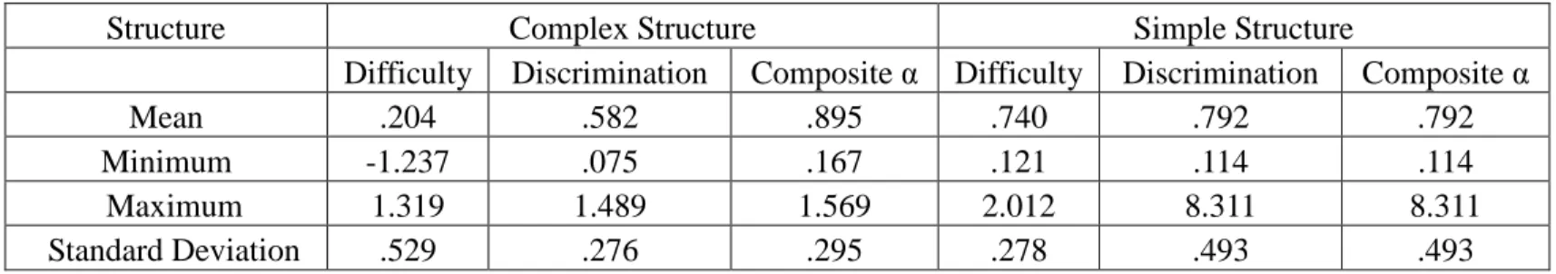
Definition for Low-quality Test When r=.2 …...………...…...67 Table 12. Descriptive Statistics for Test Quality

Definition for Low-quality Test When r=.5.….………..…...…67 Table 13. Descriptive Statistics for Test Quality

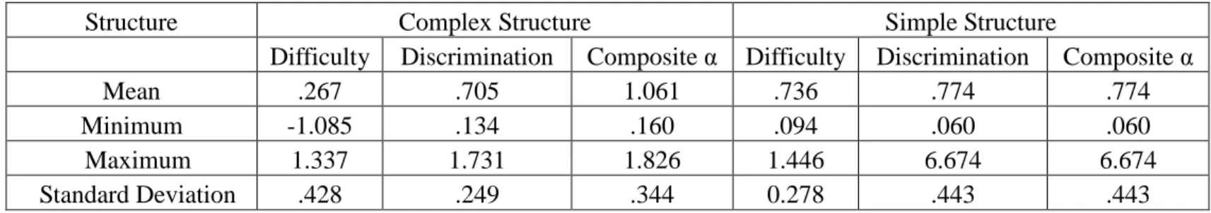
Definition for Low-quality Test When r=.9………..…...……..….68 Table 14. Descriptive Statistics for the Relation between Item Parameters of the Two Models in Case of High-quality Test, Complex Structure…...……..72 Table 15. Descriptive Statistics for the Relation between Item Parameters of the Two Models in Case of Medium-quality Test, Complex Structure………72

Table 16. Descriptive Statistics for the Relation between Item Parameters of the Two Models in Case of Low-quality Test, Complex Structure…..……...73 Table 17. Descriptive Statistics for the Relation between Item Parameters of the Two Models in Case of High-quality Test, Simple Structure………73 Table 18. Descriptive Statistics for the Relation between Item Parameters of the Two Models in Case of Medium-quality Test, Simple Structure…...….74 Table 19. Descriptive Statistics for the Relation between Item Parameters of the Two Models in Case of Low-quality Test, Simple Structure……….…...74 Table 20. Descriptive Statistics for Recoverability of Item Parameters of the Two Models in Case of High-quality Test, Complex Structure…...….….…...77 Table 21. Descriptive Statistics for Recoverability of Item Parameters of the Two

Models in Case of Medium-quality Test, Complex Structure .…...…...77 Table 22. Descriptive Statistics for Recoverability of Item Parameters of the Two

Models in Case of Low-quality Test, Complex Structure….…………...78 Table 23. Descriptive Statistics for Recoverability of Item Parameters of the Two

Models in Case of High-quality Test, Simple Structure.…...………...78 Table 24. Descriptive Statistics for Recoverability of Item Parameters of the Two

Models in Case of Medium-quality Test, Simple Structure ...….….79 Table 25. Descriptive Statistics for Recoverability of Item Parameters of the Two

Models in Case of Low-quality Test, Simple Structure ..…..…..……79 Table 26. Percentage of Raw Agreement between the Two Models…….…..…….…82 Table 27. Kappa between the Two Models .……...……….…...83 Table 28. Percentage of Agreement with the True Attribute Patterns ...…………...85 Table 29. Kappa-based Agreement with the True Attribute Patterns ...………...…86

LIST OF FIGURES

Page

Figure 1. Simple Structure .………20

Figure 2. Factorially Complex Structure…....………..21

Figure 3. Flow Chart for Simulation Study 1…....………...………46

CHAPTER I INTRODUCTION

Traditionally, testing industries have focused on constructing measures to assess a single dimension. The test is assumed to measure only one latent or unobserved ability or skill via the measured variables or items. Each examinee is rank ordered based on the total item scores or a single continuous latent ability and therefore only a single score is reported. Such reports have been widely used for high-stake decisions such as college admissions, scholarship awards and even graduation. As a result, researchers and practitioners have applied various statistical tools to verify that only one latent ability is present in the data structure.

Despite its parsimonious nature, traditional scaling of examinees has some limitations. Most psychological and educational tests measure multiple skills and the unidimensionality assumption cannot be met under these circumstances (Hambleton & Swaminathan, 1985). In addition, it falls short of cognitive psychology in the twentieth century. Cognitive psychometrics involves measurement models assessing high-order thinking, which is related to a set of skills. It is commonly agreed that research in high-order thinking is fundamental to the testing industry, as many tests are based on cognitive problem-solving skills (Gierl, Leighton, & Hunka, 2000). As a summative assessment model, traditional modeling, such as unidimensional item response theory (IRT) models, might be appropriate. However, traditional assessment is limited in its ability to provide any formative feedback for improving instruction,

learning and curriculum development. Principals, teachers and educators need more informative reports for classroom instructions and intervention programs. This urgent public demand is culminated in the No Child Left Behind Act (2001), which explicitly calls for ‘interpretive, descriptive and diagnostic reports’ and the use of assessment results for improving students’ academic achievements. Whereas both forms of assessment are necessary, one during the learning and teaching process and the other at the end of the instruction, formative assessments are more useful diagnostically at the classroom level throughout the course of instruction. In the simplest case,

formative assessments should determine mastery or non-mastery for a set of K skills. Recently, a variety of probabilistic latent class models have been developed for cognitive diagnostic purposes. These models assume that classes are defined by a set of discrete latent abilities, either binary or multicategorical. Each of these IRT-based cognitive diagnostic models (ICDMs) has an item response function (IRF) that

predicts the probability of the correct response for each item, given the attribute status of each examinee on each skill. As in IRT, the use of an IRF enables researchers to evaluate the quality of test items through the evaluation of the item parameters. Once an appropriate model is selected, each examinee’s profile is produced.

As an alternative for cognitive diagnosis, some researchers have pointed out that other IRT-based continuous latent models parallel the above discrete ICDMs. Contrary to the discrete ICDMs, these models place each of the underlying ability distributions on a continuum. DiBello, Roussos and Stout (2007) and Stout (2007) discussed these continuous models as possible psychometric models for cognitive diagnosis. Among these models, the application of multidimensional item response

theory (MIRT) models is common in research. For instance, Applied Psychological

Measurement devoted the winter issue of 1996 to research in MIRT models. Instead

of providing an estimate of a profile defining which attributes (or skills) have been mastered (i.e., a mastery profile), MIRT models produce factor scores. Therefore, if one were interested in determining which skills should be improved, further research must be performed to choose some factor score for each skill, at and above which the examinees are classified as masters and below which the examinees are classified as nonmasters. Consequently, if research or assessment is based on the factor scores from MIRT models, it is important to research how these conclusions about cognitive status of examinees compare to those from the ICDMs.

Both types of models, MIRT models or ICDMS, can be classified according to skill interactions into compensatory models and noncompensatory or conjunctive models. Compensation means that higher values on one skill can offset the lower values on other skills when calculating the probability of the correct response to an item. The extreme case of a compensatory model is the disjunctive model, which means a certain minimum on ONLY one of the relevant attributes is necessary to compensate for the lack of ability on all other skills for the correct response of the item. Noncompensation or conjunction means certain minimums on all skills are necessary for a high chance of a correct answer of the item. Anyone not having a minimum ability for at least one attribute will lack the ability to answer the item correctly. Having a higher ability in one attribute is NOT sufficient to compensate for the lower ability in other attribute(s) and to answer the item correctly (see Chapter II for more details).

The vast arrays of the psychometric models for cognitive diagnosis and their different ways to express cognitive complexity (e.g, underlying latent distributions, skills interaction, etc) make model selection difficult for accurate formative

assessments. If the selection is to be made among models differing only in scale assumptions, this might only pose the challenge of selecting some set of some factor scores from MIRT models to evaluate the examinees cognitively. If the selection is made among models differing only in skill interactions, this might only pose the challenge of determining the type of skill interactions to provide cognitive feedback. If the selection is to be made among models differing in both scale assumptions and skill interaction (compensatory or noncompensatory), this would pose the challenge of determining the type of skill interactions for cognitive evaluation of examinees in addition to the challenge of determining a reasonable set of cut points. In the latter case, it is expected that the cognitive evaluation of examinees will be different with a noncompensatory ICDM versus a compensatory MIRT or a compensatory ICDM versus a noncompensatory MIRT.

It is always difficult to select a reasonable psychometric model because of the challenge of identifying how the skills interact with each other—across items, individuals, groups and forms. In addition, it is not always clear whether the true underlying distributions of abilities are discrete or continuous. However, if in

application, final decisions based on cognitive feedback are similar even when using different models, then model selection may be based on an underlying theory without a focus on how these decisions will impact ultimate decisions for examinees. Due to the recency of the cognitive diagnosis, there has been limited research concerning the

comparison of the ICDMs and MIRT models for cognitive diagnostic purpose.

Therefore, it is the research goal of this study to compare the two types of models and investigate if model selection can influence final decisions that may be made for an examinee.

For the purpose of the current study, two models with different scale

assumptions and different skill interactions—one compensatory MIRT model and one noncompensatory ICDM model—were chosen (see Chapter II). The purpose of the current study is to determine how comparable the two models are with respect to the cognitive evaluation of the examinees. The two models have different assumptions about attribute scale and skill interactions. Therefore, it is necessary to identify what technique is most appropriate to compare the two different models. In chapter III, a technique is described such that the two models yield the most consistent evaluation of the examinees. Next, based on this technique, the models are compared with respect to how much the two models agree for cognitive diagnostic purposes. To address these goals, a simulation study was performed. Three factors—test quality, the Q-matrix (Tatsuoka, 1983) structure and the correlation between the attributes—were chosen in the simulation study. However, as the ICDMs are recently developed, its relationship with MIRT models is still unclear. Therefore, a preliminary simulation study must be performed to investigate the relationship between the two models. The relationship between the two models means (1) if they define test quality in the same way and (2) what the relationship between the item parameters of the two models is. It is possible that the two models differ in their definitions of test quality, but the item parameters of the two models might be associated with each other.

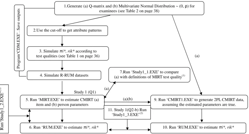
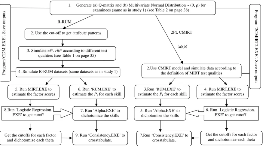
Chapter III describes in detail the questions and methodologies about the initial simulation study used to establish a definition of test quality of the ICDMs and MIRT models so that these two methodologies can be fairly compared on the final research goals. Two flowcharts (Figure 3 and Figure 4) are provided to illustrate the simulation procedures. Chapter IV discusses the initial study and chapter V addresses the final research goals.

The answers to the initial study will facilitate the understanding of the relationship between the ICDMs and MIRT models, which will be used to ensure a fair comparison between the models based on test quality. The answers to the final research goal will provide information about the importance of model selection for cognitive feedback. As the demand and the need for cognitive assessment are

increasing rapidly, model selection is becoming more and more crucial for formative assessment to be popular (DiBello & Stout, 2007; Bolt, 2007). If model selection does not impact the outcome related to examinees’ cognitive status, it is possible for

popular models to be used without affecting the results. If model selection does impact the outcome, the study is helpful to identify situations where the two models agree or disagree consistently. The results from the final research goal will also provide insight into the feasibility of using MIRT models for cognitive classification of examinees.

Chapter II provides a discussion of the ICDMs and traditional analytic models including the MIRT models. The review on different skill interaction is discussed and the comparison of the two selected models is provided. Chapter III discusses the questions, methodologies and statistics of each simulation study. Chapter IV deals

with the preliminary study and the final research goal of the study. Chapter V ends the study with conclusions and future directions.

CHAPTER II LITERATURE REVIEW

Cognitive diagnosis, skill assessment or skill profiling refers to the partitioning the latent multidimensionality into discrete latent attributes and evaluating the examinees with respect to their status of mastery of each attribute (Hartz, Roussos & Stout, 2002). In the literature on cognition, ‘attribute’ is used interchangeably with ‘dimension’, ‘factor’, ‘skill’, ‘subskill’ and ‘latent ability’. In this study, the ICDMs refer only to the stochastic models recently developed. All of these models assume that attributes are discrete and are discussed in detail in Section 2.1. The traditional continuous latent variable models, referred as traditional factor analytic models, are presented in Section 2.2. In both sections, conjunctive models and compensatory models are discussed. Section 2.3 includes the definitions and literature review of compensation and noncompensation. The last section presents the comparison of the selected models.

2.1 IRT-based Cognitive Diagnostic Models

IRT-based cognitive diagnostic models (ICDMs) recently developed all define the probability of correctly answering an item as a function of a set of discrete attributes measured by the item. In addition, the models require that a Q-matrix has been defined with elements qik, where 1 indicates that the kth attribute is required by the ith item and 0 otherwise. In most cases, the Q-matrix is assumed as fixed and is determined by content experts. In addition, most ICDMs assume that only mastery of

those attributes specified by the Q-matrix is necessary for the correct responses. These ICDMs can be classified according to skill interaction into noncompensatory or conjunctive and compensatory models. The conjunctive models are presented first and the compensatory models are presented next.

Conjunctive Models

Reparameterized Unified Model (RUM, Hartz et al, 2002, also referred to as the

Fusion model) was defined based on the Unified Model (DiBello, Stout & Roussos, 1995). The Unified Model is among the first cognitive models to acknowledge that the Q-matrix is an incomplete representation of all the cognitive requirements for the test, thus differentiating the Unified Model from most early cognitive diagnosis models. Specifically, the Unified model includesPC_l(θj), where θj is a single

continuous ability parameter as a unidimensional projection of examinee j’s relevant attributes outside those defined in the Q matrix (using a Rasch model with different parameters—c ). The problem with the Unified Model is that it is not estimable _i

because there are 2ki+3 parameters (k = the number of attributes required by the item) for each item i and thus, the parameters are not identifiable.

Hartz (2002) developed the RUM (Fusion Model) out of the Unified Model. She reparameterized the Unified model so that it was estimable and she retained the interpretability of the parameters. The reparameterized model has 2+Ki parameters per item, where Ki represents the total number of required attributes for an item. The R-RUM defines the probability of a correct response P(Xij =1/αj,θj)as:

( 1/ , ) [ (1 ) ] ( ) 1 * * j c q ik K k i j j ij i ik jk P r X P

α

θ

π

θ

π

π

∏

=

=P(correctly applying all item i required attributes given q_ik=1 for all item required attributes), which is the probability of giving a correct answer to all the attributes given that an examinee j is a master of all the traits (k=1,…K) related to item i. ) 1 / 1 ( ) 0 / 1 ( * = = = = = jk ijk jk ijk ik Y P Y P r α α

which is interpretable as item i discrimination parameter for attribute k or the penalty for not mastering attribute k

ci = the amount that correct item performance requires θj, in addition to the required Q attributes; referred to as the completeness index for item i. The ranges of the parameters are 0 ≤ *

i

π ≤ 1, 0 ≤ * ik

r ≤ 1, 0< ci <3. For the

discrimination parameter, rik* is 1 when the item does not require the k

th

attribute and 0 when the discrimination is maximum. The additional ability,θj, is assumed to be

continuous, ranging from -∞ to +∞ . As the value of θj approaches infinity,

) ( _j

Cl

P θ approaches to 1 for all values of c . When the value of c_i i is approximately 0, the different values of _C ( _j)

l

P θ will influence the item response function. The estimation of the RUM was solved using a Markov Chain Monte Carlo (MCMC) algorithm and a stepwise parameter selection procedure.

The RUM is among the most common ICDMs studied (e.g, Jang, 2005). Hartz (2002) applied the model to PSAT/NMQT for the purpose of improving students’ performance on SAT. Jang (2005) also applied the RUM comprehensively to ETS-TOEFL standardized testing. Jang constructed the Q-matrix by combining the characteristics of the items with the results from DIMTEST and DETECT. The insignificant item parameters were eliminated and the program for the RUM was rerun on the data, using the modified Q-matrix. The follow-up study, surveys and interviews, was conducted on a sample of 28 students and two teachers, to

cross-validate the diagnostic reports. Roussos, Hartz and Stout (2003) applied the RUM to the math section of American College Testing’s assessment.

The Reduced RUM (R-RUM, Hartz et al, 2002, Henson & Douglas, 2005; Fu,

2005) The R-RUM is a simplified version of the RUM with the additional ability,

j

θ , removed. With the non-Q attributes (PC_l(θj)) removed, it is implicitly

acknowledged that the Q-matrix is a complete representation of the skills required for the test or the non-Q attributes are insignificant. The interpretations of the remaining parameters are the same as in the RUM and thus the probability of a correct response is defined as: ik jk qik K k i j ij

r

X

P

)

/

1

(

α

π

∏

=

=

Henson & Douglas (2005) applied this model in the study on the ICDM test discrimination indices.

The NIDA Model (noisy inputs, deterministic “and” gate, Junker and Sijstma, 2001; Maris, 1999) In the NIDA model, the probability of a correct response is:

P(X_ij =1/α_j,s, g) = jk k jk qik K k k

g

s

)

]

1

[(

∏

−

Where s_k = P(η_ijk =0/α_jk =1,q_ik =1), a slipping parameter gk = P(

η

α

η_ijk, a latent variable defined at attribute level, with 1 indicating the examinee

j has correctly applied attribute k on item i and 0 otherwise.

The NIDA model predicts the probability of giving a correct response as the product of slipping and guessing parameters. In the model, s_k is an error probability that an examinee incorrectly applies attribute k when in fact, he or she is a master of that attribute and g is the probability that an examinee correctly applies attribute k _k

when he or she is a non-master of that attribute. Because the slipping and guessing parameters are defined at the attribute level, only the Q-matrix distinguishes difference among items and no item specific parameters are defined. Maris (1999) gives another version of the NIDA model with the parameters estimated for each item and so the probability of a correct response is defined as:

P(X_ij =1/α_j,s, g) = jk ik jk qik K k ik

g

s

)

]

1

[(

∏

−

de la Torre and Douglas (2004) applied the NIDA model for assessing the skills used in mixed number subtraction. Based on the content and the problem-solving characteristics of the 20-item test, they identified an eight-skill Q matrix for fraction subtraction.

The DINA Model (deterministic inputs, noisy “and” gate, Junker & Sijstma,

2001; Macready & Dayton, 1977; Haertel, 1989). The DINA model defines the probability of a correct response as a function of two probabilities based on whether the examinee has mastered the required attributes for the ith item. Specifically,

( 1/ , , ) (1 ) ij (1 ij) i i j j ij ij s g s g X P = ξ = − ξ −ξ (2.5) Where qik jk K ki ij

α

ξ

= , which is an indicator of whether examinee j has mastered all the required attributes for item i, with 1 indicating the mastery of all of the item’s required attributes and 0 nonmastery of at least one attribute;

) 1 / 0 ( = = = _{ij ij} i P X

s ξ , a slipping parameter; defining the probability that the examinee j, a master of all traits, incorrectly responds to the item.

) 0 / 1 ( = = = _{ij ij} i P X

g ξ , a guessing parameter, meaning that a nonmaster of at least one attribute, ‘guesses’ and correctly responds to the item.

The DINA model constrains (1−s_i)to be greater thang . The model simplifies _i

examinees into two groups—masters and non-masters. In the non-master group, the examinees missing one attribute are equivalent to those missing all the attributes. Zhang (2006) applied the DINA model for differential item functioning (DIF) study. In the study, Zhang manipulated the item parameters for the different groups and completed a DIF analysis on simulated data and using real data. In addition to the NIDA model, de la Torre and Douglas (2004) also applied the DINA model for the cognitive diagnosis of the skills used in mixed number subtraction. Recently, based on

real data, de la Torre and Lee (2007) used the DINA model to explore the relationship between the ICDMs, classical testing theory and IRT indices.

Compensatory Models

In the following section, examples of compensatory models are introduced. They include the compensatory RUM (Hartz, 2002), NIDO (Templin, Henson, Douglas, 2006) and a disjunctive model—DINO model (Templin & Henson, 2006). As defined in the previous chapter, a disjunctive model is an extreme case of the compensatory model in the sense that the competency on ONLY one skill is enough for the correct answer of the item. Last are the LCDM (Henson, Templin, & Willse, 2008) and the GDM (von Davier, 2005), the two general versions of compensatory and noncompensatory model as was shown by Henson, Templin and Willse (2008) through their introduction of the log-linear cognitive diagnostic model (LCDM).

Compensatory RUM (Hartz, 2002). The compensatory RUM is a compensatory

version of the R-RUM, where the probability of a correct response is defined as:

∑

∑

whereβi= the intercept parameter interpreted as the baseline log-odds of getting the

item correct for examinees not mastering the skill.

γik=the increased log-odds of getting the item correct for each mastered

Q-matrix indicated skill

Therefore, for those who are nonmasters of all the Q-matrix specified attributes, the probability of the correct response is a function of the intercept parameter. This

model was later defined as a special case of the generalized diagnostic model (GDM, to be discussed, von Davier, 2005) and was applied to TOEFL test (von Davier, 2005).

The NIDO Model (noise input deterministic ‘or’ gate, Templin, Henson

&Douglas, 2006) Based on NIDA model, Templin, Henson and Douglas (2006) developed a compensatory model so that the probability of a correct response:

∑

∑

whereβk= the threshold of getting the skill correct for examinees not mastering the

skill;

γk= the skill level discrimination parameter

Notice that the NIDO model defines the probability of a correct response using only two parameters per skill. Like the NIDA model, this model does not have parameters at the item level and so the item parameters will have identical values within the same skill. As a result, the probability of getting the item correct will be identical for items with an identical Q-matrix entry.

The DINO Model (deterministic input noise ‘or’ gate, Templin & Henson, 2006)

Based on the DINA model, Templin and Henson (2006) developed a disjunctive model. Similar to the notation

ξ

∏

Incorporating this notation into the DINA model, the conjunctive model now becomes a disjunctive model, predicting the probability of a correct response as a function of the slip and guessing parameters:

( 1/ ) (1 ) ij (1 ij) i i ij ij s g X P =

ω

The Log-linear Cognitive Diagnostic Model (LCDM, Henson, Templin & Willse,

2008) The LCDM is a flexible log-linear model that can fit many of the

noncompensatory or compensatory models discussed above. First, give a general model when the number of attributes is 2 (K=2). The LCDM predicts the probability of correct response as:

) exp( 1 ) exp( ) / 1 ( 2 1 12 2 2 1 1 2 1 12 2 2 1 1 i i i i i i i i ij X P β α α γ α γ α γ β α α γ α γ α γ α − + + + − + + = = (2.10)

where γ_i12 represents skill interactions with a value greater than 0 indicating the noncompensation and 0 or less indicating compensation.

γ_ikis the discrimination parameter for each attribute related to item i.

β_i is the intercept parameter interpreted as the probability of a correct response for those who are nonmasters of the required skills.

Notice this is a model for dichotomous data. Using examples, Henson, Templin and Willse (2008) demonstrated how the LCDM could fit compensatory RUM, DINA,

DINO and reduced RUM. Perhaps more importantly, the LCDM provides a parameterization for assessing the differences between each model and thus can be used to identify a reduced model such as the models previously described. The authors also performed MCMC estimations on a real dataset. The results from the LCDM estimation indicated that some items were consistent with the DINA, one item was consistent with the DINO and some items were consistent with compensatory RUM.

The Generalized Diagnosis Model (GDM, von Davier, 2005) The GDM is a

general and flexible version of the ICDMs. The GDM can provide parameter estimates for multiple item types (dichotomous and ordered responses) with multiple latent ability types (either dichotomous or approximately continuous). With the GDM, the Q-matrix entries can be either dichotomous or polytomous skills. Within the class of the GDM, both compensatory and noncompensatory ICDMs may be specified (Henson et al, 2008). The GDM predicts the probability of correct responses by:

)] , ( exp[ 1 )] , ( exp[ ) , , , / ( 1 . . jk ik m y T yi yi jk ik T xi xi i i i a q h a q h q a x X P i

∑

where h(qi,a)=(h1(qi,a),...,hk(qi,a)) is a vector of functions )

,..., ( _{xi1 xiK}

xi γ γ

γ = , (2k-1) dimensional slope parameters to determine the contribution of each non-zero Q-matrix entry.

β_xi, the real-valued difficulty parameters

When h(q_i,a)=α_ik×q_jk, the compensatory RUM is a special case of the GDM. With the exception of the RUM, all the above ICDMs can be modeled with the GDM

(Henson et al, 2008). However, the GDM can approximate the RUM (Henson et al, 2008). Notice when k in equation 2.11 is 1 and α_j is defined as a continuous latent variable with normal distribution, the GDM is an expression for the two-parameter logistic IRT model.

The GDM was applied to both the simulated data and the real data (von Davier, 2005). For the simulated data, the classification accuracy across four skills using Cohen’s kappa was above .85 across five different replications. The application was done on TOEFL Internet-based testing pilot data with two forms (Form A and B) and two sections (Reading and Listening). The Q-matrices were supplied by the experts. Seven out of eight skills were strongly related to the overall ability obtained using the traditional 2PL IRT model. The skill profile indicated four highly correlated skill classifications for the Listening section and the three highly correlated skill classifications for the Reading section.

The popular ICDMs in the literature have been commonly conjunctive models, such as the RUM and DINA. These ICDMs are IRT-based in the sense that they share some similarities with the IRT models in their assumptions. The ICDMs assume local independence conditional on the latent ability (i.e.,αj). Specifically, they assume that

after conditioning on an examinee’s abilities, the responses of an examinee to different items will not influence each other and that examinees from the same group (i.e., the same αj) should have the same expected response pattern. In the ICDMs,

monotonicity means that the probability of correctly responding to an item is non-decreasing in each coordinate of the attributes with all other coordinates held

fixed (Junker & Sijtsma, 2001).

2.2 Traditional Factor Analytic Models Linear Factor Model

Factor analysis started with Charles Spearman (1904). He proposed the one-factor theory, which assumed the test measured one general factor in common, g, general intelligence. He suggested that all human intellectual activities have this general factor in common. In addition, the more two tests have in common with the general factor, the higher their correlation would be. He also proposed a second factor,

the specific factor. This factor was only specific to a single activity or variable and not

correlated with the general factor. Its presence could reduce the correlation between the tests. Therefore, within a test, it is the general factor, a factor universal to a person’s ability, that accounts for the correlation among the items.

Some researchers did not agree with the one-factor model. Thurstone (1938) is one of the famous proponents of the multiple factors. Analyzing the responses from 240 volunteer students on fifty-six tests, he identified nine independent factors. Later, Thurstone (1941) completed a second study and found the same factors present. It was Thurstone who put forward the concept of ‘simple structure’, a very important concept in factor analysis. Simple structure describes a test where each item loads on only one dimension. Graphically, simple structure can be represented as follows:

Figure 1. Simple Structure

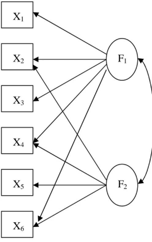
As opposed to simple structure, a test is factorially complex when a measured variable is related to more than one factor or an item is measured by more than one factor (refer to Figure 2).

X1 X2 X3 X4 X5 X6 F1 F2

Figure 2. Factorially Complex Structure

Generally, for each person, the factor model may be expressed:

x_i =µ_i +Λ_ikf_k +ε_i (2.12)

In this model, xi is a column vector of the measured variable i, or responses to items.

The constant µi represents the ith item’s difficulty. Λis a (i×k) matrix of factor loadings, representing the amount of information that each item contains about each factor k related to item i. Factor loading describes discriminating power of the item. For standardized data, factor loadings range from 0 to 1 with 1 indicating maximum discrimination and 0 indicating no relation with the factor. fk is a column vector of

latent variables and єi is a column vector of unique factors. When K>1, it is a multi-factor model. When K=1, Λ is a column vector and the equation (2.12) is the

X1 X2 X3 X4 X5 X6 F1 F2

expression for classical testing theory (CTT) (f corresponds to T, unobservable true score in CTT).

Item Response Theory Models

In the above linear factor models (equation 2.12), the observed variable is predicted based on a linear combination of a set of latent variables. However, equation 2.12 is not appropriate for dichotomous item responses. When equation 2.12 is a one-factor model, the model has the following limitations. First, the assumption of linearity between the item and the latent factor cannot be met (McDonald, 1999). It is possible that equation (2.12) yields a probability less than 0 if the factor score is too small, and a probability greater than one if the factor score is large enough. Second, it assumes that error and factor are independent of each other and that the error variance is constant across all values of factors. When K in equation 2.12 is greater than 1, the linear factor model is a multiple-factor model. When applying the linear multiple-factor model to educational measurement, the same limitations associated with the linear one-factor model still exist except that each factor has its constant error variance across the values of the latent ability.

In educational measurement, one method to overcome these limitations is by using a nonlinear transformation such as is commonly used the popular IRT models. IRT models have some favorable features—such as the invariance of both item parameter estimates and ability estimates and the ability to predict the probability of the correct response for an examinee to an item given the item parameter(s). In addition, the standard error of measurement, that is the inverse of square root of information, varies across ability. The relationship between the probability of a correct

response and the latent ability is monotonic, that is, as ability increases, the probability of the correct response increases. In IRT models, the common models are either logistic models or the normal orgive models (Lord, 1952) and they differ approximately by a constant, but the logistic IRT models are more popular due to their simplicity in computation. IRT models can be classified into three-parameter (3PL) model (Birnbaum, 1968), two-parameter (2PL) model (Birnbaum, 1968) and one-parameter (1PL) model (Rasch, 1961). Because the focus of the current study is about cognitive diagnosis, only the multidimensional item response theory (MIRT) models are discussed.

Multi-dimensional IRT models The multidimensional IRT (MIRT) models

predict the probability of the correct response for an item as a function of a set of item parameters as well as a vector of the given ability levels. In MIRT, there are two classes of popular models—the compensatory MIRT models (CMIRT, Reckase & McKinley, 1991) and the noncompensatory MIRT models (NCMIRT, Sympson, 1978).

Noncompensatory Multidimensional IRT (NCMIRT) Model (Sympson, 1978)

Each dimension in the NCMIRT has its own difficulty parameter (dik) and its own

discrimination parameter,a , for the k_ik th trait related to item i . Higher values of the difficulty parameters indicate more difficult items and lower values indicate easy items. The multiplicative nature of the noncompensatory models prohibits an examinee from compensating for a low ability on one dimension by having a high ability on another or the other dimension(s). The most complex model of this family of NCMIRT is the 3PL NCMIRT, where the probability of a correct response is:

) ( ) ( 1₁ ) 1 ( ) , , / 1 ( ik jk ik ik jk ik d a d a K k i i ik ik j ij e e c c d a x P ₋ − = + ∏ − + = Θ = _θ θ (2.13) The 2PL NCMIRT model is a simpler version of this 3PL model with c i

constrained to zero for i=1,…,I. The 1PL NCMIRT model is the simplest version of equation (2.13) with the discrimination parameters constrained to unity and guessing fixed at zero.

Compensatory Multidimensional IRT (CMIRT) Model (Reckase & McKinley,

1991). Unlike the noncompensatory model, the CMIRT model has a vector of discrimination parameters, one difficulty parameter and one guessing parameter per item. The negative values of the difficulty parameter (d ) indicate the more difficult i

items while the positive values suggest the easier items. Regardless of the number of dimensions, there is only one item difficulty parameter and one item guessing parameter. The 3PL CMIRT model, as is indicated, includes the discrimination

parameter a for each skill k related to item i, a guessing parameter (ci), and a difficulty parameter (d ) for all dimensions. Specifically, the 3PL multidimensional logistic _i

model is: i d jk K k ik a i jk K k ik e e c c d a x P d a i i i ik j ij ₊ = ∑ = + − + = Θ = + ∑ θ θ 1 1 1 ) 1 ( ) , , / 1 ( (2.14)

The discrimination parameters in (2.14) are constrained to be positive and the length of the item vector is equal to the amount of multidimensional discrimination (Ackerman, 1994; Reckase & McKinley, 1991). Due to the additive nature of the elements in the exponent, the examinees having a low ability on one dimension can

benefit from having a high ability on another or other dimension(s).

As to the 2PL CMIRT (Reckase, 1985), the guessing parameter is set to zero. Thus the model becomes:

i d jk K k ik a i jk K k ik e e x P d a j ij + = ∑ = + = Θ = + ∑ θ θ 1 1 1 ) / 1 ( (2.15)

Note that this is equivalent to the nonlinear factor analysis with a logit link as previously described (Christoffersson, 1975; McDonald, 1967).

With the 1PL or the Rasch CMIRT model, the guessing parameters are set to zero and the discrimination parameters are constrained to unity.

These two types of the models can be rewritten as a generalized multidimensional item response theory (GMIRT) model (Ackerman & Bolt, 1995):

] [ ] 1 [ ) , , , / ( 1 1 1 ijk ijk K k ijk K k f K k f f ik ik j ij e e e b a x P ∑ = ∑ ∑ ∑ + + = Θ = = µ µ (2.16)

where fijk=aik(θjk −dik). In equation (2.16), u is a weight with 0 representing

fully compensatory model and 1 fully noncompensatory model, but any value between 0 and 1 indicates the varying degree of compensation required by the

attributes. This model may be viewed as a general expression of the MIRT models and the unidimensional IRT models. In addition, a guessing parameter could be included to define a three-parameter model.

In educational measurement, the nonlinear factor model and the MIRT models, are more popular. The 1996 winter issue of Applied Psychological Measurement was

devoted to research of MIRT models. As shown in the next section, a large amount of research has been completed using MIRT models in educational measurement. As members of the IRT family, the relationship between MIRT models and the linear factor analysis has been established (Christoffersson, 1975). Due to its popularity, there may be some circumstances where the MIRT model would be selected to provide diagnostic information as to the ICDMs. Therefore, it is the goal of the current study to compare these two types of models to investigate how consistent the two models are with respect to cognitive diagnostic and to identify the situations where they are comparable.

2.3 Literature on Compensation and Noncompensation

The concepts of compensation and the noncompensation or conjunction was first introduced by Coombs (1964), Coombs and Kao (1955) and Johnson (1935). Under conjunctive model, the joint abilities of all attributes are necessary for answering the item correctly. Anyone lacking the ability in one attribute will lack sufficient knowledge to answer the item correctly and so will most likely miss the item. That is, having a higher ability on one attribute is NOT sufficient for

compensating for the lower ability in other attribute(s) and answering the item correctly.

In contrast, compensatory models allow for a higher ability on one attribute to compensate for the lower ability on other attribute(s), thus increasing the probability of getting the item correct. Popular compensatory models include the linear factor models and some MIRT models with additive properties. Unlike equation 2.13, which is multiplicative across dimensions, equation 2.14 to equation 2.15 are additive across

the dimensions. Although additive models in the literature assume a compensatory relationship between the latent abilities and the response holds, other models, such as a disjunctive model, can also be considered compensatory. Disjunctive model require that a minimum competency on ONLY one attribute is enough for the correct answer. Apart from disjunctive model, disjunctive processing may also be represented by the negative interaction term (Henson, Templin, & Willse, 2008).

The compensatory and noncompensatory models are different from each other in the nature of cognition. The implied cognitive assumption of compensation is that the complete mastery of the Q-matrix skills is not necessary for the correct answer of the item. Instead, an ability at or above a minimum level on any of the relevant skills plays a dominant role in answering the item correctly (in the disjunctive case, it is enough to have a minimum on one skill for the correct response of the item). The cognitive assumption of noncompensation is that all the skills relevant to the item are necessary for the correct response of the item. Empirical evidence supports both types of models.

Some research found compensation outperformed noncompensation while other research found compensation and noncompensation were comparable or

noncompensation was superior. For example, Simpson (2005) used the GMIRT model to investigate the relationship between noncompensatory processing and the task of matrix completion. She found u , an indicator of the degree of compensation, in the

GMIRT model,was greater than 0, supporting the compensatory processing in the cognitive solution of matrix completion. Mislevy et al. (2002) found that compared with the conjunctive model, the compensatory model produced relatively high

reduction in posterior variance, indicating the compensatory model is a better fit. Comparing the compensatory model with the noncompensatory model, Van Leeuwe & Roskam (1991) found that a compensatory MIRT model provided better fit to LSAT data than a noncompensatory MIRT model.

Hambleton and Slater (1997) compared a compensatory policy with a policy combining compensatory and conjunctive components with respect to standard setting. Their results demonstrated that the compensatory policy increased the levels of

decision consistency and the levels of decision accuracy whereas the policy combining both compensatory and conjunctive components lowered the levels of decision consistency and the levels of decision accuracy. Under the policy with the conjunctive components, the candidates failed at a very high rate. Consistent with Hambleton and Slater’s results, Haladyna and Hess (1999) found compensatory strategies outperformed conjunctive strategies decisively in terms of reliability and rater consistency. Richter and Späth (2006), in their study of decision-making, found that people integrated information with other types of task-relevant knowledge in judgment and decision making, which was an indication of compensatory

decision-making.

On the other hand, some research does find both models are comparable or support the noncompensatory model. Way, Ansley and Forsyth (1988) simulated data using both compensatory and noncompensatory models. Their independent variable was the correlation between the dimensions and the dependent variable was the ability estimates. Their results showed that the observed score distributions for each model were comparable and the θ estimates were most highly related to the average of the

two θ parameters. In a study of the success of the graduate students (Nelson, Nelson & Malone, 2000), both the compensatory term and the conjunctive term were found to be significant predictors. Investigating geometric analogy solution as a function of systematic variations in information structure of the item, Mulholland, Pellgegrino and Glaser (1980) found that the best-fitting function was a nonadditive model (a conjunctive model) instead of a simple additive model (a compensatory model). In the study of teacher licensure, Mehrens and Phillips (1989) found that the conjunctive model was more appropriate when the purpose was to set a cut-off value for the minimal competence instead of predicting the degree of success. To study Korean high school students’ decision-making process, Hong & Chang (2004) conducted their study using ‘think-aloud’, tape-recording and observations and concluded that

students preferred the non-compensatory rules instead of the compensatory rules which allowed the trade-off among alternative strategies.

With the complexity of cognition, it is impossible for one model to be the best for all scenarios. Apart from cognition, many factors might influence which type of skill interaction might occur. These factors include assessment purposes, content areas, test designs, attribute structures, or different target populations. Skill interactions might vary across items, skills, test structures, individuals, groups and populations. It is quite possible that some data might be a mixture of compensation and conjunction. 2.4 Comparison of the R-RUM and the 2PL CMIRT

A common saying may depict the dilemma of psychometricians very precisely: “A person with one watch knows what time it is; a person with two watches is never quite sure.” The challenge becomes greater when there are many models available.

That is, models will have to be selected based on a compromise of model fit, the purpose of the models and some additional factors such as the assessment purpose and the way of reporting the cognitive status. However, when the measurement from two different models yields a similar interpretation, then one can make a selection based on personal preference, software availability or/and the assessment purposes. Thus, the goal of the current study is to investigate the effect of two different models on the final cognitive diagnosis of the examinees.

To make such a comparison, two models were selected—R-RUM and 2PL CMIRT model. When choosing the models, four factors were taken into consideration—model popularity, the substantive item parameter interpretations, skill interactions and attribute scales. Among the ICDMs, the conjunctive models are more commonly used such as the RUM, the R-RUM and the DINA (e.g. Hartz et al, 2002; Jang, 2005; Henson and Douglas, 2005). Among the traditional MIRT models, the CMIRT models are more often found to outperform the NCMIRT models (e.g., Bolt &.Lall, 2003; Mislevy et al, 2002). The R-RUM shares similar item parameter interpretations as the 2PL MIRT model. π_i* in the R-RUM, ranging from 0 to 1, can be interpreted as the conditional item difficulty parameter based on Q-matrix. It is closer tod , item difficulty parameter in the 2PL MIRT models. In the R-RUM, i

* ik

r is interpretable as item i discrimination parameter for attribute k, with 0 indicating the

maximum discrimination and 1 indicating no discrimination. This is somewhat similar

to a , discrimination parameter in the 2PL MIRT models. The rest of the ICDMs do _ik

When selecting models for comparison, all underlying assumptions were also considered. The R-RUM is a conjunctive model and the 2PL CMIRT is a compensatory model. The R-RUM assumes the underlying distributions are discrete while the 2PL CMIRT assumes each of the distributions is on a continuum. The 2PL CMIRT and the R-RUM aggregate all different assumptions and are, therefore, chosen for the research goal. If these two models can yield a similar interpretation about the cognitive status of the examinees, then the challenge of selecting a cognitive diagnostic model can be based on whichever model the psychometricians prefer (maybe, the customers prefer), what software is available, or/and whichever model fit the assessment purposes.

However, an initial challenge must be overcome before directly comparing the R-RUM with the 2PL CMIRT model with cognitive feedback. The R-RUM is newly developed and its relationship with the traditional MIRT models is unknown. A preliminary study is necessary to address the relationship between the two models. Two questions are related to the relationship between the two models: (1) how do the two models define test quality? (2) What is the relationship between the item parameters of the two models?

In Chapter III, Figure 3 is the flowchart to address the initial challenge

regarding the relationship of the two models with two specific questions. Notice that the results from the test quality of the two models will influence the comparability of these two models. Figure 4 provides the detailed simulation procedures to investigate if the two models can produce a similar interpretation of the cognitive status of the examinees. Included are also the research questions, the methods and the statistics

CHAPTER III METHODOLOGY

The purpose of the current study is to find out how comparable the ICDMs and the traditional MIRT models are with respect to cognitive feedback of examinees. For this purpose, the R-RUM and the 2PL CMIRT model are selected. The R-RUM is a noncompensatory model with discrete attributes and the 2PL CMIRT model is a compensatory model with continuous attributes. If these two models yield the similar results about the cognitive status of the examinees consistently across experimental conditions, then model selection can be based on the preference of the researchers or/and the clients in addition to software availability. However, unlike the R-RUM, which yields the probability of mastering each skill, the MIRT model produces continuous factor scores, and thus classification of examinees into masters and non-masters does not exist for the MIRT model. Therefore, first, a methodology is defined to identify a point, or a cut-off, for the factor scores so that examinees at or above this point are masters and examinees below this point are nonmasters. Specifically, assume that a common dataset is collected and fit by both the R-RUM and the 2PL CMIRT model. The R-RUM analysis of this data will result in estimates that can be directly used to classify examinees as a master of each attribute whereas the results from the 2PL CMIRT model for each attribute will be continuous scores for each examinee, with no direct way of determining how to transform the continuous

scores of the MIRT into dichotomous estimates of mastery/nonmastery. Therefore a method is described to determine a cutoff on the scale of the MIRT continuous abilities such that the agreement of mastery/nonmastery of the two models, when using the same dataset, is maximized.

Among the statistical tools, binomial logistic regression (thence referred as logistic regression) is used to convert the continuous values of the MIRT model to dichotomous outcomes. In logistic regression, independent variables can be interval, nominal or categorical, or a combination of all these and the dependent variable is dichotomous. Logistic regression can be used to predict the likelihood of having or not having the expected outcome given the independent variable(s). The property of logistic regression is that it is either monotonic increasing or monotonic decreasing. In the current study, the independent variable is the estimated continuous factor scores from the MIRT model and the dependent variable is the estimated mastery status (either master or nonmaster) when the R-RUM has been estimated using the same dataset. Thus, an examinee will be classified as a master on one θ when the predicted probability of the logistic regression is equal to or greater than .50. As the estimated continuous factor scores increase, the expected likelihood of being a master (i.e., the predicted probability of the dependent variable equaling 1 in the logistic regression) increases monotonically. Using logistic regression, the predicted

probability for the mastery status of each skill will be obtained given each continuous factor score. Those having a predicted probability at or above .50 are classified as masters and those below .50 are classified as nonmasters. Because the cut-off values

(i.e. .50) from logistic regression yield the most consistent cognitive evaluations of examinees between the two models, they are referred as ‘optimal’.

Provided that the previously described method will be used to compare the two models, the following paragraphs provide an explanation of the conditions selected to compare them in a simulation study. Because this is a simulation-based study about how comparable the two models are with respect to cognitive feedback given to examinees, factors in this study are considered if they are expected to affect the estimation of the examinees’ profiles (either continuous or dichotomous) either directly or indirectly. Section 3.1 discusses these conditions in detail.

3.1 Experimental Conditions

As was discussed, factors of the simulation studies are selected that are expected to affect the cognitive feedback of examinees. One important factor affecting the estimation of examinees’ cognitive status is test quality. Test quality directly influences the ability of a test to accurately estimate examinees’ profile, either continuous or dichotomous. Henson and Douglas (2005) redefined the test reliability or the test quality in cognitive diagnosis to be the accuracy of classification of examinees. Item discrimination, in the cognitive diagnostic models, measures the extent that an item provides information about the classification of each attribute. Items with high discrimination are more reliable at classifying examinees as masters or nonmasters. Simulation studies (Hartz et al, 2002; Henson & Douglas, 2005)

showed that test quality directly affects the correct classification rate of the examinees. A high-quality test has a higher correct classification rate. In contrast, a low-quality test has a higher misclassification rate. When test quality is low, two parallel tests will

not agree even if the true model is applied and so the agreement rate in this case must be low if two different models are compared when calibrated using the same dataset. If and only if the two models define test quality in the same way, the estimated factor scores of a master will be consistently higher than those of a nonmaster. On the contrary, if the two models define test quality differently, the implication is that one model is more reliable at classifying examinees. Therefore, comparisons cannot be made across the datasets simulated using the two different models. Comparisons can only be made on the datasets simulated using each model after running the estimation programs of the two models on the common datasets.

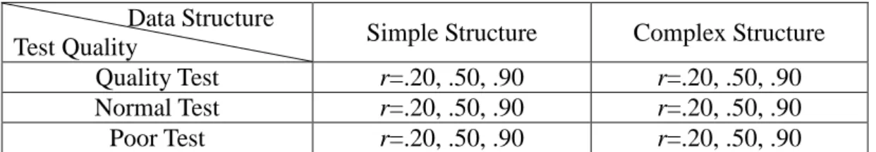
In this study, different test qualities—high, medium and low—are replicated. In the R-RUM, the items with high π_i* and low r_ik* are more informative about the attributes (Hartz et al, 2002; Henson, Douglas, 2005; Templin, Henson & Templin, 2008). To be more specific, Henson and Douglas (2005) defined high, medium and low quality tests in the R-RUM as follows:

1. High quality test: * i

π ~ ( .85, .95) and * ik

r ~ ( .10, .30) 2. Medium quality test: πi*~ ( .75, .95) and

* ik

r ~ ( .10, .90) 3. Low quality test: π_i*~ ( .75, .85) and r_ik*~ ( .40, .90)

In MIRT models, the test quality is related to the composite discrimination index, which is _ik2 K k c a a = ∑

= , where a_ik are from equation 2.13 to equation 2.16 (Ackerman, 1994). Higher values of a indicate the item is good at differentiating _c