Visualization and Analysis Techniques for Urban Microclimate Data Sets

for Urban Microclimate Data Sets

Vom Fachbereich Informatik der

Technischen Universität Kaiserslautern

zur Verleihung eines akademischen Grades

Doktor der Ingenieurswissenschaften (Dr.-Ing.)

genehmigte Dissertation

von

Kathrin Häb

Datum der wissenschaftlichen Aussprache:

17. Juli 2015

Prüfungskommission/Berichterstatter:

Prof. Dr. Jens Schmitt, TU Kaiserslautern (Vorsitz) Prof. Dr. Hans Hagen, TU Kaiserslautern

Prof. Dr. Ariane Middel, Arizona State University Prof. Dr. Gerik Scheuermann, Universität Leipzig

Dekan:

Prof. Dr. Klaus Schneider

Diese Dissertation wäre ohne die Menschen, die im Folgenden gelistet sind, nicht möglich gewesen. Ich möchte all diesen Menschen von ganzem Herzen danken, und zwar jedem gleichermaßen – denn jeder von ihnen hat einen wichti-gen Beitrag dazu geleistet, dass ich nun meine Doktorarbeit in den Händen halten kann. Der letzte Teil der Danksagung ist in englischer Sprache verfasst, damit auch meine Kollegen aus Arizona meinen Dank verstehen.

Mein Dank gilt Herrn Prof. Dr. Hans Hagen dafür, dass er nicht an harte Grenzen zwischen Disziplinen glaubt und mir deshalb die Chance gegeben hat, als Geographin / Germanistin in seiner AG zu promovieren. Er hat sich über die Jahre immer wieder für mich stark gemacht, und ich bin außerordentlich dankbar dafür, dass er an meine Fähigkeiten glaubt. Während meiner Promo-tionszeit war er mir stets ein guter Lehrer, und ich bin stolz darauf, ihn als Betreuer gehabt zu haben.

Frau Prof. Dr. Ariane Middel danke ich dafür, dass sie mir sowohl auf fach-licher als auch auf emotionaler Ebene sehr viel Unterstützung gegeben hat. Sie war mir in den letzten Jahren eine kompetente und verständnisvolle Be-treuerin, eine überdurchschnittlich engagierte Gastgeberin und eine sehr gute Freundin. Es war für mich eine große Freude mit ihr zusammenzuarbeiten, und unsere Kollaboration hat viele erfolgreiche Projekte und Ergebnisse her-vorgebracht.

Mein Dank gilt der gesamten AG Computergrafik und HCI und AG Compu-tational Topology dafür, dass ich mich von Anfang an in meinem Arbeitsumfeld außerordentlich wohl gefühlt habe. Viele meiner Kollegen sind mir gute Fre-unde geworden. In diesem Zusammenhang möchte ich auch Frau Mady Gruys hervorheben, deren Bürotür immer offen für mich war, egal bei welchem An-liegen.

Ich danke auch Herrn Prof. Dr. Gerik Scheuermann dafür, dass er so kurzfristig als Gutachter für meine Dissertation eingesprungen ist.

Ganz besonderer Dank gilt meinem Verlobten, Nils Feige, der mich nun bereits seit über 10 Jahren durch alle seitdem vorgekommenen Lebenslagen be-gleitet und dabei immer bedingungslos für mich da ist. Ich habe unbeschreib-liches Glück, ihn an meiner Seite zu haben und kann es kaum erwarten, auch

und Kraft gegeben hat – natürlich nicht nur während meiner Zeit als Dok-torandin. Ich konnte mir immer sicher sein, dass meine Familie hinter mir und meinen Entscheidungen steht. Auch meinen Schwiegereltern möchte ich an dieser Stelle für ihre große Unterstützung danken.

I would like to thank Benjamin L. Ruddell, not only for providing his in-teresting mobile measurement data set for the development of TraVis, but especially for advising me. He put a lot of effort into the evaluation and su-pervision of my research. I am especially thankful for his critical view on my work, which made it a lot better.

Finally, I would like to thank the team from the Decision Center for a Desert City, Arizona State University, USA for hosting me during my numerous stays in Tempe. It was great to have an office space in your institute, being able to work among so many great people! I am looking forward to my next visit!

This dissertation focuses on the visualization of urban microclimate data sets, which describe the atmospheric impact of individual urban features. The ap-plication and adaptation of visualization and analysis concepts to enhance the insight into observational data sets used this specialized area are explored, mo-tivated through application problems encountered during active involvement in urban microclimate research at the Arizona State University in Tempe, Ari-zona.

Besides two smaller projects dealing with the analysis of thermographs recorded with a hand-held device and visualization techniques used for build-ing performance simulation results, the main focus of the work described in this document is the development of a prototypic tool for the visualization and analysis of mobile transect measurements. This observation technique in-volves a sensor platform mounted to a vehicle, which is then used to traverse a heterogeneous neighborhood to investigate the relationships between urban form and microclimate. The resulting data sets are among the most complex modes of in-situ observations due to their spatio-temporal dependence, their multivariate nature, but also due to the various error sources associated with moving platform observations.

The prototype enables urban climate researchers to preprocess their data, to explore a single transect in detail, and to aggregate observations from mul-tiple traverses conducted over diverse routes for a visual delineation of climatic microenvironments. Extending traditional analysis methods, the suggested vi-sualization tool provides techniques to relate the measured attributes to each other and to the surrounding land cover structure. In addition to that, an improved method for sensor lag correction is described, which shows the po-tential to increase the spatial resolution of measurements conducted with slow air temperature sensors.

In summary, the interdisciplinary approach followed in this thesis triggers contributions to geospatial visualization and visual analytics, as well as to ur-ban climatology. The solutions developed in the course of this dissertation are meant to support domain experts in their research tasks, providing means to gain a qualitative overview over their specific data sets and to detect patterns, which can then be further analyzed using domain-specific tools and methods.

Die vorliegende Dissertation beschäftigt sich mit Visualisierungsmethoden für Datensätze, die das städtische Mikroklima und damit den Einfluss einzelner städtebaulicher Objekte auf die Atmosphäre beschreiben. Motiviert durch die aktive Mitarbeit an Projekten zum städtischen Mikroklima an der Arizona State University in Tempe, Arizona, wird untersucht, wie Visualisierungs- und Analysekonzepte für diesen speziellen Anwendungsbereich genutzt werden kön-nen, um den Erkenntnisgewinn aus typischen Messdaten zu fördern.

Neben zwei kleineren Projekten, die sich mit der Analyse von mit tragbaren Wärmebildkameras aufgenommenen Infrarotbildern und mit der Visualisie-rung von Daten aus Gebäudesimulationen beschäftigen, liegt der Hauptfokus dieser Dissertation auf der Entwicklung eines prototypischen Tools für die Vi-sualisierung und Analyse von mobilen Transekt-Messungen. Bei dieser Mess-methode wird eine Sensorplattform entlang einer Route durch eine heterogene Nachbarschaft bewegt, um die räumliche Variabilität gemessener Attribute und deren Abhängigkeit von der umliegenden baulichen Form zu untersuchen. Die so gewonnenen Datensätze sind sehr komplex, da sie multivariat, fehlerbehaf-tet und stark an Raum und Zeit gebunden sind.

Die prototypische Software befähigt Stadtklimatologen dazu, die Daten auf-zubereiten, eine einzelne Messfahrt im Detail zu erkunden, und die Beobach-tungen von mehreren Fahrten über verschiedene Routen zu aggregieren, um die visuelle Abgrenzung klimatischer Mikrobiome zu erleichtern. Das Tool er-weitert traditionelle Analysemethoden durch Techniken, die einerseits Bezie-hungen zwischen den gemessenen Attributen aufdecken und die andererseits eine Verknüpfung zwischen den Messungen und ihrem räumlichen Kontext herstellen. Darüber hinaus wird eine verbesserte Methode für die Bereinigung der aufgenommenen Daten von Sensorträgheitseffekten beschrieben, die die räumliche Auflösung von Lufttemperaturmessungen, die mit einem langsamen Sensor aufgenommen wurden, erhöhen kann.

Der interdisziplinäre Ansatz, der mit der vorliegenden Dissertation ver-folgt wird, trägt sowohl zum Themenfeld der Geovisualisierung als auch zum Forschungsfeld der Stadtklimatologie bei. Die Lösungen, die im Laufe die-ser Disdie-sertation entwickelt wurden, sollen Stadtklimatologen einen qualitativ-visuellen Überblick über ihre speziellen Datensätze verschaffen, der dann mit-hilfe von bereichsspezifischen Analysekonzepten weiter verfeinert werden kann.

1 Introduction 3

1.1 Motivation . . . 3

1.2 Background . . . 4

1.2.1 Urban microclimate research . . . 4

1.2.2 Visualization and analysis techniques for atmospheric data sets . . . 8

1.3 Contribution . . . 10

1.4 Collaborations . . . 12

1.5 Structure of the dissertation . . . 13

2 TraVis – A Protoypic Software for the Visualization and Anal-ysis of Mobile Urban Microclimate Measurements 15 2.1 Introduction . . . 16

2.2 Mobile measurements in urban climatology . . . 17

2.2.1 State of the art . . . 17

2.2.2 Data set characteristics . . . 20

2.2.3 Challenges during data analysis . . . 21

2.3 Research goals and contribution . . . 23

2.3.1 Contribution to the urban climate community . . . 23

2.3.2 Contribution to the visualization community . . . 24

2.4 Related work . . . 24

2.5 Sample data set . . . 27

2.5.1 Study site . . . 27

2.5.2 Instrumentation . . . 28

2.5.3 Data collection . . . 30

2.6 System components . . . 31 i

2.6.3 Data representation . . . 35

2.6.4 Data analysis . . . 38

2.7 Use case . . . 45

2.8 Conclusion . . . 47

3 Sensor Lag Correction for mobile air temperature measure-ments in an urban microclimate context 49 3.1 Introduction . . . 50

3.2 Related work . . . 51

3.3 Methodology . . . 53

3.3.1 Determining the time constant of the HC2S3 Pt100 RTD 53 3.3.2 Correction strategy . . . 54

3.4 Results and discussion . . . 60

3.4.1 Validation of the correction procedure . . . 60

3.4.2 Limitations and further evaluation . . . 64

3.5 Conclusion . . . 66

4 Visualization of Climatic Microenvironments based on the Spa-tial Aggregation of a Set of Mobile Transect Measurements 67 4.1 Introduction . . . 68

4.2 Related work . . . 69

4.3 Implementation . . . 71

4.3.1 Workflow overview . . . 71

4.3.2 Spatial aggregation of multivariate mobile transect mea-surements . . . 72

4.3.3 Visualization approach and glyph design . . . 74

4.3.4 Glyph comparison . . . 76

4.4 Validation . . . 81

4.4.1 Classification of sample locations . . . 81

4.4.2 Sensitivity to selecting a representative transect run . . . 85

4.5 Use Case . . . 86

5.1 Introduction . . . 92

5.2 Related Work . . . 94

5.2.1 Analysis techniques for ground-based time-sequential ther-mography in urban microclimate research . . . 94

5.2.2 Analysis techniques for thermography in civil engineer-ing and cultural heritage protection . . . 96

5.2.3 Multi-temporal image processing and visualization of time-dependent data . . . 97

5.3 Implementation . . . 98

5.3.1 Finding significant thermo-radiative features . . . 99

5.3.2 Summarizing temporal feature development . . . 104

5.3.3 Animating feature development . . . 106

5.3.4 The graphical user interface . . . 108

5.4 Use Cases . . . 110

5.4.1 Displaying the temporal development of sunny areas on a small street . . . 110

5.4.2 Displaying the temporal development of tree shade . . . 112

5.5 Discussion . . . 113

5.6 Conclusion . . . 116

6 Visualization in Building Performance Simulation Tools: Mi-croclimate and Architecture 119 6.1 Introduction . . . 120

6.2 Tasks and Requirements . . . 122

6.2.1 Architectural workflow . . . 122

6.2.2 Visualization requirements . . . 123

6.3 State of the art . . . 124

6.3.1 Domain-specific research . . . 124

6.3.2 Visualization in commercial tools . . . 126

6.4 Discussion: Visualization techniques with application potential for BPS . . . 129

A Curriculum Vitae 155

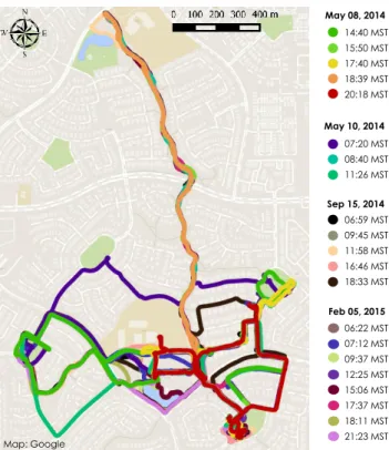
2.1 A simplified workflow for mobile measurements: From observa-tion to conclusion. . . 22 2.2 Location of the study area (background image: Google Earth). . 28 2.3 Measurement platform and sensor setup. . . 29 2.4 Transect runs in Power Ranch (background map: Google). . . . 31 2.5 The graphical user interface. (a) The Map View. Plan-view

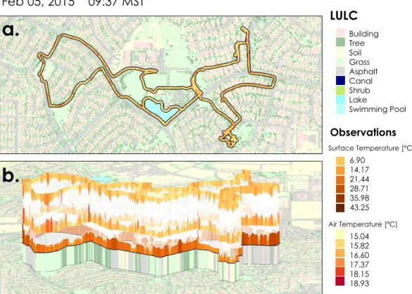
overlay of a transect on the LULC layer, visualizing a segmen-tation result (see also Section 2.6.4; background map: [46]). (b) The Fraction Plot, showing the LULC fractions within the sur-face temperature infrared radiometer’s field of view. (c) The pie-chart that complements the fraction plot. (d) Classification result based on surface temperature and land use fractions in the infrared radiometer’s source area. (e) Parallel coordinates show the semantical meaning of the classes, which have been determined during the segmentation process. . . 33 2.6 The database summary functionality. . . 34 2.7 A wall as seen from (a) bird’s view, and (b) from the side (facing

north). Surface temperature, 1m air temperature, and 2 m air temperature are stacked upon each other (from bottom to top). The lowest layer shows the LULC class of the particular route nodes. Note that some relationships between 1 m and 2 m

air temperatures can be detected: The peaks in 1 m are more intensive than those in 2 m height (background map: [46]). . . . 36

tive humidity, 1 m air temperature, 2 m relative humidity, and 2 m air temperature (from bottom to top). The lowest layer shows the LULC class of the particular route nodes. Note the visual pattern of association between LULC, temperature, and humidity (background map: [46]). . . 37

2.9 The slider can be used to interactively explore the spatial con-text of the data. The source area is attached to the bottom of the slider, while the fraction plot and the pie chart underneath the map display the composition of LULC fractions within the source area. The ellipsoid exemplifies the source area for air temperature measured at a height of 1 m(background map: [46]). 40

2.10 (a) The cluster interface, which is linked to the main window depicted in Figure 2.5. In the background, the weight vectors associated with the individual self-organizing map (SOM) nodes are visualized. They are colored using Sammon’s mapping [128] of the weight vectors into a 2D color space [131, 9, 160]. The bor-ders of the nodes represent each node’s cluster membership after the k-means clustering has been applied. (b) The results of Sam-mon’s mapping [128] of the neurons into a 2D space [131, 158]. The example is based on segmenting a mobile measurement run conducted on February 05, 2015, at 09:37 MST, based on surface temperature and air temperature in 1 m and 2 m height. . . 43

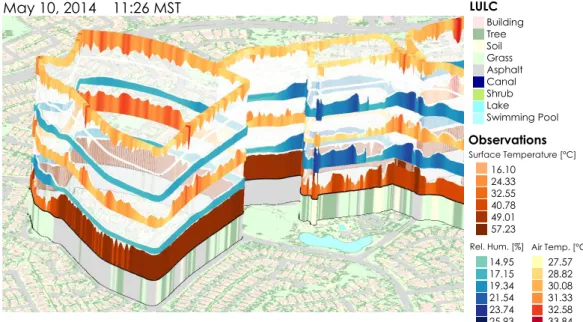
demonstrated, based on a combined SOM and k-means clus-tering algorithm [158, 161] over all measured quantities. This clustering is based purely on associations between (in order of stacking from surface) surface temperature, air temperature, and relative humidity at 1mand 2mheights a.g.l.. (a) displays the visualization of the clustering output. (b) shows the distri-bution of the cluster members along the transect route from the birds-view perspective. Note the correlations between patches of land use and cluster membership. (c) and (d) visualize the meaning of the different clusters in terms of multivariate value distribution in the map, with (c) showing the wall from the south, (d) from the north (background map: [46]). . . 46

2.12 Semantical meaning of the clusters resulting from the segmen-tation described in Section 2.7. . . 47

3.1 Time-detrended 1m FWT air temperature measurements (fil-tered and unfil(fil-tered) in the time and frequency domain. The time series was recorded on September 15, 2014, between 18:33 MST and 19:36 MST. (a) shows the time series, before and af-ter the moving average has been applied. (b) displays these time series in the frequency domain. The red line indicates the Nyquist frequency. . . 57

3.2 Upper image: Results for the parameter optimization experi-ment, averaged over all available data sets. The results cor-respond to the parameter configurations shown on the lower image: All possible combinations of varying values for the three to-be-optimized parameters have been examined. The red line indicates the best result in terms of ∆aggr. . . 59

uncorrected HC2S3 Pt100 RTD measurements, and corrected HC2S3 Pt100 RTD measurements). All time series were time-detrended prior to correction. Center: Error between filtered FWT measurements ("ground-truth") and corrected HC2S3 Pt100 RTD measurements. Bottom: The improvement of the index of agreementd, which is determined by subtractingdU N CORR,F W T from d_{CORR,F W T}. . . 61 3.4 (a) Best and (b) worst correction result from a set of 42 test

cases in terms of the improvement of d. The best and worst cases are determined by the difference of the index of agree-ment between measured and uncorrected data and d between measured and corrected data (d_{CORR,F W T} −d_{U N CORR,F W T}). All time series were time-detrended prior to correction. . . 62 3.5 Correction results. The scatter plots display the alignment of

the time-detrended and filtered FWT observations to the (a) uncorrected (but time-detrended) and (b) corrected RTD obser-vations. The 1:1 slope lines shown on both scatterplots indicate perfect alignment. Different colors correspond to different time series, in correspondence to Figure 2.4. . . 63

4.1 Overview over the user-steered workflow to visualize microenvi-ronments based on the spatial aggregation of mobile measure-ments. . . 72 4.2 Aggregating data over a regular grid (background map: [46]). . . 73 4.3 Glyph design. . . 75 4.4 An example for the glyph-based visualization of climatic

mi-croenvironments, showing a part of the covered study area. A close-up of the final glyphs is shown to the right (background map: [46]). . . 77

lead to unintuitive results. Therefore, the glyphs are compared as a whole and sector-wise. The resulting points are added up toP

P oints. . . 80 4.6 Coloring the background of each grid cell according to the

simi-larity of the glyphs associated with each grid cell. (a) An exam-ple for a case, in which the background colors of similar glpyhs become too distinct. (b) An example, where the described pro-cedure works well (background map: [46]). . . 81 4.7 Averaged parallel coordinates plot. Upper row: Averaged

par-allel coordinates for the clustered "representative" transect run.

Lower row: Averaged parallel coordinates, after all other runs have been attached to these clusters. Each averaged parallel coordinates plot represents (from left to right): Surface tem-perature, relative humidity 1 m, air temperature 1 m, relative humidity 2 m, and air temperature 2 m. Different colors repre-sent different clusters, and the dots reprerepre-sent the average value of all members belonging to this cluster. . . 84 4.8 Validation results in terms of the index of agreement (d) and

the mean absolute error (M AE). . . 86 4.9 a. Brushed parallel coordinates plots to visualize the meaning

of the clusters. b. The glyphs combining the entire set of mobile transect measurements on a map (background map: [46]). . . . 87 4.10 Coloring the background of the grid cells to highlight potential

climatic microenvironments in the study area (background map: [46]). . . 88 5.1 Steps in the method from a set of static images to a visual

summary of the temporal feature development. . . 99 5.2 a) Edge detection of significant thermal-radiative features in a

TIR image using the Canny edge detector. b) Corresponding digital photograph (provided for context) . . . 101

initial polygon, and c) converged snake. For the corresponding digital photograph, see Figure 5.2b. . . 104 5.4 If the time difference between two subsequent TIR images is very

large, the snake may converge erroneously. The images on a) have been collected at 8:17 CEST, while those on b) were taken at 10:01 CEST. Digital photographs are provided for context. . 105 5.5 A directed graph is used to visually summarize the temporal

behavior of thermal features over time. Each vertex corresponds to one thermal feature identified in the respective frame. The color for the inner circle of each vertex encodes the average temperature for the thermal feature it represents. The outer circle’s color is used to visualize the standard deviation of the measured temperatures within this feature. Finally, the size of each vertex represents the thermal feature’s size in the image. . 106 5.6 The graphical user interface. . . 108 5.7 The edges of the shade were fragmented, but could still be

rec-ognized. . . 113 5.8 The graph that corresponds to the delineation of the surface

area underneath the tree’s canopy, corresponding to the image series in Figure 5.9. The graph represents the diurnal curse of the surface temperatures (times of day were added to the image for clarity, they are not generated by the tool). . . 114 5.9 The image series, on which the graph in Figure 5.8 is based

(times of day were added to the image for clarity, they are not generated by the tool). The translation between the images becomes large, which does not make an animation reasonable. . 115 5.10 Even on ultra-low-resolution images, features can be delineated

using snakes and GVF [85, 172], if they are salient enough. (a) shows the initial polygon, and (b) the converged snake. The image has a resolution of 60x60 pixels. . . 116

green). . . 120 6.2 A combined visualization example (created with IES-VE):

Iso-surfaces for air temperature (gridded Iso-surfaces), cutting planes with color-coded vector glyphs for air flow and contour lines for wind speed, and tracked particles. . . 127 6.3 Isosurfaces for air temperature (created with IES-VE). . . 129

2.1 Reference weather during the mobile measurements, averaged over the time span in which all measurements of a day took place (reference meteorology from MesoWest 2014 [105]: Cloud cover from KIWA Phoenix-Mesa Gateway, temperature and wind data is the average of the data from four nearby stations surround-ing the study site, i.e. AU340 Gilbert, D2495 Gilbert, AT202 Gilbert, and SRP31 Rittenhouse). . . 32 3.1 Comparison of the spatial resolution at three different movement

speeds, given by the time constants of different sensors. . . 65 4.1 Metric applied for glyph comparison. . . 78 4.2 Experimental setup for the quantitative sensitivity analysis. . . 82 6.1 Capabilities of DesignBuilder / IES-VE as opposed to the

re-quirements resulting from an architectural workflow. . . 128

Introduction

1.1

Motivation

Cities are one of the major alterations of a natural landscape, transforming structural and geometrical components as well as the predominant land cover through buildings and impervious surfaces [114, 148, 155]. In addition to that, the inhabitants of a city release heat, moisture and pollutants through their activities [148, 155]. As a result, urban areas show a modification of radiative, thermal, moisture and wind flow characteristics when compared to their sur-rounding rural landscapes [114].

The discipline of urban climatology investigates these alterations, as well as their effect on the city dwellers [115]. The atmospheric processes related to the modifications induced by urban areas occur at different spatial scales, vertically as well as horizontally [115] (see Section 1.2.1). In this context, the urban microscale considers the atmospheric impact of surface material patches, single trees, or small-scale building and landscape configurations, all of which are important to describe the climate within the urban canopy layer, i.e. the area between ground and roof-level [113, 114].

The urban microscale is in the focus of the research activities of my collab-oration partners at the Arizona State University (ASU) in Tempe, Arizona, USA. They analyze the physical microclimate dynamics across space and time and in dependency of urban form and design, using a variety of data modal-ities. The latter range from in-situ measurements within physically available neighborhoods to the simulation of microclimate variability induced by

thetical urban form and landscaping scenarios [107].

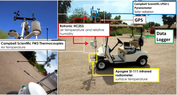
In the context of in-situ measurements, time-varying thermography with a hand-held infrared camera is utilized point-wise in space to gain an overview over the thermo-radiative environment induced by urban features such as trees. Besides, mobile transect measurements are conducted to investigate the ex-tent of and transition between microclimates, as well as their time-varying atmospheric characteristics. These observations are retrieved by traversing different urban design configurations using a sensor platform attached to a golf cart. The resulting data sets are complex and afflicted with uncertainties, which makes their analysis difficult and time-consuming using existing tools and methods.

Motivated by the resulting domain-specific problems and as an attempt to support the described research activities, my dissertation is dedicated to the investigation of appropriate visualization and analysis techniques that can help to increase the insight into the the described in-situ observations. Providing an interactive means to explore these data sets can increase the knowledge about predominant physical interrelations between the investigated objects.

1.2

Background

1.2.1

Urban microclimate research

The importance of scale in urban climatology: Basic definitions The main objective of urban climatology is the investigation of the interac-tions between the built environment and the atmosphere [115]. It operates on different spatial scales, vertically as well as horizontally [115].

In the vertical dimension, Oke [114, 113, 115] distinguishes between the

Urban Canopy Layer (UCL), which ranges from ground to roof-level, the

Roughness Sublayer (RSL), which ranges from ground to approximately 1.5 to 4-times the roof-level height, and theUrban Boundary Layer (UBL), which extends up to that height, in which the vertical atmospheric effect of the urban landscape is not noticeable anymore. The atmospheric processes in the lowest layer, the UCL, are governed by the microclimatic effects induced by individ-ual three-dimensional urban objects, e.g. buildings or trees. The individindivid-ual

impact of these features is blended at the upper border of the RSL, which is in turn dependent on a variety of synoptic and geometrical factors. Finally, the atmospheric properties above the RSL up to the upper border of the UBL are dominated by the averaged local to meso-scale impact of the "urban surface" with its characteristic roughness, thermal and moisture properties [114, 113].

In the horizontal dimension, the impacts of the urban landscape onto the atmosphere can be observed at the micro-, local, or mesoscale [113, 115]. The

microscale ranges from less than one meter to hundreds of meters, depend-ing on the size and configuration of individual builddepend-ings, yards, streets, small parks, or trees [113]. Consequently, the impact of these urban design ele-ments onto the properties of the immediate atmosperic surroundings can best be observed at this scale. The combination of different microscale processes, generalized to individual "microclimates", determine the atmospheric proper-ties and their spatial variability within the UCL [114]. The local scale ranges roughly from one to several kilometers, depending on the extent of more or less homogeneous building and landscape configurations [113, 148]. Observing the urban climate at a local scale means that the atmospheric impacts of entire neighborhoods or city districts are considered, averaging out the microscale im-pacts of the individual urban objects within these areas [113]. The mesoscale

corresponds to the scale of an entire city and its surroundings, at an extent of several to tens of kilometers [113, 115]. At this scale, the atmospheric impact of the city as a whole as compared to its rural hinterlands can be investigated. It has to be noted that the described scales should not be seen as strict par-titions, but that they rather appear as merged within a continuum [114]. Nev-ertheless, as Arnfield [13] states, they constitute the morphological units based on which atmospheric processes are investigated and described, whereas scales with a larger spatial extent hierarchically aggregate all complex processes at scales with a lower spatial extent. This aggregation also results in a decreasing variability of radiative, thermal, moisture, or wind flow patterns [13]. Thus, as a result, the local climate regimes of two adjacent neighborhoods will be less distinct from each other than the microclimates induced by a grass patch with trees versus an adjacent open space with asphalt surface occuring within these neighborhoods [13].

Investigating the urban microclimate: Topics, goals, and data modal-ities

Although the general topic of urban climatology can be described as the study of the interrelations between the built environment and its surrounding atmo-sphere [115], the subtopics are many and various. They can roughly be par-titioned according to the concept of horizontal and vertical scales described in Section 1.2.1. Since my dissertation focuses on visualization and analysis techniques for the urban microclimate, the topics, methods, and challenges of research activities operating within the UCL and at the microscale are briefly outlined in this Section, without claim for completeness.

In terms of the thermal regime within the UCL, the spatio-temporal char-acteristics of the canopy layer urban heat island (UHI) is one of the most extensively studied effects [147, 143, 13, 148]. In its most general terms, the UHI can be defined as the thermal difference between an urban area and its rural hinterland, whereas the temperatures within the city center are warmer than those in the city’s surroundings [114]. The UHI intensity varies over time, and reaches its maximum during the night [75]. At daytime, shading effects induced by high-rise buildings can even reverse the effect [114, 84, 107].

Although the UHI is obviously only recognizable at the mesoscale, the canopy layer UHI is the result of the combined effects of different urban mi-croclimates, as induced by an urban canyon. The urban canyon consists of adjacent houses and the space between these houses, and it can in simpli-fied terms be seen as the principal unit of the urban canopy layer [114]. The distribution of radiative fluxes occuring within these units are dependent on their geometric properties [143], and the combination of the latter with differ-ent kinds of surface materials, vegetation cover, and anthropogenic activities determine the individual climatic behavior of an urban canyon in terms of moisture, air flow, air quality and temperature [114, 109].

The detailed investigation of these effects, either separate or combined, is in the focus of urban microclimatology. On a theoretical basis, the general physical processes governing the exchange of heat and moisture between the different surface elements are studied, as well as the airflow around these three-dimensional obstacles [143]. Increasing the knowledge about these processes leads to improved computational models that can be used for a variety of

ap-plications [32].

The most important application of urban microclimatology is optimiza-tion of urban design to create sustainable, comfortable, and therefore livable cities [108, 23]. For example, investigating the airflow regime within an urban canopy can help to determine pedestrian comfort, while the combined effects of urban canopy and urban boundary layer can help to predict the disper-sion of pollutants [143]. Predicting the combined impact of urban form and landscaping onto radiative, thermal, moisture, and airflow conditions within the urban canopy layer can assist the design of thermally comfortable outdoor spaces, ameliorating the effects of climate change [108, 23]. Well-chosen build-ing parameters (material, orientation, geometric design) can lead to a lower energy consumption through a decreased necessity of air condition or heating, and thus to a more sustainable urban development [108].

The data modalities used to achieve the described goals can roughly be partitioned into three groups: In-situ measurements of atmospheric variables, remote sensing, and simulation.

In-situ measurements are conducted using weather stations at fixed spatial locations within an urban area. Usually, these weather stations are placed at sites that are considered representative for the local climate within a more or less homogeneous neighborhood, without capturing the signal of individual urban features [109, 113, 148]. Currently only a few examples for stationary sensor networks measuring the urban microclimate exist [109]. Frequently, these measurements are conducted using small or hand-held devices which are then placed at the investigated site. In this context, thermal infrared im-agery using hand-held devices can be used to complement these observations. However, wireless technology or low-cost miniature sensors are considered to increase the number of stationary microclimate measurement sites [109].

Obviously, stationary measurements can only be conducted pointwise in space. In contrast, mobile measurements using moving sensor platforms are a possibility to increase the spatial coverage of observations, enabling the investi-gation of the spatial variability of the urban microclimate at a high resolution (see, e.g., [73]). In a less controlled way, data crowdsourcing through novel mobile sensor technologies is increasingly used to not only measure the atmo-spheric state at covered locations, but to also investigate its impact on the

activities of the participating people [32].

In addition to the described methods to obtain in-situ measurements, re-mote sensing data are another key data modality. For example, the geometries extracted from LIDAR data sets can help to analyze small-scale radiation en-vironments using measures such as the sky-view-factor [143]. Besides purely geometric information, detailed land cover / land use (LULC) maps are de-rived from remotely sensed images, revealing the spatial distribution of urban objects and surface materials (see, e.g., [46]). This information provides valu-able information about the spatial context of in-situ measurements, but can also be used to inform simulation models, the third modality used in urban microclimate research.

1.2.2

Visualization and analysis techniques for

atmo-spheric data sets

Interactive visual exploration techniques are not commonly used so far by at-mospheric scientists, although sophisticated methods and toolkits have been developed by the visualization community [92, 111, 153]. In this context, Nocke et al. [111], Tominski et al. [153] as well as Ladstädter et al. [92] state that the visualization techniques used by atmopheric researchers are frequently restricted to standard techniques, including 2D diagrams such as time series graphs or scatterplots, or colored 2D maps. These (static or animated) vi-sualizations are typically created using statistical toolkits such as MS Excel, R, or Matlab, or general purpose geographic information systems such as Ar-cGIS [112, 111], an observation I also made during my collaboration with urban microclimate researchers at the Arizona State University. While the resulting plots are easily understandable, they are frequently restricted to summarizing time series or scatterplots without including the spatial context in the case of 2D diagrams, or showing only one variable per image in case of spatial plots [111, 92]. This aggravates the combined visual exploration of the tem-poral development of investigated atmospheric parameters, their multivariate relationships, and their relation to the spatial context [111]. Thus, interesting features or patterns in the data might remain undetected [111, 92].

On the other hand, a large variety of sophisticated interactive visualization techniques for atmospheric data sets have been developed over the years, es-pecially for global and regional scale data sets stemming from observations, remote sensing, and simulations. Application areas range from multivariate exploration of time-varying uni-modal data sets [92, 149] to the integration of observation and simulation data for verification purposes, either qualita-tively [71] or quantitaqualita-tively [163], to uncertainty visualization in climate and weather models [130]. Ladstädter et al. [92] demonstrate that visual explo-ration techniques can help to provide holistic views of the investigated climate data sets, which facilitates building hypotheses about the data. In their highly interactive tool SimVis, they incorporated techniques including interactive fea-ture selection, brushing and linking, focus and context, and flexible (algebraic) combination of variables. Enabling scientists to find unexpected features or patterns, such techniques can complement more quantitative statistical anal-yses, for which, in many cases, a hypothesis is needed beforehand [92]. Helbig et al. [71] use a variety of mapping techniques to combine several data fields in one view, through which users can navigate either on a desktop computer or in a virtual reality environment. Integrating data sets from both simulation and observation data, they also support the qualitative validation of simula-tion results. Nocke et al. [111] created a library for a suite of visualizasimula-tion techniques that can be used for several analysis purposes related to climate simulation data, using both visualization techniques that are typical for the atmospheric sciences, but also innovative approaches. Tominski et al. [153] visualize global and regional climate networks within their spatial reference frame, encoding important network information using the vertices of the re-sulting graph and enabling data filtering to reduce visual clutter.

While there has been advancement in visualizing larger scale weather and climate data sets, examples for the visualization and analysis of urban (mi-cro)climate data sets are rare, as also stated by Röber et al. [125]. However, several examples can be found for the visualization of urban microclimate sim-ulations. In this context, Röber et al. [125] use Avizo Green to visualize inner city ventilation, and interactions between an individual building and its en-vironment. Heuveline et al. [74] explore the utilization of augmented reality techniques to visualize airflow around building structures. A more integrated

approach was chosen by Wang et al. [162]. Not only limited to urban areas, the authors combine a microscale meteorological model with Google Maps / Google Earth to facilitate the manual initialization of the model in terms of the three-dimensional objects within the domain and the final visualization of the simulation results, using standard mapping techniques. The authors also demonstrate how Google Maps / Earth can be used to map observation data sets.

Even more rare are visualizations of observation data sets in an urban cli-mate context. There are some examples for the visualization of air quality data sets, which are obviously not necessarily bound to an urban context. For example, Qu et al. [120] developed a visual analytics system for station-ary air pollution measurements from Hong Kong. In their tool, they combine several visualization techniques, including a circular pixel bar chart, a par-allel coordinates plot with an s-shaped axis to encode wind direction, and a complete weighted graph showing pairwise correlations between measured at-tributes. Their system, however, does not include the spatial context of the measurement stations. Also dedicated to air quality data, Liao et al. [97] implemented a web-based air quality analysis system for stationary measure-ments that comprises a map view with pie-charts encoding the distribution of certain air quality indices over a selected time interval, a parallel coordinates plot, and a time-series plot.

Recently, with the advent of mobile sensing and data crowdsourcing, a va-riety of web-based visualization tools have been developed that either attempt to inform the general public about the collected data sets in their city (see, e.g., [168]), or that are rather designed as a data storage, management, and display systems [87]. While providing interactive navigation of the data sets, these systems are usually limited to standard mapping techniques and do not provide multivariate exploration facilities.

1.3

Contribution

In summary, the contribution of this dissertation is the application and adap-tation of visualization and exploration concepts to enhance the analysis of

important urban microclimate data modalities. The investigated approaches go beyond standard mapping techniques that are currently used in domain-specific research. Providing additional views on the complex patterns inher-ent in observations, the suggested techniques attempt to facilite data-driven reasoning about the relationships between urban form and the atmospheric environment it induces.

The main focus lies on the interactive visualization of data sets resulting from mobile measurements, which can be seen as one of the most complex modes of in-situ observations due to their spatio-temporal dependence, their multivariate nature, and the various error sources associated with a moving platform. Combining concepts from both visual analytics and atmospheric sciences, a prototypic tool is developed that assists urban microclimate re-searchers not only to explore their measurements in detail and with the ex-plicit consideration of a sensor’s spatial context [60], but also to search for multivariate patterns that can finally lead to the delineation of climatic mi-croenvironments within a study site [61].

Within the prototype, a suite of data preprocessing techniques enables the researchers to quickly increase the reliability of their observations and to in-tegrate them with other data sources, including high-resolution land cover maps and measurements from surrounding weather stations. In this context, research was also directed into evaluating and improving domain-specific tech-niques for sensor lag correction, which can enhance the spatial resolution of mobile measurements taken with a slow air temperature sensor [63].

Besides providing interactive data exploration tool for mobile transect mea-surements, a smaller project within this dissertation deals with another in-situ observation mode used in urban microclimatology: Thermal infrared imagery with a hand-held device. Observations are conducted to gain a spatial overview of the thermo-radiative environment at a study site, but also to investigate the time-varying progression of specific thermal features. Images recorded with hand-held devices can pose the challenge of varying perspective onto the in-vestigated object, making the manual feature extraction necessary. Motivated by these challenges, a tool was implemented to assist accurate feature extrac-tion and to visually summarize the results of the extracextrac-tion results, combining well-known image processing and visualization techniques [58].

Finally, going beyond the visualization of the outdoor urban microclimate, currently used visualization techniques in building performance simulation re-sults are evaluated using feedback from an architect [64]. The findings from this study were the starting point for a larger project aiming at the extension of existing exploration techniques.

1.4

Collaborations

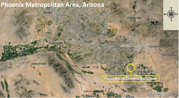
Most of the projects described in this dissertation originated from active in-volvement in urban microclimate research at the Arizona State University (ASU) in Tempe, Arizona, USA. Main collaborators were Research Assistant Professor Dr. Ariane Middel (School of Geographical Sciences & Urban Plan-ning and School of Sustainability, ASU), Assistant Professor Dr. Benjamin L. Ruddell (Fulton Schools of Engineering, ASU), and Prof. em. Dr. An-thony J. Brazel (School of Geographical Sciences & Urban Planning, ASU). The central theme of their research activities is the impact of urban design and landscaping on the surrounding microclimate. In particular, they inves-tigate the spatio-temporal physical dynamics of microclimate in a desert city and their influence on thermal comfort and perceptions. For their research, they use in-situ measurements recorded using a sensor platform attached to a golf-cart, which is then moved through selected study sites located in the Phoenix Metropolitan Area, Arizona. Hand-held thermographic images are used to capture the impact of tree-shade on the spatial distribution of surface temperatures. While both thermographic images and mobile measurements help to examine current climatic conditions in a certain, physically available neighborhood, simulation data sets are created and analyzed to investigate a number of hypothetical urban form and landscaping scenarios in a structured way [107].

Furthermore, the tool described in Chapter 5 was implemented in collabo-ration with Lars Hüttenberger and Nils H. Feige.

The research described in Chapter 6 was conducted in collaboration with an architect, Eva Hagen, as well as with M.Sc. Diana Fernández Prieto, Dr. Daniel Engel, and M.Sc. Stephanie Schweitzer, at that time members of the Computer Graphics and HCI Group, Department of Computer Science,

University of Kaiserslautern. Furthermore, Dr. Inga Scheler (RHRK Kaiser-slautern), and Michael Böttinger (Climate Computing Center, Hamburg) are part of this project, which is still on-going.

1.5

Structure of the dissertation

The main contribution of this dissertation is the prototypic implementation of a visualization and analysis tool for mobile urban microclimate data sets. Therefore, three chapters of this dissertation (Chapter 2 through Chapter 4) are dedicated to this topic. Chapter 2 provides an overview of the research background, data set characteristics, the framework components, and its use case for the detailed analysis of one single mobile measurement run. In Chap-ter 3, an improved method to correct air temperature measurements for sensor lags is portrayed, before Chapter 4 explains, how the visual delineation of cli-matic microenvironments can be facilitated based on the spatial aggregation of a set of mobile transect measurements.

A smaller project within this thesis focuses on the analysis of thermal in-frared images for urban microclimate research. In this context, Chapter 5 describes a prototypic tool that assists the analysis of a set of time-varying thermographs.

Chapter 6 focuses on the visualization of relationships between architectural design and microclimate. In particular, the state of the art of the visualiza-tion in current building performance simulavisualiza-tion tools is described based on a literature review and feedback from an architect.

TraVis – A Protoypic Software

for the Visualization and

Analysis of Mobile Urban

Microclimate Measurements

This chapter introduces the main project of this dissertation: The implementa-tion of TraVis, a prototypic visualizaimplementa-tion tool for the analysis of mobile transect measurements in an urban microclimate context. TraVis is designed to support the workflow of analyzing mobile measurements by providing functionalities for data preprocessing, data representation, and data analysis. The framework complements domain-specific state-of-the-art visualization techniques, which mainly use standard mapping and timeline plots, by incorporating spatial context and multivariate relationships into the (visual) analysis. I developed TraVis in close collaboration with two urban climatologists (Ariane Middel and Benjamin L. Ruddell), who use mobile transect measurements to observe the impact of the build environment on microclimate in a desert city. They continuously evaluated the design decisions, and gave important advice about domain-specific analysis techniques.

While this chapter provides an overview of the background of the described research, the sample data set with which it was developed, and the basic sys-tem components of the tool, the following chapters describe work that extend the core visualization and analysis functionalities. In this context, Chapter 3

introduces an improved method for sensor lag correction, which is an important preprocessing step for mobile measurements conducted with slow sensors. Fi-nally, Chapter 4 describes a purely data-driven approach for the identification of climatic microenvironments, which can handle diverse mobile measurement routes and spatial data-sparsety.

To a large part, this chapter is based on a peer-reviewed full-paper, which was published in the proceedings of PacificVis 2015 [60]. The description of the data set is taken from a paper that I recently submitted to Urban Climate [63].

2.1

Introduction

Mobile transect measurements are an important tool for urban climatology. A sensor platform is mounted to a vehicle, which is then moved along a predeter-mined, potentially interesting route in order to investigate the spatial variation of observed parameters. In contrast to stationary measurements, which are collected only pointwise in space, mobile measurements deliver high-resolution spatial data along a line. This is useful to examine the extend and properties of contiguous areas of similar climate, as well as the transition between them. Relating these patterns to the surrounding urban form can inform the design of sustainable and comfortable urban neighborhoods [108].

Data sets from mobile measurements are multivariate and (often-times) time-varying trajectory data. A trajectory is defined as a time-ordered se-quence of spatial locations visited by an entity [7, 8, 154, 124]. Mobile measure-ments build on these two elementary components, although sensors mounted on the moving platform add additional environmental attributes, such as air temperature, surface temperature, relative humidity, short- and longwave ra-diation or air quality data, varying dynamically along the transect route. The time-varying component of the data set is introduced by repeating the tran-sect measurements periodically. Furthermore, each sensor and therefore each trajectory attribute has a unique and dynamically varying spatial context and representative source area corresponding to the observation.

In this Chapter, I introduce a framework for the visualization and analysis of these complex movement data sets. It is structured as follows: The domain-specific background of this work is described in Section 2.2, leading to the goals

and contribution to the urban climate as well as the visualization community in Section 2.3. Related work, as seen from a visualization point-of-view, is por-trayed in Section 2.4. Section 2.5 provides details on the data set, which was used for implementation and testing of the prototype. The main components of the framework are shown in Section 2.6, while Section 2.7 demonstrates, how they can be used to analyze a single mobile measurement run in detail. Finally, a conclusion is provided in Section 2.8.

2.2

Mobile measurements in urban

climatol-ogy

2.2.1

State of the art

Mobile Measurements

Mobile transect measurements are frequently applied in urban climatology to investigate the spatial and temporal dynamics of atmospheric conditions within the urban canopy layer, i.e. in the space between ground and roof level. Several phenomena can be investigated using this technique. Research usually focuses on either the more general impact of urban form on microclimate [146, 22] or on the analysis of specific climatic phenomena, such as the urban heat island [73, 141, 110, 150] or park cool islands [33]. Studies also investigate health implications of the urban environment, e.g. through air quality measurements [45, 65] or through the analysis of thermal comfort [156].

Mobile transect observations frequently include air temperature and rela-tive humidity [33, 141, 73, 156]. Depending on the research goal of the study, additional variables are derived from these observations, e.g., the dew point temperature [146, 150], or measured. For example, Vanos et al. [156] ob-serve total incoming shortwave radiation to investigate the moderating effect of parks onto the human energy budget. In urban areas, air quality observa-tions are also an important source of information. Thus, flexible measurement systems have been developed and used for mobile air quality measurements. The Aeroflex bike [45] is a notable example for this application.

some cases, the behavior of the observations with increasing height above the surface is an integral part of the research question. For example, Chow et al. [33] used mobile measurements at four heights to derive temperature profiles over a variety of surface types to investigate the characteristics of the noc-turnal park cool island effect on the Arizona State University (ASU) campus in Tempe, Arizona. Land use / land cover (LULC) surrounding the sensors is frequently included into the analysis, using various methods. Sun et al. [150] relate their observations to the normalized differenced vegetation index (NDVI) within two constant radii around the sensor locations. Heusinkveld et al. [73] use the fraction of buildings, water, and vegetation to statistically analyze the relationship between observations and urban landscape context.

Recently, larger measurement campaigns have been launched that inves-tigate the urban climate by using sensors mounted to public transportation vehicles. These projects cover a larger area, and thus allow the analysis of the urban climate at the city-scale and with a high temporal resolution and regu-larity. Buttstädt et al. [24] use air temperature and GPS loggers attached to busses to increase the spatio-temporal coverage of air temperature data for the city of Aachen, Germany. The same team developed a prototypic multi-sensor measurement device in the URBMOBI project [88, 127], which measures air temperature, relative humidity, and solar radiation. It can also be attached to vehicles moving through a city, monitoring data to inform models [127], or to identify (un-)comfortable areas within a city [88]. The German Weather Service (DWD) mounted air temperature and relative humidity sensors to streetcars to retrieve information about spatio-temporal dynamics of the air temperature distribution in Halle, Germany, which in turn complements data retrieved from stationary measurements and simulation models [41]. While the named examples focus on the observation of the urban heat island or try to derive implications about the thermal comfort of city dwellers, other larger measurement campaigns systematically acquire data about air quality. The AERO-TRAM project [65] is one of these attempts: Here, sensors are attached to streetcars, and data along two different routes are collected continuously. Similarly, Hasenfratzet al.[70] equipped ten streetcars in Zurich, Switzerland, with observation systems for ultra-fine particles. Using these data, they devel-opped a regression model that eventually results in a city-scale air pollution

map.

Visualization

In the urban climate literature, mobile transects are frequently displayed as two-dimensional plots with the spatial location on the x-axis and the observed quantities on the y-axis [150, 156, 65]. Sometimes, the x-axis is complemented by LULC information located directly under the sensor platform to facilitate the relation of measurements to spatial context [22, 146]. Another frequently used visualization is a two-dimensional spatial plot of transect measurements on a map [73, 33, 45], displaying only one variable, one measurement height, or one point in time. In TraVis, I combine the advantages of these visualization methods, displaying a user-defined number of variables as stacked ribbons on a background map, and transferring the generally two-dimensional diagrams into their native spatial context.

Recently developed measurement systems, such as URBMOBI [88, 127] or the Aeroflex bike [45], include their own automated processing and visualiza-tion pipelines. In the URBMOBI system, collected and processed data are fed into simulation models, the results of which can then be explored along with the transect measurements using the MEA user interface [106, 88, 127]. This interface provides a data integration facility, which is capable of combining information from different sources and with diverging spatial resolutions, as well as standard visualization techniques to explore the data. Thus, a user can choose an area of interest (AOI), and display the distribution of several vari-ables within the AOI using side-by-side images. Furthermore, MEA allows the extraction of time series for individual locations, which are then displayed in a standard time-series plot [106]. For the Aeroflex bike, Elenet al.[45] developed a fixed data processing pipeline. The raw data collected during single runs can be visualized using a quick mapping interface called VITO SensorView, which allows plotting one variable at a time simultaneously on a map and in a time-series diagram, limited to this single run [159]. After that, the data runs through an automated data preprocessing chain, before it can be visualized using a web-based interface based on a GeoServer and Google Earth plug-in. This map is updated after completion of additional measurement runs, while repeated runs – which are conducted along the same route and at fixed points

in time – are displayed on the map using summary statistics [45]. Another ex-ample is Vizzly [87], a data storage and aggregation tool that maps aggregated measurements from both mobile and stationary sensors in a timeline plot and on a map. The tool enables interactive browsing for very large sensor data sets at different spatial and temporal resolutions, and was, e.g., used for a larger air quality measurement campaign using sensors on public transportation ve-hicles in Zurich, Switzerland [70]. Boufidou et al. [21] developed a database that is meant to facilitate the management of urban climate data sets. It can manage geometrical and material information related to the urban landscape, as well as mobile air temperature measurements that have been collected with an Arduino platform.

In contrast to the mentioned data management and visualization tools, TraVis was developed with a focus on the visualization and analysis of mobile measurement data collected during smaller campaigns. Using visualization research, the prototype enhances standard mapping techniques to provide de-tailed views on the multivariate and complex nature of mobile transects at the microscale.

2.2.2

Data set characteristics

Mobile transect measurements are multivariate geospatial movement data. Us-ing the notation described in [3, 154], the latter comprise a set of spatial loca-tions per trajectory,S={s0, ..., sn}, and a time stamp ti associated with each element of S, yielding T ={t0, ..., tn}, with n >0 and indicating the number of sampled positions. Using T and S, further sets of dynamically changing attributes A0,...,m can be computed per location and time stamp, including movement direction, velocity, and acceleration [8, 154]. Similar to the data sets visualized in [154], mobile-platform transect data sets involve additional, dynamically changing attributes Am,...,n complementing S and T, such as air temperature, relative humidity, or surface temperature.

In addition to these properties, mobile transect measurements feature two peculiarities. Firstly, the attributes collected during mobile transect measure-ments are related to a certain height above ground level (a.g.l.), which is either given by the mounting height of the sensors for in-situ measurements (e.g., air temperature) or by the location of the investigated object for remotely sensed

data (e.g., surface temperature). This information is an important aspect dur-ing data analysis. It complements the 3D spatial locations of a movdur-ing entity’s path in conventional trajectory data sets, which is commonly described by a set of 3D geographic coordinates (latitude, longitude, and elevation above mean sea level (a.s.l.)). Since the set of spatial locations is usually displayed on a two-dimensional map that represents the projection of the Earth’s surface onto a plane, the measurement height a.g.l. introduces a vertical offset dimension in addition to the resulting set of two-dimensional coordinates on that plane. Secondly, the analysis of the spatial context of the data differs from usual trajectory data sets. In conventional trajectory data sets, the spatial context is analyzed to facilitate reasoning about certain movement patterns. For mo-bile transect measurements, the trajectory is exogenously fixed based on the aim to observe relationships between multiple environmental attributes and the spatial context, utilizing spatial context to explain attributes rather than the trajectory itself. The multiple sensors in a research transect each measure a different field of view, and as such each of multiple attribute observations has a distinct and separate relationship to the spatial context.

2.2.3

Challenges during data analysis

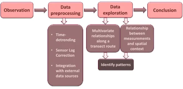
The specific tasks during the analysis of mobile measurements depend on a central research question that is individual for each study. Nevertheless, uni-versal tasks could be identified by the collaborators of this research, Ariane Middel and Benjamin L. Ruddell, which are also mirrored in the literature. To summarize these findings, a very general workflow is depicted in Figure 2.1.

After observation, climatologists need to preprocess mobile observations to establish precise measurements of attributes and exact relations to their spatial context. For example, this includes a time-detrending step to filter out potential impacts of changing reference weather during the course of a run [147]. This way, the variability of the attributes along a route can more reliably be traced back to the surrounding urban form and landscape. Fur-thermore, sensor inertia has to be taken into account. If the sensors are too slow to synchronize their readings with the conditions of the traversed mi-croenvironments, the spatial resolution of the observations will be reduced. This error source can be avoided either through correction (see, e.g., [1]) or

Observation Data preprocessing Data exploration Conclusion Relationship between measurements and spatial context Multivariate relationships along a transect route Identify patterns • Time-detrending • Sensor Lag Correction • Integration with external data sources

Figure 2.1: A simplified workflow for mobile measurements: From observation to conclusion.

through adapting the number of and distance between measurement points to the spatial resolution dictated by the sensor’s inertia [24].

Besides these data-immanent correction procedures, the observations also need to be integrated with external data sources that complement the informa-tion provided by the mobile measurements. This informainforma-tion can, e.g., consist of maps, revealing the spatial context of the traversed route. Also data from stationary observations can be useful either as a base for comparisons with mobile measurements (e.g., [24]) or to retrieve additional information about the weather conditions during a measurement run (e.g., [150]).

After preprocessing, the data can be analyzed in terms of the individual research goal. However, a common goal of mobile measurements is the inves-tigation of the spatial variability of observed attributes (because otherwise, stationary measurement would suffice), and to explore the reasons for this variability (e.g. in terms of a varying landscape). Patterns identified during exploration can then lead to a conclusion.

2.3

Research goals and contribution

The overarching goal of this project is the development of a tool that assists urban microclimate researchers during data preparation, transformation, ex-ploration, and analysis of the relationship between multiple mobile platform observations and spatial context. As such, this research contributes to both the discipline of urban climatology and visualization.

2.3.1

Contribution to the urban climate community

The contribution of this project to the urban climate community is an interac-tive visualization and analysis tool, which enables researchers to explore their mobile measurements in detail, to put it into relation with the spatial context, and to detect potentially relevant patterns in the data based on clustering and aggregation techniques. To the best of my knowledge, to date no tool exists for the comprehensive analysis of the collected data, although mobile transect measurements are a common observation technique in urban climatology.

While the tool includes standard preprocessing techniques such as time-detrending, research has also been directed towards the evaluation and im-provement of existing approaches for sensor lag correction (compare Chap-ter 3). The stacking-based visualization approach combines the advantages of the frequently used uni-variate geospatial mapping with the evenly frequently used multivariate x-y-diagrams, enabling the simultaneous inspection of a set of measured attributes in their spatial context. At the same time, the esti-mated sensor-specific source area can be used to relate the measurements to the land cover fractions that theoretically impact them. Finally, I implemented a visualization technique for spatially aggregated mobile measurements that integrates data from diverging traverse routes. The visualization does not just use simple aggregation measures, but it provides a detailed representation of urban microenvironments, their characteristics, their extends, and transitions between them.

2.3.2

Contribution to the visualization community

From a visualization perspective, this project adds to the research field of geospatial trajectory visualization: I developed an interactive visualization for

multivariate trajectory attribute data, providing a detailed view of their dy-namic behavior during a mobile transect measurement run. In addition, the dynamic spatial context is not limited to visualizing a background-map, but its impact onto the trajectory attributes can interactively be explored employing the meteorological concept of a source area, which is a notion for the spatial field of view of this class of sensors [136]. An interactive clustering interface enables the user to classify transect segments according to coherent patterns of multivariate relationships either between atmospheric attributes alone, or between atmospheric attributes and their associated land use fractions within the sensor-specific source area. Finally, a glyph-based visualization technique for aggregated multivariate trajectory data was developed and added to the framework (Chapter 4). As a result, the prototype comprises capabilities to qualitatively and quantitatively explore spatial and multivariate interdepen-dencies within the data set under investigation, and structures the underlying space according to what has been measured on top of it.

2.4

Related work

Since mobile transect data sets share several characteristics with conventional trajectory data sets, the related work for this research mainly consists of visual analytics for movement data, which will be described in this subsection.

During the last decades, research has been conducted on the visualization of and interaction with large geospatial trajectory data sets. Standard tra-jectory data sets are multidimensional, and include space, time, and other attributes associated with movement (speed, direction, acceleration), moving entities (age, gender, vessel type), or – as in the case considered for this re-search – contextual environmental attributes that change over the course of a trajectory [160]. Depending on the research goal and the underlying applica-tion scenario, studies concentrate on one or more of these dimensions.

Studies focusing on the spatial dimension of movement data frequently clus-ter, filclus-ter, or aggregate trajectories to facilitate reasoning about explanatory

patterns. Rinzivillo et al. [124] apply progressive clustering to a data set describing car movement in Milan, where simple distance functions based on start, destination, a set of waypoints, temporal distances between those points or a combination of these aspects can be used successively. Andrienko et al.

[6] describe an iterative clustering approach on a trajectory data set, which relies on the initial definition of a "classifier" resulting from clustering a subset of the data set. This classifier is then applied to the remaining data, while it can also be interactively refined if necessary. Andrienko and Andrienko [7] use accumulations of significant points on trajectories (starting points, desti-nations, stops, turns) to partition the underlying space. Movement occurring between these areas is aggregated and visualized using a flow map. Krügeret al. [91] developed "TrajectoryLenses", an intuitive spatial filter interface for a large trajectory data set. Using three different kinds of TrajectoryLenses, a user can investigate the set of trajectories with common starting points, end points, intermediate route points, or a combination of these. A temporal filter can also be applied to the data by selecting an interval on a hierarchical time slider.

In addition, studies include spatial semantics and a visualization of how trajectory patterns change over time. One example is described by Krüger

et al. [90], where information about places of interest in direct adjacency to the trip destinations are streamed from a location-based application called Foursquare. A time-line view reveals which places were visited when and how often. Growth ring maps were introduced by Bak et al. [17]. Whenever an entity visits a specific location, the ring around that place grows. Spatial se-mantics and temporal information are included by color-coding the rings. In a study by Wang et al. [164], spatial semantics occur as an underlying road network. Trajectory data recorded by taxis are matched with this network to investigate the spatial distribution of traffic jams in Beijing, and the result is visualized as a 2D map. The average speed of the taxis is encoded as addi-tional attribute through color-coding. A time-line view shows the temporal distribution of the traffic jams, while a graph projection view displays the in-terrelations between traffic jams over space and time. Lundblad et al. [98] developed SWIM, a tool designed to help shipping companies in route plan-ning. In SWIM, the trajectories of ships are set into context with weather