Interreg Alpine Space project ‐ NEWFOR Project number 2‐3‐2‐FR
NEW technologies for a better mountain FORest timber mobilization Priority axis 2 ‐ Accessibility and Connectivity
Workpackage:8 ‐ Logisticalplanningstrategy
Report
on
good
practice
examples
on
timber
supply
chain
efficient
logistic
planning
in
test
‐
beds
Coordinators: Stefano GRIGOLATO (TESAF), Emanuele LINGUA (TESAF), Niccolò MARCHI (TESAF), Marco PELLEGRINI (TESAF), Francesco PIROTTI (TESAF)
Contributors: Frédéric BERGER (IRSTEA), Sylvain DUPIRE (IRSTEA), Jean‐Matthieu MONNET (IRSTEA), Elisabeth HAINZER (TORG), Dieter STOEHR (TORG), Nikolaus NEMESTÓTHY (BFW), Bernadette SOTIER (BFW), Thomas LERCH (Stand Montafon Forstfonds), Bernhard MAIER (Stand Montafon Forstfonds), Hubert MALIN (Stand Montafon Forstfonds), Bruna COMINI (ERSAF), Paolo NASTASIO (ERSAF), Alessandro VITALI (ERSAF), Paola COMIN (PAT), Damiano FEDEL (PAT), Alessandro WOLYNSKI (PAT), Thomas CARRETTE (FCBA), Stephane GRULOIS (FCBA), Paul MAGAUD (FCBA), Jaka KLUN (SFI), Milan KOBAL (SFI), Nike Krajnc (SFI), Matevž Triplat (SFI), Franz BINDER (LWF), Burkhard Maier (LWF), Matteo GARBARINO (UNITO), Fabio MELONI (UNITO), Renzo MOTTA (UNITO), Emanuele SIBONA (UNITO), Lothar EYSN (TU‐Wien), Markus HOLLAUS (TU‐Wien), Jurij BEGUŠ (SFS), Andrej GRUM (SFS), Luka REBOLJ (SFS), Dejan FIRM (UNI‐Ljubljana), Thomas NAGEL (UNI‐Ljubljana).
The consortium of the project Interreg Alpine Space NEWFOR
This project has been, co‐funded by the European Regional Development Funds, and achieved under the third call of the European Territorial Cooperation Alpine Space Programme 2007‐ 2013.
CONTENTS
Contents ...3
1 Abstract ...7
2 A synthetic overview of the interreg alpine space project newfor...8
2.1 The context...8
2.2 Objectives of the project...8
3 Good practices example in the Test‐Sites...10
3.1 Forest resources and LiDAR ...10
3.1.1 Forest area delineation...11
3.1.2 Forest structure assessment ...13
3.1.3 Growing stock estimation...17
3.1.4 Growing stock change detection...20
3.1.5 Single tree detection / benchmark ...24
3.1.6 Deriving multi‐scale forest information maps based on ALS raster data...31
3.1.7 New remote sensing platforms / UAVs for forest applications ...34
3.1.8 New challenges: broadleaves forests...37
3.1.9 Critical nodes and future opportunities ...38
3.1.9.1 LiDAR...38
3.1.9.2 UAV...39
3.1.10 References...39
3.2 Forest accessibility ...41
3.2.1 GIS‐based procedure for road construction planning in high mountain forest areas 41 3.2.2 Harvesting technologies used in the Alpine Space...45
3.2.3 Best practices on timber harvesting: a case study in Montafon, Austria...48
3.2.4 Conclusions related to harvesting technologies...49
3.2.5 GIS‐based Decision Support Systems for ground‐based harvesting optimization .50 3.2.5.1 Sylvaccess: a model for the automatic mapping of forest accessibility ...51
3.2.5.2 FPI (Forest Path Identifier): a GIS‐tool to predict forest machinery extraction routes using Aerial Laser Scanned derived data ...54
3.2.5.3 CableHelp: a numerical tool to optimize the set‐up of cable yarding operations 55 3.2.5.4 SimulCable, a software to optimise the line implantation for cable yarding58 3.2.5.5 NCW – NEWFOR Cableway, a software solution to visualize skyline design in cable yarding ...60
3.2.5.6 Library(NEWFORCC) – a R package for forest cable crane planning ...64
3.2.6 Remote sensed data for forest road planning support...68
3.2.7 Using high resolution data for forest road engineering...69
3.2.8 Critical nodes and future opportunities ...71
3.2.9 References...72
3.3 Forest and industry connectivity...74
3.3.1 State of the art of transport in the Alpine Space ...74
3.3.1.1 Structure of the enterprises...74
3.3.1.2 Fleet composition...74
3.3.1.3 Organisation ...75
3.3.1.4 Conclusion ...75
3.3.2 Test of existing tools for optimization...76
3.3.2.1 Forest road data base in the Alpine Space ...76
3.3.2.4 FLO (Forest Logistic Optimization) ...79
3.3.2.5 The Slovenian forest roads’ information database...81
3.3.3 Critical nodes and future opportunities ...82
3.4 Cost and benefit evaluation...83
3.4.1 HeProMo – the Productivity Estimation Tool ...83
3.4.1.1 Testing on pilot areas: the French case...84
3.4.2 NEWFOR – BFW – Online Forest Machinery Database ...89
3.4.2.1 Ad 1. Machine utilization ‐ usage time:...90
3.4.2.2 Ad 2. Depreciation for fixed assets:...91
3.4.2.3 Reference values used for cost calculation:...92
3.4.2.4 Searching for a machine: ...94
3.4.3 WoodChainManager ‐ online tool for the visualization of production processes and cost estimates ...96
3.4.3.1 Example of tool use...98
3.4.3.2 Step 1...99 3.4.3.3 Step 2... 100 3.4.3.4 Step 3... 101 3.4.3.5 Step 4... 101 3.4.3.6 Step 5... 102 3.4.3.7 Step 6... 103 3.4.3.8 Step 7... 104 3.4.3.9 Step 8... 107
3.4.3.10 Step 9 – Visualisation of production chain with accompanying calculations 108 3.4.4 Critical nodes and future opportunities ... 111
3.5 LOGISTICAL PLANNING STRATEGY... 113
3.5.1 NEWFOR‐WebGIS, online tools for interoperability, data access and analysis... 114
3.5.1.1 What is NEWFOR‐WebGIS... 114
3.5.1.2 How NEWFOR‐WebGIS works: Access and initial view ... 115
3.5.1.3 How NEWFOR‐WebGIS works: Available layers... 116
3.5.1.4 How NEWFOR‐WebGIS works: Tools ... 118
3.5.1.5 How NEWFOR‐WebGIS works: Interoperability potential ... 120
3.5.2 Technical details... 122
3.5.2.1 Structure ... 122
3.5.2.2 Loading and pre‐processing data ... 122
3.5.3 Critical nodes and future opportunities ... 123
3.6 Further experiences ... 125
3.6.1 SFS ‐ Wisdom Slovenia... 125
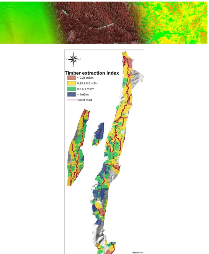
3.6.1.1 Economic availability of wood resources... 125
3.6.1.2 SFS ‐ Dissemination ... 128
3.6.1.3 SFS ‐ Digitalisation of forest communication on the basis of LiDAR data 129 3.6.2 Montafon Forstfonds ‐ New volume maps from LiDAR data ... 129
3.6.3 PAT ‐ Testing new technologies and developing methodologies... 130
3.6.4 SFI – quantifying damage following ice break event using LiDAR data ... 132
1
ABSTRACT
In the framework of the NEWFOR project several tools have been developed according to each WP goals and activities. Application of new technologies and tests of the instrument implemented in the project have been conducted in different areas among the Alpine Space. In this deliverable the most significant activities are reported. Some of them are included also in the integrating manual “Logistic Planning Strategies – Good practices for the Alpine Space”, whose text is part of this document.In this deliverablewe are presenting the activities conducted to the forest resources delineation and assessment, forest accessibility analysis, forest connectivity, cost and benefits evaluation, and the final concatenation of results. Further example of NEWFOR activities not included in the final handbook are presented in the last section of this document.
2
A SYNTHETIC OVERVIEW OF THE INTERREG ALPINE SPACE
PROJECT NEWFOR
2.1
THE CONTEXT
Although forests represent a key resource of mountain environments, their valorization is hampered by accessibility constraints that prevent an efficient mapping, management, harvesting and transport of wood products.
Forests fulfil multiple functions in mountainous areas. They have an ecological function as host of many habitats and species. They also are a leisure area for social activities such as hiking, skiing… From the economical perspective, the production of renewable resources like timber and fuelwood has positive effects both at global scale, with climate change mitigation, and local scale with rural employment and the development of a regional value chain. The objective of preserving and improving the development of mountain forests is a point of public interest. However, managing forests in mountain territories is a difficult task as topography and climate set strong constraints inside a complex socio‐economical framework.
In particular, a precise mapping of forest biomass characteristics and mobilization conditions (harvesting and accessibility) is a prerequisite for the implementation of an efficient supply chain for the wood industry. The available information is currently insufficient to provide, at reasonable costs, the required guarantees on the wood supply and on its sustainability. With the recent development of new remote sensing technologies and modelling tools, major improvements regarding the evaluation of the forest growing stock and accessibility are now possible. Upon this highly valuable information, decision‐making tools must be build to optimize the investments in forest infrastructures required for a cost‐effective wood supply while securing the sustainable management of forests, and to support the implementation of an efficient European policy for mountain forest management..
2.2
OBJECTIVES OF THE PROJECT
According to this context and based on the use of new technologies (LiDAR: light detection and ranging, Unmanned Aerial Vehicle,...) for forest and topography characterization, the project NEWFOR is dedicated to enhance and develop tools and adapted policies for decision making in the field of a sustainable and adaptive mountain forest resources management facing the sustainability of mountain forest ecosystems services.
So, the main objective of the NEWFOR project is the improvement of mountain forest accessibility for a better economical efficiency of wood harvesting and transport in a context of sustainable forest management and wood industry in changing climate.
Forest resources and LiDAR
Recent developments in LiDAR technology, combined to other available data sources (aerial photographs, aerial photo series by UAVs, …), are now allowing a precise and fine mountain forest resource quantification, qualification and mapping. Integrating this technology will provide an innovative response to the challenges of a precise and robust knowledge on the available growing stocks. The project aims at testing and developing tools that will help forestry end‐users to benefit from this technological advance.
Forest accessibility
After the identification of forest resources, the second step of an efficient forest management is to evaluate the accessibility to these resources. In mountain areas, topography is the main constraint to a technical and economically efficient exploitation. The project demonstrated how to use topographic LiDAR data coupled with geographic information systems (GIS) for an optimal planning of forest harvesting and logging while taking current and scheduled accessibility of forest resources into account.
Forest and industry connectivity
Once the forest resources and accessibility are characterized, then remains the issue of the connectivity between wood piles in the forests and wood yard of mills. This link is often neglected but is crucial for a comprehensive assessment of the wood supply efficiency. Costs and benefits evaluation
NEWFOR aims at developing decision‐making tools dedicated to the definition of strategies for sustainable mountain wood supply chain. To fulfil this objective, tools for identifying forest resources, their accessibility and connectivity to the wood market are first considered separately. In order to achieve the demarche, and to choose the optimal strategy, it is necessary to evaluate the whole workflow from the economical aspect by comparing the costs and benefits of each possible strategy.
Logistical planning strategy
There is a need to frequently adjust the planning of forest management to new economical evidence as well as to unforeseeable developments. Such an adaptive management needs to balance ecological, social and economic factors. The final objective was to provide forest managers and decision makers with reliable information for the evaluation of technical and economical conditions for their decision‐making on timber supply chain logistical planning and land use strategies.
3
GOOD PRACTICES EXAMPLE IN THE TEST‐SITES
In the framework of the NEWFOR project several tools have been developed according to each WP goals and activities. Application of new technologies and tests of the instrument implemented in the project have been conducted in different areas among the Alpine Space. In this deliverable the most significant activities are reported. Some of them will be included in the integrating manual “Logistic Planning Strategies – Good practices for the Alpine Space”, whose text is part of this document. Following the scheme of the project presented in the previous section (2.2), the activity devoted to forest resources delineation and assessment will be presented firstly (3.1), followed by forest accessibility analysis (3.2), forest connectivity (3.3), cost and benefits evaluation (3.4), and the final concatenation of results (3.5). Further example of NEWFOR activities are presented in the last section.
3.1
FOREST RESOURCES AND LIDAR
The role which mountain forests play is extremely varied. Their contribution to the stability and overall development of life and economic factors in mountainous regions is highly significant. The production of renewable resources like timber has positive effects on climate change consequences attenuation, employment and makes for a strong regional value chain, which in turn has an enormous impact on rural development. The objective of preserving and improving the efficiency of mountain forests is a point of public interest and can only be guaranteed if the planning and implementation of all respective measures are integrated into an adequate and well‐known socio‐economic context. Managing forests in mountain territories is significantly more cost intensive than in plain ones. This is due to the topographic conditions, climatic adversity and limited access which drive partly the economic context. A good knowledge of the forest biomass location, its characteristics and mobilization conditions (exploitability, service roads, and mobilization costs) is a prerequisite for an effective wood harvesting and transport and for a sustainable wood industry. This knowledge is currently insufficient to provide at reasonable costs, the required guarantees on the wood supply and on its sustainability. Improving an efficient and robust evaluation of the forest growing stocks (volume and quality) and its accessibility are the efficient measures to mobilise sustainably more wood from mountain forests. As building forest roads and other infrastructures are often complex and expensive, the availability of financial resources is a key challenge. This could be achieved by providing technology and financial support. With such knowledge and tools it will be then possible to develop an active and sustainable cultivation of mountain forests and an efficient European mountain forest management policy.
Recent developments in LiDAR technology – also called airborne laser scanning (ALS) data, combined to other available data sources (aerial photographs, aerial photo series by UAVs,…),
precise and robust knowledge on the available growing stocks. The actions of the WP4 (named “Forest Resources & LiDAR”) have the overall objective to test (i.e. benchmark for single tree detection algorithms), to optimize (i.e. for forest area delineation, growing stock assessment) and to develop new tools (i.e. growing stock change assessment, forest structure estimation) using data which are acquired by these new technologies.
Based on these overall project goals, in the framework of the WP4, the following relevant objectives were formulated:
Collection and sharing of knowledge regarding the use of an innovative remote sensing technologies
(LiDAR & UAV) for forest area and growing stocks location, forest structure assessment and single tree
parameter estimation;
Identification and testing of currently available LiDAR data processes and development of new processes
adapted to mountain conditions in order to obtain the actual distribution of growing stock, stand structure
and other parameters useful to characterize mountain forests;
Determination of the LiDAR data to be acquired on pilot areas to obtain a detailed map of the volume
distribution and forest structure;
The results of WP4 are the basis and prerequisite for WP5 to 8 (see following chapters), building the background for the setting up of specific models dedicated to an adapted logistic planning strategy taking into account the accessibly and availability of growing stocks, the economic conditions and the mountain forest ecosystems services.
3.1.1
FOREST AREA DELINEATION
A fundamental task in forest management is locating and analysing forested areas. The delineation of forested areas has a long tradition in forestry and therefore worldwide different forest definitions exist to define whether an area can be classified as forest or non‐forest. The delineation task is critical as a broad field of applications (i.e. obligatory reporting) and users (i.e. governmental authorities, forest community) rely on this information. The results determined from these applications are highly dependent on the fundamental input parameters size and position of the delineated forest areas. In the past mainly aerial images were used for a manual or semi‐automated delineation. Shadow effects limit this task, particularly for detecting small forest clearings and the exact delineation of forest borders on a parcel level. Additionally, the quality of the results of a manual delineation is subjective and variable between interpreters and may lead to inhomogeneous, maybe even incorrect datasets. An automatic delineation of forested areas based on LiDAR data can overcome these limitations in most cases. Within the NEWFOR project the method of Eysn etal. (2012) was applied to several NEWFOR pilot areas characterized with different forest structure and growing conditions to detect forested areas. The method relies on four clearly defined geometrical criterions (min. area, min. height, min. width and min. crown coverage) which are subsequently checked against LiDAR data. The criterion land use is not considered as this information can hardly be obtained from remote sensing data. Other data sources, such as the cadastre, are needed to gather this information.
From a hierarchical point of view, the four geometrical criteria have equal rights. To apply these criteria to remote sensed data, a hierarchy has to be defined with respect to a processing chain. For instance, it would make no sense to check the minimum forested area if there is no potential area detected yet. In this approach, the hierarchy is defined as follows: (1) min. height, (2) min. crown coverage, (3) min. area and (4) min. width, whereas (3) and (4) are checked in an iterative process. The minimum height criterion is applied by height thresholding the canopy height model within the vegetation mask. For the crown coverage calculation the ‘tree triples’ approach as described in Eysn etal. (2012) was used. This approach provides a clearly defined reference size for calculating the crown coverage and overcomes limitations such as smoothing effects or dependency of the kernel size and shape of the moving window approach, especially in loosely stocked forests. The crown coverage value is calculated for each tree triple independently and therefore an interaction with neighbouring triples is not considered. The minimum area criterion is applied by using standard GIS‐queries. The areas of all valid polygons are calculated for the potential forest mask fulfilling the height‐ and crown coverage‐criterion. The minimum width criterion is applied by using morphologic operations (open, close) based on the intermediate result fulfilling the criteria height, crown coverage and area. For this operation, a circular kernel with a radius of 5 pixels (pixel size 1 × 1 m) is used to eliminate narrow forested areas that do not fulfil the criterion. This operation is also related to the area criterion, because the removal of narrow areas leads to changes of the forested areas. Therefore, an iterative process of checking minimum area and width is applied.
The usage of these clearly defined geometrical criterions as defined in the method of Eysn etal. (2012) delivers robust, repeatable and comprehensible delineation results. This is significant when the results are used for obligatory reporting or change detection based on multi‐temporal data. Especially at loose stocked forests where the forest / non‐forest decision is demanding the most the proposed technique for checking crown coverage works reliable (Figure 1). The method is fully automatically, can be applied to large areas and fulfils the requirements of an operational application. Different forest definitions can be considered by the method. Therefore an application to different areas / countries with different restrictions is enabled. Furthermore the method was easily applied to the local forest definition requirements of the different pilot areas within the NEWFOR project. For the pilot area Immenstadt in Germany the automatically derived forest mask was compared to a manually delineated reference mask. The resulting confusion matrix shows a Kappa of 0.83 and an overall accuracy of 93%.
Figure1: Delineationof forestedareasbasedonLiDARdata.A)orthophoto ofaloosely stocked forestB)EstimatedtreecrownsanddetectedtreetriplesbasedonLiDARdataC)Delineatedforest areas(presentedsemi‐transparentasoverlayofaz‐codedcanopyheightmodel
3.1.2
FOREST STRUCTURE ASSESSMENT
In the following sections, four approaches for the derivation of structurally relevant parameters from ALS data are described. These are (1) crown segments (2) compactness of vegetation (3) vertical layer structure (VLS) of vegetation and (4) canopy cover (CC). These parameters exploit the information collected by ALS to describe vegetation structure and how different patches of vegetation are inter‐connected in terms of vertical structure of the plants building the patches. The main aim of the crown segmentation is to extract individual trees in forested areas. In the approaches described here, the segments are also used as reference unit for the calculation of structural parameters based on the 3D point cloud. To create the tree crown segments, an edge‐ based segmentation procedure is applied on the nDSM (Höfle etal., 2008). It delineates convex shapes in the nDSM by finding concave edges between them. The main criterion for the edge detection is a minimal curvature in the direction perpendicular to the direction of the maximum curvature.
The compactness of vegetation refers to the relation of a vegetation patch’s surface, defined as the area of its enveloping canopy, to the volume enclosed by it. Thus in the following text it will be referred to as surface‐to‐volume ratio. The parameter basically relates to the 3D shape of a vegetation patch and how the patch is inter‐connected with other patches. It is calculated on the basis of a so‐called difference DSM (DSMdiff), which comprises the height difference of the highest and lowest occurring ALS echo in a grid cell without consideration of terrain echoes. The
DSMdiff is a measure of vertical vegetation extent, its multiplication by the grid width results in the vegetation volume. The vegetation surface is derived as the sum of the area of all visible lateral faces, the top and the bottom face of a cell column in the DSMdiff. Finally, the ratio of the surface and the volume are computed for each raster cell and assigned to the vegetation segments (Mücke etal., 2010).
For the derivation of the VLS and the CC the capability of ALS to penetrate the foliage and to provide direct height measurement of canopy and sub‐canopy strata, as well as the forest ground is exploited. A so‐called penetration index for different vegetation height intervals is calculated based on the 3D point cloud as a measure of penetrability and geometric structure. The definition of the height intervals can either be done in an absolute (i.e. a‐priori fixed heights for each level) or in a relative way (i.e. percentage of maximum occurring height). To enable a comparison of the layer structure information assessed by the forest inventory (FI) and the ALS data, the ALS data within the FI sample plots were extracted. At the GPS measured positions of the sample plot centres the ALS data were selected within the area of a sample plot plus a buffer zone of e.g. 1 m to consider border effects. The DTM was used to calculate the normalized echo heights of the single ALS echoes, which were subsequently needed for the selection of the echoes belonging to the respective height levels as defined in the FI. For every defined height level, a 1 m resolution raster map was created containing the number of ALS echoes in each cell. If a cell contained ALS echoes, it was counted as covered. The sum of all overgrown cells per height level results in the total CC of a single height level.
Additionally, an area‐wide forest structure map was derived on the basis of e.g. relative height intervals (i.e. 0‐33%, 34‐66% and 67‐100% of the maximum relative height per each before derived crown segment). For each segment the number of points per height layer and the total number of vegetation points are determined. Finally, the ratio of these quantities (penetration index) is computed (Mücke et al., 2010). For the generation of the forest structure map a decision tree based classification approach is used to classify the segments and determine the number of vertical forest layers based on the penetration index.
Generally it can be stated that the delineation of single trees or tree crowns in dense deciduous forests is a challenging task. As the applied segmentation algorithm detects convex objects separated by concave areas, it works very well for single trees with clearly distinct crowns. But especially older or larger deciduous trees often develop large crowns with multiple maxima which results in multiple convex areas and these are therefore represented by more than one segment. A further limitation occurs in very dense young deciduous forest, characterised by a smooth canopy surface leading often to segments that include multiple trees.
The vegetation surface‐to‐volume ratio can be seen as a proxy for the compactness of a particular landscape element. Changing compactness along a geometric element implies a change in structure and consequently permeability. This permeability is of significance for certain species, e.g. highly adapted birds, whose requirements do not allow structural changes
It is clearly visible in the ratio image that the character of the vegetation structure is changing significantly below the power line. For evaluation of the results, visual examination of the 3D point cloud had to be used, because of the lack of an adequate ground truth measurement method for the proposed surface to volume ratio. A profile view is given in Figure 2b. It can be seen that the changing of the corridor vegetation character, as indicated by the ratio, is supported by the 3D point cloud. In this case the power line acts as a natural barrier, which is a disturbance in this particular habitat or corridor.
Figure2:(a)surface‐to‐volumeratiocalculatedonsegmentbasis,(b)verticalprofileofthepoint cloudshowingthedifferingcharacterofvegetationinanareawherealsothesurface‐to‐volume
ratiosignificantlychanges(adaptedfromMückeetal.,2010).Terrainpointsareinyellow, vegetationpointsareinturquoise.
In Figure 3 the canopy cover maps of individual a‐priori fixed height levels (V1, V2 and V3) are shown. The total CC is shown in V4. For quantitative evaluation of the results of the derived layer structure and CC on plot level, scatterplots were derived (see Figure 4). All three single levels V1 to V3, as well as the total CC represented by level V4 exhibit significant scattering. The upper levels V3 and V4 reveal a linear relationship of FI‐ and ALS‐derived CC. However, linear relation is only weakly distinguished in the lower levels V1 and V2, clearly showing an underestimation by the ALS‐based method because of the absence of echoes in this canopy strata. This indicates that future research on this topic will need to concentrate on the development of a predictive model describing the relationship of FI‐ and ALS‐based layer structure and CC, and considering the drawback of missing echoes in any stratum.
Figure3:ExampleofcanopycoverderivationbasedonALSechodistribution.LevelsV1(brown) andV2(green)clearlyshowanunder‐representationoftherespectiveverticallayersduetothe
lackofechoes.
Figure4:ComparisonofFI‐ andALS‐estimatedcanopycover.
Figure 5 shows a resulting forest structure map and two profiles of the 3D point cloud, which are meant to display the structural diversity. Four dominant types of vegetation structure could be identified: L1 + L3 > 80% (red), L2 + L3 > 80% (light green), L3 > 80% (dark green) and equally distributed structure (yellow). Below the profiles the corresponding lines from the forest structure map are given. They demonstrate that the classification result corresponds very well with the actual structure of the forest. Deviations could be observed in areas with high local variations, which cannot be accounted for by using the proposed method because inner segment variations are not considered.
Figure5:Left:Foreststructuremapcalculatedonsegmentbasis(whitelinesshowprofile locations,whiterectangleNr.3showslocationofFigure2).Right:ProfileviewsoftheALSpoint cloud.Belowtheprofilesthecorrespondinglinesfromforeststructuremaparegiven(adapted
fromMückeetal.,2010).
3.1.3
GROWING STOCK ESTIMATION
A common way to acquire information about forest resources is to perform terrestrial forest inventories. The obtained information is spatially limited and therefore area wide forest management in terms of harvesting planning is limited. Remote sensing technology i.e. LiDAR allows an area wide mapping of the forest resource (i.e. growing stock) and provides the forest community with information suitable for area wide planning. Integrating this technology into the wood supply chain can provide an innovative response to the challenges of a precise and robust knowledge on the available growing stocks. A limitation of many LiDAR based growing stock models is the lacking sensitivity to local forest conditions. This means that growing stock models are often calibrated for large areas, local changes of the forest structure are not considered and the resulting models are smoothing the local situation. Within the project NEWFOR the model of Hollaus etal. (2009) was applied to several pilot areas located in different Alpine Space countries in two different ways: A) A general growing stock model was calibrated and applied for entire pilot areas and B) growing stock models were calibrated for different strata. For the stratification different information obtained from remote sensing data was used. This information can for example be a tree species classification as presented in Waser (2012) or a crown coverage map as presented in Eysn etal. (2011). The calibrated models were applied and tested for the NEWFOR pilot areas.
For estimating the growing stock the method described in Hollaus etal. (2009) is applied. This method assumes a linear relationship (Eq. 1) between the growing stock and the ALS derived canopy volume, stratified according to four canopy height classes to account for height dependent differences in canopy structure.
m i i i FIv
v
1 , can 410
(Eq.1)where vFI represents the stem volume (m³/ha), calculated from the forest inventory data, m is the number of canopy volumes and is set to four and i are the unknown model coefficients. The canopy volumes (vcan,i) are calculated based on Eq. 2.
i i
i
p
ch
v
can,
fe,
mean, (Eq.2)where pfe,i represents the relative proportion of nDSM pixels within the corresponding canopy height class to the total number of nDSM pixels within a circular sample plot area with a radius of 12 m and chmean,i is the mean height of the nDSM pixels within the corresponding canopy height class. The four canopy height classes are defined with the following height limits:
ch1 ‐ 5 m to 15 m, ch2 ‐ 15 m to 25 m, ch3 25 m to 35 m, ch4 ‐ 35 to 50 m.
The stratification based on remote sensing data was carried out fully automatically and is applicable to large areas. The criterion “species” classified the forest into areas of deciduous, mixed and coniferous forest, whereas the primary species classification can be derived from classification of aerial images as for example described in Waser (2012) or from full‐waveform ALS data classification as shown in Figure 8. The criterion “crown cover” classified the forest into areas with dense or sparse coverage. In total six different models can be calibrated and applied using these criterions. In contrast to a general model without stratification the stratified model increased the accuracy. This was expected as the general model does not account for local changes in the forests appearance and different strata might be incorrectly represented (Figure 6).
Rightimage:Subplotofthetwoclassesconiferousdenseandconiferousloosestocked.Theclass coniferousloosestockedisclearlyunderestimatedinthenonstratifiedmodel.
The relative standard deviation of the residuals between estimates and reference could be enhanced by 4%. The results of the tests within the project prove that growing stock maps with very high spatial resolution can be derived from remotely sensed data. These maps allow comprehensive forest management for large areas and serve as input data for various forest planning activities. The level of detail of growing stock maps in operational use is still under discussion. However, this discussion within the project consortium show a first trend for aggregating the resulting growing stock map, because it is too detailed for most applications. The aggregation could be performed by resampling the data to cell sizes of several meters (see Figure 7) or by aggregating the data to stand levels or to forest management units.
Figure7:DerivedgrowingstockmapforasubsetofthepilotareaMontafon,(left)1.0mand(right) 5.0mspatialresolution.
In Figure 8b the classification result into coniferous and deciduous forest based on full‐ waveform ALS data is shown. The classification can be used for stratified growing stock modelling as shown in Figure 8c.
Figure 8: (a) Orthophoto ©Bing maps, (b) classified tree species map and (c) tree species dependentstemvolumemap.
3.1.4
GROWING STOCK CHANGE DETECTION
The high potential of airborne laser scanning (ALS) data for forestry applications has been confirmed in many studies during the last decade. The open question is still the application of ALS data for monitoring applications. Due to the ALS data acquisitions costs re‐acquisition are rare until now. Consequently there is on one hand a lack of data and on the other hand a lack of knowledge of using multi‐temporal ALS data for forest monitoring tasks.
Therefore, the capabilities of ALS data for operational forest monitoring of growing stock were analysed in the pilot area Montafon, Austria. In addition to two ALS data sets forest inventory data for both ALS acquisition times are available for this study.
In the first processing step topographic models are calculated and differences between the models originating from inaccuracies in the georeferencing are minimized. To avoid errors in the assessed growing stock change originating from digital terrain model (DTM) errors due to different terrain point densities, one reference DTM is used for both dates. It is assumed that the DTM within the forests do not change during the two ALS acquisitions. Thus the DTM is determined from the ALS data set with the higher point density to derive a DTM with higher accuracy. For the calculation of the DTM the hierarchic robust filtering approach described in Kraus and Pfeifer (1998) is applied, which is implemented into the software Scop++ (2012). For the derivation of the digital surface model (DSM) a land cover dependent approach described in Hollaus et al. (2010) is applied. This approach uses the strengths of different algorithms for generating the final DSM by using surface roughness information to combine two
through the k‐nearest neighbours). Finally the two nDSMs (DSM2004, DSM2011.) are calculated by subtracting the DTM from the DSMs. The spatial resolution of all topographic models is 1x1 m². The differences of the DSMs have shown that especially height differences of stable objects between the two surface models originating from strip differences or errors in the georeferencing have to be minimized using e.g. a least square matching (LSM) in a first step. The calculated normalized digital surface models (nDSMs) are used as input for the growing stock regression models (see previous chapter). Each data set is calibrated with the corresponding FI data and the derived growing stock maps are compared.
For differentiating between exploitation and forest growth the area is classified into areas with an (a) increased (= forest growth) and (b) decreased (= exploitation) surface height. As for each ALS data set small differences in the tree crown representation within the DSMs can occur morphologic operations (i.e. open / close) and a minimum mapping area of 10 m² are applied to the DSM difference map. For each classified area (exploitation, forest growth) the changes for the assessed growing stock is analysed separately. To test the transferability of the calibrated growing stock models from acquisition time to the other, the calibrated models are applied to the ALS data which was not used for the calibration. Finally the derived growing stock maps are validated with the corresponding FI data.
In Figure 9a an orthophoto overlaid with the mask of corresponding objects that are used for the LSM is shown. These objects represent mainly open areas, roofs and streets and are distributed over the entire area. In Figure 9b the DSM difference map (DSM2011‐DSM2004) is shown and indicates a vertical shift between the DSMs of 0.17 m averaged for the masked objects. Calculating the LSM of the identified objects 3D shift parameters are determined and applied to the DSM2004. In Figure 9c the difference map between the DSM2011 and the shifted DSM2004,LSM is shown, whereas the average difference is minimized to 0.07 m. Due to this height adjustment the remaining height differences can mainly be connected to changes of tree heights and consequently to growing stock.
Figure9:(a)Orthophotosfrom2012withaspatialresolutionof0.25moverlaidwiththemaskof correspondingobjectsthatareusedforLSM,(b)differenceofDSMs(DSM2011‐DSM2004)beforeand
(c) after the LSM.Red colours indicateexploitation of forest,green/blue colours indicateforest growing.
It could also be shown that the growing stock changes derived from the estimated growing stock maps are similar to those derived from the forest inventory data. For both models a similar accuracy could be achieved. The relative standard deviation derived from cross validation is rather high for both models and can mainly be explained by the angle gauge measurement using only one fixed basal area factor of four, which leads to discontinuities in the statistically calculated FI growing stocks on a plot level. A further explanation is the fact that for the first ALS data set the ALS flights took place between 2002 and 2005, whereas the FI data was collected in 2002. This means that changes in the DSM (i.e. forest growth, exploitation), which are available
To test the transferability of calibrated models to other ALS acquisition times the calibrated model from 2011 was applied to the ALS data from 2002‐2005. The corresponding scatterplot shows a very high agreement between the two models. A similar result is derived for the ALS 2011 data.
In Figure 9 the difference map of the estimated growing stocks (2011‐2004) overlaid with the detected exploitation areas is shown. The visual validation shows that the applied work flow for detecting harvested areas work well even on the level of single trees. Using GIS tools the total amount of harvested growing stock can be calculated for example for each exploitation polygon. For the estimation of the forest growth an averaging within homogenous areas (e.g. forest stands) is required to avoid errors originating from different tree crown representations (i.e. due to varying ALS point density, ALS sensors, ALS acquisition properties, wind effects, etc.) on a single tree level. Based on the FI data the growing stock increased from 2002 to 2011 of 43.0 m³/ha in average for the used 184 sample plots. Using the estimated growing stocks derived from the ALS data an average difference of 42.5 m³/ha is observed.
Based on the findings of this study it can be stated that ALS data is an excellent data source for change detection of forest parameters (i.e. growing stock). Furthermore these analyses have shown for the first time that calibrated regression models can be transferred to ALS data from different acquisition times, which opens up interesting possibilities for operational forest inventories.
Figure 10: Differencemap of estimatedgrowing stocks(2011‐2004)overlaid with the detected outlinesoftheharvestedforestareas.InthebackgroundaCIRorthophotoisshown.
3.1.5
SINGLE TREE DETECTION / BENCHMARK
A single tree detection benchmark based on airborne laser scanning data was carried out to show the potential of existing single tree detection methods. A unique dataset originating from different regions of the Alpine Space, covering different study areas, forest types and structures, was used within this benchmark. In total eighteen study areas in five countries in the alpine space were investigated (Figure 11).
Figure11:Studyareasusedforthesingletreedetectionbenchmark
For all study areas ALS data and a digital terrain model (DTM) were provided to the benchmark participants. Based on these data the participants had to automatically extract single tree information by applying their algorithm. In total seven Institutions applied their Methods to the Benchmark dataset (Table 1). The minimum requirements were the extraction of tree position and tree height as well as a description of the used algorithm / workflow. Forest inventory (FI) measurements (fully calipered plots) were used as a reference to test the different detection results.
The benchmarking process covers seven general steps. Initially a quality check of the input data (1) was performed. This was followed by the detection process of the partners using their methods (2), the matching process to link the detection results to the ground truth data (3) and finally the investigation of the matching results. The benchmarking results are prepared in different Levels of Information (LoI), starting with investigations based on study area (LoI‐4) and detection method (LoI‐3). Additionally investigations per forest type (LoI‐2) and an overall performance (LoI‐1) of the benchmark are presented.
The quality check of the ALS and FI data was carried out to ensure a consistent level of quality. All study areas are sufficiently covered by ALS data. The ALS data are free of gross errors. Heterogeneous point densities from 4 points / m² up to 120 points / m² are given. The quality of the FI data was investigated by performing a questionnaire regarding the FI data. The responsible NEWFOR partners reported information regarding absolute and relative accuracy of the FI data as well as general information about the study areas.
For absolute Georeferencing GPS is widely used for surveying the plot location. In a post‐ processing step the plots were manually co‐registered to the Remote Sensing data. The estimated absolute accuracy after manual co‐registration is ± 2.0 m.
State of the art for relative tree measurements within a plot is using compass bearing and tape / electronic ranging for measuring tree positions and using a Vertex system for measuring the tree heights. The reported relative accuracy varies from ± 0.3 m to ± 1.0 m for the horizontal part. For the vertical accuracy a value of ± 1.0 m was reported by all partners.
2) Single tree detection by participants
In total eight methods were applied to the Benchmark dataset (Table 1). Most methods rely on local maxima detection in a rasterized CHM. Beside that also purely point cloud driven methods were applied. All participants were able to apply their method to the given dataset.
Table1:OverviewofAppliedMethods
ID PP Name Method Type
1 LP Irstea LM+Filtering R
2 PP5 FEM LM+Region Growing R
3 PP7 SFI LM+Multi CHM R
4 PP10 TESAF LM+Watershed R
5 PP11 SLU / TU Wien Segmentation+Clustering R+P
6 PP11 TU Wien 3x3 LM3x3 R
7 PP11 TU Wien 5x5 LM5x5 R
8 PP12 SFS Polyn. Fitting+Watershed R
R…Raster; P...Point Cloud; LM…Moving Window for local Maxima 3) Matching process
A fully automated matching procedure for linking the detection results (test trees) to the FI data (reference trees) was established and applied for the NEWFOR single tree detection benchmark. This methodology enables clear and reproducible testing.
In this paragraph a short summary of the matching procedure is given. Starting from the highest test tree within a study area, the restricted nearest neighbouring reference trees within a defined neighbourhood are detected and marked as matching candidates. Restricted nearest neighbouring introduces height criterions and neighbourhood criterions which need to be fulfilled to match two trees (Figure 12). Trees with the best neighbourhood and height scores are matched. This means that not always the “simple” nearest neighbouring trees are connected. The procedure is applied to all detection results of the participants. The outputs of the matching process are qualitative and quantitative statistical parameters as well as vector layers for being displayed in a GIS system.
A visual inspection of the matching results shows a good agreement (Figure 13). The height and neighborhood criterions ensured correct matching results in most cases. Especially the height criterion ensured that tall trees are not connected to nearby small trees. The results of the automatically matching were validated by visually interpreting 699 randomly selected matching results in a GIS environment. The manual interpretation shows an Overall Accuracy of 97%.
Figure 13: Automatic matching result of participant “LP‐Irstea” for study area 16. The data is displayedasoverlayofacanopyheightmodel(CHM).
The following quantitative statistical parameters about detection rates and spatial accuracy are presented:
‐ Matching (assignment) rate Total number or rate of matched trees
‐ Commission rate Total Number or rate of Test trees which could not be matched ‐ Omission rate Total number or rate of Reference trees which could not be matched ‐ HMean Mean of horizontal matching vectors (2D Vector between Test and Reference) ‐ VMean Mean of tree height differences (ΔH between matched Test and Reference) Additionally summarizing statistics (Root mean square) are presented if multiple study areas or methods are investigated.
The results of the matching process are presented in different LoI. LoI‐4 enables exploring the detection results on the study area level while LoI‐3 gives information on the method level. LoI‐2 shows the results for different forest types. Finally, LoI‐1 shows the overall performance of the benchmark.
For all LoI the qualitative and quantitative parameters obtained in the matching process were plotted in two different Barplots. One plot focusses on the different rates found in the matching process while the other focusses on the spatial accuracy. The Barplot “Matching Rates” is sorted upwards to the Commission rates. An Example is presented in Figure 14. For LoI‐4 the amount of trees in different height classes were plotted in additional Barplots.
Figure14:Barplotexamplesforthedetectionratestatisticsandthespatialaccuracystatistics.
Detection results on the study area level (LoI‐4)
In general, it could be seen that the vertical distribution of tree heights seems to have a major impact on the detection / matching results of the different methods. The more the trees are vertically distributed the lower the matching rates are. The matching rates in different height layers indicate that especially in the lower height layers more advanced methods as for example 3D clustering in the point cloud can detect more trees than methods that rely on local maximum detection based on a rasterized canopy height model
Matching results with a high matching rate combined with a low commission rate indicate a good matching result. The best detection result was obtained for an old forest stand with high trees and no understory vegetation. The lowest detection result was obtained for a multi layered forest with a high amount of trees in different height layers. In a summarized view the results show that multi layered forests are challenging for all tested methods.
It can be assumed that a higher point density can be linked to a higher penetration rate and therefore small trees in subdominant layers might get mapped more efficiently. One tested study area shows a point density of 121 pts / m² and the inventory data shows a strong vertical distribution of the given trees. Even with this very high point density only the worst detection result of all study areas could be obtained. It seems that even very high point densities do not help to achieve better detection results for complex forest structures. However, investigating the effect of different point density on the detection results was not scope of this study.
Detection results on the method level (LoI‐3)
variable window sizes in the moving window approach. The variability of the kernel size seems to be an advantage compared to methods based on static kernel sizes.
The method of PP5‐FEM shows comparable matching rates to the method of LP‐Irstea but shows a twice as high commission rate. In the lower height layers up to 10 m tree height only up to 5% of the extracted trees could be correctly matched. However, the method is based on rasterized ALS data and therefore the rather low matching rate in the lower height layers was expected. The methods PP7‐SFI and PP11‐SLU are based on 3D operations in multiple canopy height models or directly in the 3D point cloud while method PP11‐TU3x3 is based on local maximum detection in a canopy height model which uses, compared to others, a small kernel (3x3 pixels). High Commission rates in the results of these methods indicate over performance which means the methods produce high commission rates. Beside the fact of high commission rates the method of PP11‐SLU shows up to 17% of correctly matched trees in the lower layers up to 10 m tree height. Compared to other methods this is clearly the best result.
The method of PP10‐TeSAF shows a good matching rate but unfortunately also the Commission rate is high, which means that the method found many trees which could not be linked to the reference data. In the lower layers below 10 m tree height up to 7% (RMS) of the available reference trees were correctly matched.
The method of PP12‐SFS shows a high matching rate paired with a low Commission rate. Based on these values the results of PP12‐SFS are close to the results of LP‐Irstea and are one of the best within this benchmark. In the lower levels with tree heights up to 10 m the method obtained a matching rate of up to 9 % which counts together with PP20‐TESAF and PP11‐SLU to the best obtained result. Like other methods that rely on maximum search in a rasterized CHM the low rate can be explained by the methodology.
Detection results based on forest type (LoI‐2)
The class of single layered coniferous forests shows the best results of all tested classes. This result seems feasible as coniferous trees show, in most cases, a clearly defined tree crown shape. This means that the tree top appears as a clear peak in the canopy height model. Since most of the tested methods within this benchmark rely on local maximum detection a canopy height model, the good result for single layered coniferous forests was expected. The best performing methods for this forest type were the methods of LP‐Irstea, PP10‐TESAF and PP5‐SFI.
The class of multi layered coniferous forest as well as the class of multi layered mixed forest show the lowest matching rates in this benchmark. The commission rate of the multi layered mixed forest is twice as high as the rate found for the multi layered coniferous. The low matching rate can be explained by the methodology of the tested methods. Trees in lower layers are challenging for all tested methods. The high commission rate for the multi layered mixed forest can be linked to more complex crowns for deciduous trees. The best results for the multi layered coniferous forest were obtained by PP12‐SFS, PP10‐TESAF and PP5‐FEM. The best
results for the multi layered deciduous forest were obtained by PP12‐SFS, PP10‐TESAF and LP‐ Irstea.
The single layered mixed forest shows the second best matching rate for the classified results. Unfortunately a very high commission rate is given. The high rate can be explained by the fact that deciduous tree crowns tend to be more complex than coniferous ones. Single tree crowns may consist of multiple local peaks in the canopy height model that may be correctly detected as local maximum but do not represent the tree stem. The best performing methods for this forest type are LP‐Irstea and PP12‐SFS.
Overall performance (LoI‐1)
The overall performance brings together all matching results from all tested methods. An overall matching rate of 47 % (RMS) was found (Figure 15). This value aligns with the Benchmark results of other published single tree detection benchmarks. The overall best performing methods are LP‐Irstea, PP12‐SFS, PP5‐FEM and PP11‐TU5x5. The other four methods show too high commission errors. For the spatial accuracy, a horizontal accuracy of 1.7 m (RMS) and a vertical accuracy of 1.0 m (RMS) could be obtained. These values are comparable to other previously carried out benchmarks. The performance of the different methods differs more for the tree detection than for the extracted tree heights.
Figure15:OverallperformancewithintheNEWFORsingletreedetectionbenchmark.
It could be shown that forest inventory data can be automatically linked to remotely sensed data. The summary of the single tree detection benchmark provide a good overview of the performance of the different detection algorithms for the individual forest properties and can therefore support practitioners for selecting the appropriate algorithm for detecting single trees.
3.1.6
DERIVING MULTI‐SCALE FOREST INFORMATION MAPS BASED ON
ALS RASTER DATA
The communal administration StandMontafon Forstfondsmanages a forested area of almost 89 km² in the Montafon valley (Austria, Vorarlberg). Forests cover a large extent in predominantly steep terrain at 1200 m above sea level and higher. These forests provide vital protection against avalanches, rock fall, debris flows and landslides to the villages and infrastructural facilities. Spruce forests (Piceetum) predominate, mixed forests composed of
Piceaabies, Abiesalba, and Fagussylvatica (Abieti‐Fagetum) as well as beech forests (Fagetum)
can be found at lower altitudes. ALS data is available for the complete area from two time steps (2002/2004 and 2011, point density between 4‐60 pts/m²). Data from the first acquisition were already examined in terms of their useful integration in forest management planning. Based on these first experiences (cf. Maier et al, 2008) the demand for multi‐scale information maps derived from ALS data has been formulated (deductive approach):
The information maps should reflect height information of forest canopy within a 3‐level image object
hierarchy. The hierarchy represents a lower (similar to) tree crown level (TCL) and a higher forest
stand level (FSL), which are derived by segmentations of the normalized digital surface model (nDSM,
GSD: 0.5 m) and/or derivatives. An additional, more generalized, segmentation level above (TopoL)
should represent specific site conditions driven by topography factors. The image segments on the
highest level reflecting a combination of objects of the lower levels, criteria to define the delineation
of these larger objects are based on the digital terrain model (DTM) and derivatives;
The derived image objects should fulfil certain criteria (deductive approach) relevant for forest
management: TCL should reflect a median area of 25 m², a median area to border ratio of ~0.9
(compactness indicator). FSL should reflect a median area of 530 m², a median area to border ratio of
~3.7 ;
The method should be reproducible, transparent and repeatable for the application on future ALS
campaigns;
The target scale for the final height information maps should be 1:5000 for in‐field use and forest
management planning.
Following these requirements the implementation was conducted in an object‐based image analysis (OBIA) environment, allowing the integration of additional input data (forest mask, administrative units) and the connection of image objects, rasterized ALS data as well as ALS point cloud data.
The multi‐resolution segmentation algorithm (Baatz and Schäpe, 2000) was selected for the regionalization of the ALS raster data on the three different scales. The classification for TCL and FSL was based on the tree height classes referring to forest development stages used in regional practical context. The 90th percentile per object served as the height classification basis. In addition, the objects were attributed with several information derived from the rasterized ALS data.
For obtaining representative results according to the object‐size and object‐form requirements, an iterative segmentation and classification algorithm was developed in CNL (Cognition Network Language, applied in eCognition 9.0, Trimble Geospatial). The algorithm was tested on two subsets with an extent of 2500 x 2500 m. The iteration was fully automated, the relevant parameters changed for each iteration (scale parameter by increments of 5, whereas the shape parameter and compactness by increments of 0.1). To obtain ‘meaningful objects’ for forest managing purposes a different combination of input data on the FSL was tested. Combinations tested encompassed calculations of nDSM and nDSM filtered within a 3 x 3 median window, as well as the filtered nDSM in combination with the slope derivative of the DTM (to incorporate specific characteristic of the mountainous area). Based on the huge amount of resulting segmentation and classification layers, the algorithm automatically selected a subset, matching best with the deductive requirements. Figure 16 shows the result of the approach for a subset of the area.
The subsets of segmentation and classification results were cross‐checked by image interpretation experts, and the short‐listed results were successfully validated by practitioners and forest managers in the field. Selected parameters for building the 3‐level image object hierarchy are given in Table 2.
Level layer
scale
parameter shape compactness
TCL nDSM 10 0.6 0.6 FSL nDSM (3x3 median filtered) Slope of the DTM 50 0.6 0.4 TopoL DTM Hillshade of DTM (sun inclination = 42.5°; sun azimuth = 180°) 1000 0.5 0.5
Table 2: Selected parameters for building image object hierarchy by using multi resolution segmentation.
Figure16:Subsetofthe resultingmulti‐scaleforestinformationmaps (right:FSLlayer,left:TCL layer). Coloursare indicatingtree heightclasses referringto forestdevelopmentstages usedin regional practical context. Patches are classified according to to the 90th percentile of height above ground; no colour:<1.3 m or not forest, yellow:1.3 to 6m, light green:6 to11m, dark green:11to22m,lightblue:22to29m,darkblue:29to33m,red:>33m.
Based on the field validation the final maps were calculated for the Montafon area (ca. 237 km2 forested and ca. 89 km2are maintained by Stand Montafon), resulting in a database of almost 7 million objects on the TCL, 300,000 objects on the FSL and 8,000 objects on the TopoL. The object‐based image analysis with a multi‐level segmentation (Figure 17) followed the strategy of (1) data pre‐processing: including the steps of merging (LiDAR‐)image mosaics (105 mosaics with size 2500 x 2500 m) and calculating derivatives, (2) incorporating additional data of a forest mask layer and administrative boundaries and (3 to 5) segmenting FSL, TSL and TopoL, as well as calculating a merged FSL layer and exporting object feature statistics of each layer (object size, object perimeter, object to perimeter ratio, several percentiles of height, minimum
and maximum values of height, standard deviation of height). Finally TCL and FSL were classified according to the above mentioned classification scheme.
DATA
105 Mosaics á 2500 x 2500 m =
656.25 km2; (ca. 237 km2
forested and ca. 89 km2 are maintained byStand Montafon)
Parameter Layer = nDSM Scale parameter= 10 Shape= 0.6 Compactness= 0.6 Parameter Layer = nDSM median 3x3 + DTM slope Scale parameter= 50 Shape= 0.6 Compactness= 0.4 Data pre‐ processing L1: Tree crown level L2: Forest stand level Additional DATA
Forest mask layer
Administrative boundaries L2 merg ed : Fo re st st a n d le ve l me rg ed L3: Topography level MR S se gm en ta ti o n Forest mask Merging mosaics of nDSM and DTM Calculation: DTM Hillshade Calculation: DTM slope Calculation: nDSM median filter 3x3 MR S se gm en ta ti o n MR S se gm en ta ti o n Parameter Layer = DTM + DTM Hillshade Scale parameter= 1000 Shape= 0.5 Compactness= 0.5
1.
2.
3.
4.
5.
Figure17:Strategyonderivingmulti‐scaleforestinformationmapsoftheMontafonarea(ca.237 km2forested).
3.1.7
NEW REMOTE SENSING PLATFORMS / UAVS FOR FOREST
APPLICATIONS
UAV – unmanned aerial vehicles are a rapidly upcoming method for remote‐sensing data acquisition, mostly aerial images and derived products. By now, the systems are light‐weight and cost‐effective, the development and miniaturization of the sensors and their reliability enable a relative safe operation with good chance of success. UAV´s are quickly ready for operation almost everywhere and every time. Limitations – specially in mountainous and forested environments ‐ result mainly from weather conditions (wind!), visibility, availability / existence of landing sites, GPS signal quality and last but not least legal constraints.
Most common forms are small, electrically powered model planes with wingspans from 2–3 meters and multi‐ and helicopter respectively. They are piloted by an operator via remote control (RC), assisted by an autopilot on‐board (Figure 18).
Figure18:Fixed‐wing UAV,builtandusedinNEWFOR‐project.(www.bfw.ac.at); Fixed‐wingUAV “Mentor”(left),startingtheUAV(right).
Autopiloted UAV´s are navigated by a small on‐board GPS/INS‐unit. At the ground station, the mission planning is prepared and flight path, flying height, velocity and trigger are defined. The mission itself runs fully automated, wireless communication allows tracking the actual position of the platform and adapting the flight plan if possible. In addition the fully automated mode, a semiautomatic and a manual mode, e.g. for landing in case of signal loss or other unexpected problems, is available. The flight has to be supervised by a qualified pilot, who is able to take over the direct control of the UAV. The range of the UAV depends mostly on its size and shape, because it always has to be visible and controllable for the pilot. The maximum flying distance for the above mentioned “Mentor“ is about 1000 meters. Flight‐attitude data are logged and either transmitted to the ground station in real time or downloaded after the flight. If synchronized with the camera‐data the position and angles of the camera can be reconstructed (parameters of exterior orientation, EOP).
Technical limitations can hinder the acquisition of images, especially in remote and steep (forested) regions. For fixed‐wing UAV´s suitable landing places are required. Narrow, rough forest roads or clearings are often the only possibilities in dense forested areas, but represent a high risk of damage. In case of no or low‐quality GPS signal, a manual flight control can be essential, with all drawbacks for image processing (overlap, area coverage, high rotational and angular deviations, oblique images, no EOP). Without EOP, the automated image matching process may be impossible, because of the lack of clearly defined features. Because of limited payload and space in the fuselage, UAV´s are equipped with light‐weight consumer cameras or SLR. The camera is triggered by the RC and takes images either in predefined intervals (e.g. every two seconds) or at predefined locations. The images normally are stored on a SD‐card and downloaded after the mission.