UC3M Working Papers
Statistics and Econometrics
17-07
ISSN 2387-0303
Mayo 2017
Departamento de Estadística
Universidad Carlos III de Madrid
Calle Madrid, 126
28903 Getafe (Spain)
Fax (34) 91 624-98-48
PARALLEL BAYESIAN INFERENCE
FOR HIGH DIMENSIONAL DYNAMIC
FACTOR COPULAS
Hoang Nguyen
a, M. Concepción Ausín
a,b,Pedro Galeano
a,bAbstract
Copula densities are widely used to model the dependence structure of financial time
series. However, the number of parameters involved becomes explosive in high
dimensions which results in most of the models in the literature being static. Factor
copula models have been recently proposed for tackling the curse of dimensionality by
describing the behaviour of return series in terms of a few common latent factors. To
account for asymmetric dependence in extreme events, we propose a class of dynamic
one factor copula where the factor loadings are modelled as generalized autoregressive
score (GAS) processes. We perform Bayesian inference in different specifications of the
proposed class of dynamic one factor copula models. Conditioning on the latent factor,
the components of the return series become independent, which allows the algorithm to
run in a parallel setting and to reduce the computational cost needed to obtain the
conditional posterior distributions of model parameters. We illustrate our approach with
the analysis of a simulated data set and the analysis of the returns of 150 companies
listed in the S&P500 index.
Keywords:
Bayesian inference; Factor copula models; GAS model;
Generalized hyperbolic skew Student-t copula; Parallel estimation.
a Department of Statistics, Universidad Carlos III de Madrid.b Instituto Flores de Lemus, Universidad Carlos III de Madrid.
Acknowledgements: We thank Michael Wiper for helpful comments. The first author acknowledge financial support from the Spanish Ministry of Economy and Competitiveness, project numbers ECO2015-66593-P.
Parallel Bayesian inference for
high dimensional dynamic factor copulas
Hoang Nguyen, M. Concepci´on Aus´ın and Pedro Galeano Department of Statistics
Universidad Carlos III de Madrid, Spain
Abstract
Copula densities are widely used to model the dependence structure of financial time series. However, the number of parameters involved becomes explosive in high dimensions which results in most of the models in the literature being static. Factor copula models have been recently proposed for tackling the curse of dimensionality by describing the behaviour of return series in terms of a few common latent factors. To account for asymmetric dependence in extreme events, we propose a class of dynamic one factor copula where the factor loadings are modelled as generalized autoregressive score (GAS) processes. We perform Bayesian inference in different specifications of the proposed class of dynamic one factor copula models. Conditioning on the latent factor, the components of the return series become independent, which allows the algorithm to run in a parallel setting and to reduce the computational cost needed to obtain the conditional posterior distributions of model parameters. We illustrate our approach with the analysis of a simulated data set and the analysis of the returns of 150 companies listed in the S&P500 index.
Keywords: Bayesian inference; Factor copula models; GAS model; Generalized hyperbolic skew Student-t copula; Parallel estimation.
1
Introduction
Many scholars have strived to model the dependence between financial time series. For instance, several multivariate GARCH models have been used for stock returns and exchange rates, see the Vector GARCH (VEC) models in Bollerslev et al. (1988) and Ding and Engle (2001), the BEKK GARCH models in Engle and Kroner (1995) and Ding and Engle (2001), the Constant Conditional Correlation (CCC) model by Bollerslev (1990), the Dynamic Conditional Correlation (DCC) models in Engle (2002), Tse and Tsui (2002), Capiello et al. (2006) and Galeano and Aus´ın (2010), the Orthogonal GARCH (OGARCH) models in Alexander and Chibumba and van der Wiede (2002), and the Factor GARCH models in Engle et al. (1990), Vrontos et al. (2003) and Lanne and Saikkonen (2007), among many others. However, these multivariate GARCH models encounter several problems in high dimensional settings for several reasons. Firstly, traditional dynamic correlations are not very useful in high dimensions. Secondly, the number of parameters of these models usually explodes faster than the number of dimensions, leading to intractable estimation problems. Thirdly, these models usually assume that standardized innovations have either a multivariate Gaussian or a multivariate Student-t distribution. Therefore, they assume the same parametric structure for each marginal distribution. Furthermore, the assumption that only a few parameters account for extreme financial events can be very restrictive. Shocks often affect to a group of assets in some circumstances rather than to each individual equally.
One possibility to avoid these issues is that of assuming a different univariate volatility model for each individual return series and a copula model for their dependence structure, see, for instance, Jondeau and Rockinger (2006), Patton (2006a) and Aus´ın and Lopes (2010), among others. Copulas have become an essential tool for modelling non-standard multivariate distributions as they allow for skewness and fat tails in the marginal distributions and a non-linear dependence structure. Particularly, copulas have been frequently used in finance and econometrics, see, for instance, Cherubini et al. (2011), Patton (2012) and Fan and Patton (2014). There are well known standard copula families, such as the elliptical copulas and the Archimedean copulas. Nevertheless, when the dimension is large, the use of these standard copula distributions is also problematic. For instance, the Student-t copula is only able to fit well a few time series, see Demarta and McNeil (2005) and Creal and Tsay (2015). Also, asymmetric dependence is often recorded when there is greater
correlation during the bear market than during the bull market, see e.g. Erb et al. (1994), Longin and Solnik (2001), Ang and Chen (2002) and Lucas et al. (2014).
Alternatively, one can make use of factor copula models which assumes that the dependence structure of observable variables depends on a few latent variables. This is the approach taken in Hull and White (2004), van der Voort (2007), Murray et al. (2013), Krupskii and Joe (2013), Creal and Tsay (2015), Oh and Patton (2017a) and Oh and Patton (2017b), among others. In particular, Hull and White (2004) proposed a model based on combining linearly the common factor risk and idiosyncratic risk for the Gaussian copula for valuing tranches of collateralized
debt obligations and nth to default swaps. Andersen and Sidenius (2004) and Oh and Patton
(2017a) improve the model by considering a non-linear approach and the Student-t copula. On the other hand, Krupskii and Joe (2013) proposed a general class of factor copulas where the copula variables are conditionally independent given a few latent variables. The dependence structure is determined by bivariate linking copulas between each copula variable and the latent factors. Specifically, if bivariate Gaussian linking copulas are used, then the factor copula model can be seen as a copula version of the multivariate Gaussian distribution with a correlation matrix that has a factor structure. On the other hand, if bivariate non-Gaussian linking copulas are used, the model is able to model tail asymmetry and tail dependence, that are important characteristics of financial returns. Nevertheless, Krupskii and Joe (2013) consider the case in which the parameters of the copula function are static.
The aim of this paper is to propose a parallel Bayesian procedure for handling a large set of financial returns using factor copula models. For that, we use AR-GARCH processes to model the individual returns. Then, the series of standardized innovations are converted into series of copula observations, using inverse cumulative distribution functions, that are assumed to have a copula distributions. Particularly, as in Creal and Tsay (2015), we consider several copula specifications including Gaussian, Student-t and Hyperbolic Skew Student-t copulas. To handle a large num-ber of returns, we assume a one factor structure that, first, drastically reduces the the numnum-ber of parameters as they scales linearly with the dimension, and, second, provides natural economic interpretations. Additionally, we model the dynamic factor loadings as GAS processes, see Creal et al. (2013) and Harvey (2013). The GAS process is an observation driven process in which the dynamic behaviour depends on the complete density of the process rather than their first or
sec-ond moments. Particularly, Koopman et al. (2016) find evidence of such assertion with several simulations and empirical data analysis. Importantly, we assume that the dynamic factor loadings equation depends on the copula density conditional on the factor rather than the unconditional copula density. The main benefit of such approach is that it allows us to perform parallel inference which heavily reduces the computational cost needed to obtain the conditional posterior distribu-tions of model parameters. Finally, note that the proposed methodology allows for different tail behaviour and asymmetric dependence among financial returns.
The rest of the paper is organized as follows. Section 2 introduces the model for univariate marginal returns and specifies our proposal to model the dependence structure by different types of factor copula models. We present our parallel Bayesian inference strategy in Section 3. Section 4 illustrates the performance of factor copula models with a simulated example. Then, we analyze a large series of stock returns listed in S&P 500 in Section 5 with the proposed method. Finally, conclusions are drawn in Section 6.
2
Factor copula models
In this section, we introduce our modeling strategy based on the spirit of Creal and Tsay (2015), Oh and Patton (2017a) and Oh and Patton (2017b). For that, the first step is to assume a simple AR-GARCH structure on the individual returns and then assume a one factor copula structure on the transformed standardized innovations.
2.1 Model specification
Letrt= (r1t, . . . , rdt)0, fort= 1, . . . , T, be ad-dimensional financial return time series. We assume
that each individual return, rit, for i = 1, . . . , d, follows a stationary AR(ki)−GARCH(pi, qi)
model given by:
rit =ci+φi1ri,t−1+. . .+φikiri,t−ki+ait ait =σitηit σit2 =ωi+αi1a2i,t−1+. . .+αipia 2 i,t−pi+βi1σ 2 i,t−1+. . .+βiqiσ 2 i,t−qi
where ci is a constant, φi1, . . . , φiki are autoregressive parameters verifying the usual stationarity
conditions, ait is a sequence of innovations or shocks, σit2 is the volatility of the return rit, ηit is
a sequence of independent standardized innovations with continuous distribution function Fηi, ωi
is a constant, and αi1, . . . , αipi, βi1, . . . , βiqi are GARCH parameters verifying the usual
station-arity conditions. We note that the previous AR-GARCH model can be replaced with any other appropriate specification. For instance, the autoregressive process may be reduced to a simple constant or replaced with an ARMA process, while the GARCH specification can be replaced with an EGARCH or a GJR-GARCH process.
Once models have been specified for all the return series, we can make use of copulas to model their dependence structure. For that, it is well known thatuit =Fηi(ηit), for eachi= 1, . . . , d, is a
sequence of independent random variables with a uniformU(0,1) distribution and the dependence structure among the variables in the vector ut = (u1t, . . . , udt)0 is given by an unknown copula
function. A standard approach is to assume that ut has either a Gaussian copula or a Student-t
copula distribution. Nevertheless, as mentioned in the introduction, it is questionable whether such standard copula functions are appropriate for ut when d is large enough. One plausible
alterna-tive is to assume, as in Krupskii and Joe (2013), a copula factor model in which u1t, . . . , udt are
conditionally independent given a small set of latent variables. Nevertheless, we consider instead an approach in the spirit of Creal and Tsay (2015), Oh and Patton (2017a) and Oh and Patton (2017b). The idea is to focus on a family of copula models including, among others, the Gaus-sian, Student-t and generalized hyperbolic skew Student-t copulas, which depend on a conditional correlation matrix parameter, Rt, characterized by a factor structure, somehow coming back to
standard factor models widely analyzed in the literature. As in Creal and Tsay (2015), we model the dynamic factor loadings as GAS processes, but we assume that the dynamic factor loadings equation depends on the copula density conditional on the factor rather than the unconditional copula density that allows us to perform parallel inference which heavily reduces the computational cost needed to obtain the conditional posterior distributions of model parameters.
In the next subsections, we describe in detail our proposed dynamic Gaussian, Student-t and generalized hyperbolic skew Student-t one factor copula models and present some of their advan-tages over the existing alternatives.
2.2 Dynamic Gaussian one factor copula model
In this subsection, we assume that ut follows a Gaussian copula with correlation matrix
param-eter Rt and joint distribution function C(u1t, . . . , udt | Rt) = Φd Φ−1(u1t), . . . ,Φ−1(udt)|Rt
, where Φ(·) denotes the univariate standard Gaussian cdf and Φd(· |Rt) denotes the multivariate
Gaussian cdf with correlation matrix Rt. Therefore, the vector of inverse cdf transformations,
xt = (x1t, . . . , xdt)0, where xit = Φ−1(uit), for each i = 1, . . . , d, follows a multivariate Gaussian
distribution with zero mean and correlation matrixRt. We assume a dynamic Gaussian one factor
copula model for xt given by:
xt=ρtzt+Dtt, (1)
where zt, the latent factor, is a sequence of independent and identically standard Gaussian
dis-tributed random variables,ρt= (ρ1t, . . . , ρdt)0, is the vector of factor loadings,Dt=diag
p
1−ρ2
t
is a diagonal matrix whose elements are
q
1−ρ2
it, fori= 1, . . . , d, andt= (1t, . . . , dt)0, the noise,
is a sequence of independent and identically standard multivariate Gaussian random variables. Con-sequently, the components of the multivariate random vector xt= (x1t, . . . , xdt)0 are conditionally
independent given the latent factor zt and the factor loading vector ρt, whose elements, ρit,
rep-resent the correlation between xit and zt, for t = 1, . . . , T. Therefore, the conditional correlation
matrix Rt = ρtρ0t+DtDt0 = Id+ρtρ0t−diag ρ2t
, where Id is the d-dimensional unit diagonal
matrix and diag ρ2t stands for the diagonal matrix with elements ρ21t, . . . , ρ2dt. Observe that for the static case, the described model coincides with the one factor Gaussian copula model proposed in Krupskii and Joe (2013). In a dynamic framework, we allow the components of the correlation vectorρt= (ρ1t, . . . , ρdt)0 to vary across time as follows,
ρit= 1−exp (−fit) 1 + exp (−fit) fit= (1−b)fic+asi,t−1+bfi,t−1 sit= ∂logp(ut|zt, ft,Ft, θ) ∂fit (2)
for i = 1, . . . , d, where fit is an observation driven process which fluctuates around a constant
valuefic,aand bare two parameters that are assumed to be constant across assets, where |b|<1
ut given the latent variable, zt, the random vector ft = (f1t, . . . , fdt)0, the set of all information
available through time t, denoted by Ft={Ut−1, Ft−1}, whereUt−1={u1, . . . , ut−1}and Ft−1= {f0, . . . , ft−1}, and the vector of static parameters,θ= (a, b, f1c, . . . , fdc)0. Note thatρitis assumed
to follow a modified logistic transformation, used also in Dias and Embrechts (2010), Patton (2006b) and Creal et al. (2013), to guarantee that ρit∈(−1,1). Also observe that fi,t depends linearly on
fi,t−1 and the adjustment term sit. Clearly, this model reduces to a Gaussian time invariant one
factor copula model, see Murray et al. (2013) and Oh and Patton (2017a), whena=b= 0. The dynamic equation (2) is inspired by the GAS model, see Creal et al. (2013) and Harvey (2013), in which the scoresitdepends on the complete density ofutrather than in its first or second
moment. Blasques et al. (2015) proved that the use of the score sit leads to minimum
Kullback-Leibler divergence between the true conditional density and the model-implied conditional density, while Koopman et al. (2016) showed some empirical examples where the GAS model outperforms other observation driven type models. In addition, we consider here the latent variable zt as a
source of exogenous information and derive the observation density conditional on this source. The main reason for such a choice is to reduce dramatically the computation burden as the scoresithas
a closed form expression that allow us to parallelize the derivation of the d processes s1t, . . . , sdt.
Specifically, as showed in Appendix A.1,sit is given by,
sit= 1 2xitzt+ 1 2ρit−ρit x2it+zt2−2ρitxitzt 2 1−ρ2 it , (3)
for i = 1, . . . , d. Therefore, sit depends on the values of the pseudo observable xit, the latent
variablezt, and their mutual correlationρit. The model is also attractive because, as will be shown
in the next subsections, sit has a similar structure to the given in (3) for the dynamic Student-t
and generalized hyperbolic skew Student-t one factor copula models.
The main difference of our proposed model with respect to the the dynamic GAS model defined in Oh and Patton (2017b) is that we define the score in Equation (2) as the density derivative conditioning on the latent variable, zt, while in Oh and Patton (2017b), the definition of sit is
not conditioned on the latent factor. As mentioned before, our proposed specification allows us to obtain the expressions for sit in parallel for i = 1, . . . , d, reducing the computational burden.
differentiation of the joint copula density, which is much more computationally expensive.
2.3 Dynamic Student-t one factor copula model
Next, we extend the dynamic Gaussian one factor copula model to the Student copula case. The standard Student-t distribution depends on the degrees of freedom parameter ν, that controls the generation of extreme events and consequently, the Student-t copula allows for tail dependencies which are not possible with the Gaussian copula assumption. Here, we impose that the joint distri-bution function ofutis given byC(u1t, . . . , udt|Rt, ν) =FM St FSt−1(u1t|ν), . . . , FSt−1(u1t|ν)|Rt, ν
, where FSt(· | ν) denotes the univariate standard Student-t cdf with degrees of freedom ν and
FM St(· |Rt, ν) denotes the multivariate Student-t cdf withRtcorrelation matrix and degrees of
free-domν. In this case, the inverse cdf transformations, xt= (x1t, . . . , xdt)0, where xit=FSt−1(uit|ν),
for each i= 1, . . . , d, follows a multivariate Student-t distribution with zero mean, correlation ma-trix Rt and degrees of freedom ν. Then, we assume a dynamic Student-t one factor copula model
forxt given by:
xt=
p
ζt(ρtzt+Dtt)
wherezt,tandρt, fort= 1, . . . , T, are as in the Gaussian case, andζtis a sequence of independent
and identically inverse gamma distributed random variables with parameters ν2,ν2
, denoted by
IG ν2,ν2
, and independent of zt, t and ρt. Accordingly, the components of the multivariate
random vectorxt= (x1t, . . . , xdt)0 are conditionally independent givenzt,ρtand ζt.
The correlation vectorρt= (ρ1t, . . . , ρdt)0 is allowed to vary across time as in (2), but replacing
the value of the scoresit with,
sit=
∂logp(ut|zt, ζt, ft,Ft, θ)
∂fit
,
where p(ut|zt, ζt, ft,Ft, θ) is the conditional probability density function of ut given zt,ζt,ft,Ft,
and the parameters of the copula function, θ = (ν, a, b, f1c, . . . , fdc)0. Again, this model setting is
influenced by the developments in Creal and Tsay (2015) for dynamic stochastic copulas. However, one advantage of our proposal is that the observation driven process remains similar. As shown in
Appendix A.2, if we let ˙xit= √xitζ
t, the score function is,
sit= ∂logp(ut|zt, ζt, ft,Ft, θ) ∂fit = 1 2x˙itzt+ 1 2ρit−ρit ˙ x2 it+zt2−2ρitx˙itzt 2 1−ρ2it (4)
which is similar to the score function in (3). Consequently, we enjoy here the same computational advantages described in the Gaussian case. On the other hand, this proposed model is rather different from the Student factor copula model in Oh and Patton (2017a) and Oh and Patton (2017b) since these authors consider different symmetric and asymmetric Student-t distributions forzt and t. Their models do not lead to an easy attainable conditional cdf for xt and therefore,
it is computationally expensive to derive the scoresit, as mentioned before.
2.4 Dynamic generalized hyperbolic skew Student-t one factor copula model
Next, as in Creal and Tsay (2015), we use the generalized hyperbolic skew Student-t (GSt) distri-bution proposed by Aas and Haff (2006) to extend the Gaussian and Student-t models. The GSt distribution depends on two parameters, ν and γ, that controls the generation of extremes events and skewness, respectively. Particularly, the GSt distribution reduces to the Student-t distribution when γ = 0 and reduces to the Gaussian distribution when γ = 0 and ν → ∞. Additionally, the multivariate generalized hyperbolic skew Student-t (MGSt) also depends on a correlation matrix,
Rt.
Here, we assume that the joint distribution function ofutis given byC(u1t, . . . , udt|Rt, ν, γ) =
FM GSt FGSt−1(u1t|ν, γ), . . . , FGSt−1 (u1t|ν, γ)|Rt, ν
, where FGSt(· | ν, γ) denotes the univariate
standard GSt cdf with degrees of freedom ν and skewness parameter γ, and FM GSt(· | Rt, ν, γ)
denotes the multivariate GSt cdf with parameters ν and γ and correlation matrix Rt. Here, the
vector of inverse cdf transformations, xt = (x1t, . . . , xdt)0, where xit = FGSt−1 (uit |ν, γ), for each
i = 1, . . . , d, follows a MGSt with zero mean vector, correlation matrix Rt, degrees of freedom ν
and skewness parameterγ. Then, we assume a dynamic generalized hyperbolic skew Student-t one factor copula model forxt given by:
xt=γζt+
p
fori= 1, . . . , d, whereζt,zt,tandρt, fort= 1, . . . , T, are as in the Gaussian and Student-t cases.
Consequently, x1t, . . . , xdt are conditionally independent givenzt,ρtand ζt.
As in the Student-t case, the correlation vectorρt= (ρ1t, . . . , ρdt)0is allowed to vary across time
as in (2), withsitas in (4), where the parameters of the copula function areθ= (ν, γ, a, b, f1c, . . . , fdc)0.
As mentioned before, the score function shown in the Appendix A.3 is also similar to the previous models, sit= ∂logp(ut|zt, ζt, ft,Ft, θ) ∂fit = 1 2x˜itzt+ 1 2ρit−ρit ˜ x2it+zt2−2ρitx˜itzt 2 1−ρ2it (6) where ˜xit= xit√−ζγζt
t . Observe that again the conditional distribution does not change which makes
easier to generate the dynamic process and reduces the computation burden.
Demarta and McNeil (2005) noted that the marginal univariate GSt only has finite variance when ν > 4 in comparison with the Student-t distribution which requiresν > 2. They also differ in the tail decay. While the Student-t density has a tail decay as x−ν−1, the GSt density has a heaviest tail decay as x−ν/2−1 and the lightest tail asx−ν/2−1exp (−2|γx|) (for γ 6= 0). We obtain the tail dependence of the dynamic MGSt one factor copula model using numerical approximation of the joint quantile exceedance probability, see Appendix A.4. Finally, Demarta and McNeil (2005) suggest several extensions for more complex copula functions. For example, whenζt follows
a generalized inverse Gaussian distribution, xit is generalized hyperbolic distributed. Also, one
could propose different distributions of the type xit = γgh(ζt) +
√ ζt ρitzt+ q 1−ρ2 itit , where
h(ζt) is a function of ζt. However, the properties ofxit would be in general intractable.
2.5 Dynamic group generalized hyperbolic skew Student-t one factor copulas
One potential drawback of the previous models for high dimensional returns is that few parameters control all of the co-movements which can be very restrictive. In order to relax this assumption, our strategy is to split the d assets into G groups in such a way that returns in the same group have similar characteristics.
Therefore, we write ut = (u01t, . . . , u0Gt) 0 , where ugt = u1gt, . . . , unggt 0 , for g = 1, . . . , G and PG
g=1ng =d. In the most general case of the MGSt copula, we define xigt =F −1
each asseti, fori= 1, . . . , ng, belonging to groupg, whereg= 1, . . . , G, such that, xgt=γgζgt+ p ζgt(ρgtzt+Dgtgt) (7) wherexgt= x1gt, . . . , xnggt 0
is the vector of inverse transformations in groupg,ρgt= ρ1gt, . . . , ρnggt
0
is the vector of factor loadings in group g, and Dgt =diag
q 1−ρ2 gt and gt = 1gt, . . . , nggt 0
are, respectively, the corresponding diagonal matrix and noise vector in group g.
Observe that the set of mixing variables ζt= (ζ1t, . . . , ζGt)0 createG multivariate MGSt
distri-butions with degrees of freedom parametersν1, . . . , νGand skewness parametersγ1, . . . , γG,
respec-tively. Then, the dynamic of thei-th the correlation in group g is given by:
ρigt =
1−exp (−figt)
1 + exp (−figt)
figt = (1−bg)figc+agsi,g,t−1+bgfi,g,t−1
(8)
where the set of parameters a= (a1, . . . , aG)0 and b= (b1, . . . , bG)0 adjust the dynamic behaviour
of the correlations in each groupg. Here, thei-th score in group g is clearly given by:
sigt = 1 2x˜igtzt+ 1 2ρigt−ρigt ˜
x2igt+zt2−2ρigtx˜igtzt
21−ρ2igt
where ˜xigt = xigt
−γgζgt
√
ζgt . Note that when G = 1, the model reduces to the copula specification
proposed in the previous section.
The model becomes extremely flexible by assuming that each series has its own dynamic group. Indeed, the model is able to capture the different behaviour in the upper and lower tails for those assets in the same group. However, note that the assets in different groups show no tail dependence due to the independence assumption among the components of ζt. Also, the pseudo observable
xigt = FGSt−1 (uigt|νg, γg) requires an intensive computation as long as νg and γg receive new trial
3
Bayesian estimation
In this section, we present our parallel Bayesian estimation strategy to obtain the posterior distri-bution of the model parameters of the dynamic one-factor copula models presented in 2.
3.1 Prior distributions
Next, we define a prior distribution for both the marginal and copula parameters. In all cases, we use proper but uninformative prior assumptions.
For the marginal parameters, ci,φi1, . . . , φiki,ωi, αi1, . . . , αipi βi1, . . . , βiqi, we assume uniform
prior distributions restricted to the stationary region. Also, we need to define prior distributions for the parameters describing the innovation distributions,Fηi. For example, in the empirical data
example, we assume that the standardized innovations, ηit, follow univariate GSt distributions,
defined in Section 2.4, with degrees of freedom νiη and skewness parameter γiη, for i= 1, . . . , d.
Then, as Creal and Tsay (2015) suggest, we assume prior shifted Gamma distributions for the degrees of freedom parameters, such thatνiη= 4 + ˜νiη, where ˜νiη∼G(2,0.5), such thatνiη>4, to
ensure a finite variance of the GSt distribution. Also, we assume a priori that γiη ∼N(0,1).
For the copula parameters, we define a prior for the most general proposed model, the group MGSt factor copula, which contains all other models as particular cases. First, we assume uni-form priors for all the elements in fc = {figc : g = 1, . . . , G;i = 1, . . . , ng}. More precisely,
we assume a priori that figc ∼ U(−5,5), so that the value of the mean correlations ranges
be-tween (−0.9866,0.9866). Additionally, f11c is restricted to be positive to guarantee model
iden-tifiability. Second, as usual in GAS models, we assume uniform priors for all the elements in
a = {ag : g = 1, . . . , G} and b = {bg : g = 1, . . . , G}. More precisely, we assume a
pri-ori that ag ∼ U(−0.5,0.5) and bg ∼ U(0,1). Third, we assume a prior shifted Gamma
dis-tributions for all the degrees of freedom parameters in ν = {νg : g = 1, . . . , G}, such that
νg = 4 + ˜νg, where ˜νg ∼ G(2,2.5), in order that the variance of the pseudo observations, xit,
is finite. Fourth, we assume a priori a standard Gaussian distribution for all the skewness param-eters in γ = {γg:g= 1, . . . , G}, i.e., a priori γg ∼ N(0,1), for g = 1, . . . , G. In the particular
case of a Student-t copula, we assume that νg follows a priori a shifted Gamma distribution with
Finally, the latent statesz={zt:t= 1, . . . , T}are treated as nuisance independent parameters
following independentN(0,1) distributions, as considered in the model assumptions. Additionally, the elements of ζ = {ζgt :g= 1, . . . , G;t= 1, . . . , T} are nested as nuisance parameters for the
realization of the pseudo observations xit and depend on the respective elements of ν.
3.2 The posterior inference
Given a sample of return data, r = {rt:t= 1, . . . , T}, and the priors defined before, we are
interested in the posterior of the model parameters given by the set of marginal parameters,
ϑi = (ci, φi1, . . . , φiki, ωi, αi1, . . . , αipi, βi1, . . . , βiqi, νiη, γiη)
0
, and the set of factor copula parame-ters,ϑc= (z, ζ, fc, a, b, ν, γ)0. The likelihood is given by,
l(ϑ1, . . . , ϑd, ϑc|r) = T Y t=1 c(Fη1(η1t|ϑ1), . . . , Fηd(ηdt|ϑd)|ϑc) d Y i=1 fηi(ηit |ϑi),
wherec(· |ϑc) denotes the copula density function with parametersϑcandf·ηi(|ϑi) is the marginal
density function of the standardized innovations, ηit. Given this decomposition of the
likeli-hood, we follow the standard two-stage estimation procedure for copulas where, in a first step, we approximate the posterior distributions of the marginal parameters,ϑi, independently for each
i= 1, . . . , d, and, in a second step, we use the posterior means of the marginal parameters, ¯ϑi, for
i= 1, . . . , d, to obtain an approximate sample of the copula observations, u ={ut:t= 1, . . . , T},
whereuit=Fηi ηit|ϑ¯i
, fort= 1, . . . , T and for each i= 1, . . . , d. Alternatively, a fully Bayesian approach where the joint posterior distribution is approximated in a single step would be done but the two-step approach simplifies enormously the computational burden in the high dimensional setting that we are considering.
Now, considering theGdifferent asset groups, we assume that the matrix sample of copula ob-servations, u={ut:t= 1, . . . , T}, is such thatut= (u01t, . . . , u0Gt)
0
, where ugt= u1gt, . . . , unggt
0
, forg= 1, . . . , G. Then, the likelihood of the MGSt copula is given by:
l(ϑc|u) = T Y t=1 p(ut|zt, ζt, ft,Ft, θ) where ft = (f1t, . . . , fGt)0 with fgt = f1gt, . . . , fnggt
{Ut−1, Ft−1}, where Ut−1 = {u1, . . . , ut−1} and Ft−1 = {f0, . . . , ft−1}, and θ = (fc, a, b, ν, γ)0
is the vector of static parameters. Therefore, given the conditional density (10), the likelihood is given by: p(u|z, ζ, fc, a, b, ν, γ) = T Y t=1 G Y g=1 ng Y i=1 φ FGSt−1 (u√igt|ν)−γgζt ζgt |ρigtzt, q 1−ρ2 igt fGSt FGSt−1 (uigt |νg, γg)|νg, γg p ζgt .
As a result, the joint posterior density of the group dynamic MGSt factor copula parameters can be written as follows: p(z, ζ, fc, a, b, ν, γ|u)∝ T Y t=1 G Y g=1 ng Y i=1 φ(˜xigt|ρigtzt, q 1−ρ2 igt) fGSt(xigt|νg, γg) p ζgt T Y t=1 φ(zt|0,1) x T Y t=1 G Y g=1 IGζgt| νg 2 , νg 2 YG g=1 G(νg−4|2,2.5) G Y g=1 φ(γg|0,1), (9)
where ˜xigt= xigt
−γgζgt
√
ζgt
and xigt =FGSt−1 (uit|νg, γg).
3.3 MCMC algorithm
Here, a parallel algorithm is exploited to obtain a posterior sample of the model parameters. Due to the fact that the conditional posterior of zt only depends on the pseudo observations at time t,
we can make parallel inference for each latent variable at time t= 1, . . . , T. Also, the conditional posterior ofagandbg,νg,γg, andζgtcan be sampled in parallel for the groupsg= 1, . . . , G, whereG
is usually a moderate number. Finally, since conditional onzt, each component ofxtis independent,
we can create a parallel estimation procedure forfigc fori= 1, . . . , ng andg= 1, . . . , G. Thus, the
algorithm is scalable in both high dimensional and long period time series returns.
1. Set initial values forϑ(0)=
z(0), fc(0), a(0), b(0), ν(0), γ(0), ζ(0)
.
2. For iteration j= 1, . . . , N, obtain ρ(igtj) fori= 1, . . . , ng,g= 1, . . . , G and t= 1, . . . , T:
(a) Parallel fort= 1, . . . , T, samplezt(j)∼p
zt|u, a(j−1), b(j−1), fc(j−1), ν(j−1), γ(j−1), ζ(j−1)
(b) Parallel for i= 1, . . . , ng and g= 1, . . . , G, sample figc(j) ∼p figc|u, a(j−1), b(j−1), z(j), ν(j−1), γ(j−1), ζ(j−1) .
(c) Parallel forg= 1, . . . , G, sample a(gj) ∼p
ag|u, b(j−1), fc(j), z(j), ν(j−1), γ(j−1), ζ(j−1)
. (d) Parallel for g= 1, . . . , G, sample b(gj)∼p
bg|u, a(j), fc(j), z(j), ν(j−1), γ(j−1), ζ(j−1)
. (e) Parallel forg= 1, . . . , G, sample νg(j)∼p
νg|u, a(j), b(j), f (j) c , z(j), γ(j−1), ζ(j−1) . (f) Parallel forg= 1, . . . , G, sample γ(gj)∼p
γg|u, a(j), b(j), fc(j), z(j), ν(j), ζ(j−1)
. (g) Parallel forg= 1, . . . , Gandt= 1, . . . , T, sampleζgt(j)∼p
ζg|u, a(j), b(j), fc(j), z(j), ν(j), γ(j)
.
The conditional posteriors distributions for all the parameters are given in the Appendix B. In the
algorithm, we apply the Gibbs sampler for step 2a and the Adaptive Random Walk Metropolis
Hasting (MH) (see Roberts and Rosenthal (2009)) for steps 2b to 2f. As suggested by Creal and Tsay (2015), we use the independent MH in step 2g to generate new values of logζgt(j) from a Student-t distribution with 4 degrees of freedom with mean equal to the mode and scale equal to the inverse Hessian at the mode. Logarithms guarantee that ζgt(j) is positive. Thus, for each value time periodt, we acceptζgt(j) with probability:
min 1, pζg(j)|u, a(j), b(j), fc(j), z(j), ν(j), γ(j) qζgt(j−1) pζg(j−1)|u, a(j), b(j), fc(j), z(j), ν(j), γ(j) qζgt(j) .
Observe that this Bayesian algorithm reduces to steps 2ato 2dfor the dynamic Gaussian one factor copula. Also, step 2f is omitted for the dynamic Student one factor copula sinceγ = 0. The codes and implementation of the algorithm are available at https://github.com/hoanguc3m/FactorCopula.
4
Data simulation
In this section, we illustrate the proposed Bayesian methodology using simulated data from the MGSt one factor copula. We generate a random sample ofd= 100 time series withG= 10 groups of the same size and a time lengthT = 1000 from (7). The value of the parametersa,b,ν, andγ are randomized. More precisely, ais generated from a U(0.05,0.10) distribution, b is generated from
a U(0.95,0.985), ν is generated from a U(6,18) and γ is generated from aU(−1,0) distribution. The expected correlation between pseudo observationxtand the latent factorztare sampled from
a U(0.1,0.9) distribution, which results in values forfigc ranging in the interval (0.2,3).
We estimate the set of true parameters,ϑ, using 20.000 MCMC iterations where the first 10.000 are discarded as burn-in iterations. The algorithm seems to perform adequately and convergence is fast. Practically, all the posteriors reached convergence after 1000 iterations. We retain every 10-th iterations to reduce autocorrelation. The algorithm takes around 25 minutes, 70 minutes and 90 minutes for the Gaussian, Student and MGSt one factor copula model, respectively, on an Intel Core i7-4770 processor (4 cores - 8 threads - 3.4GHz).
Figure 1 shows the box plots of the posterior sample from the MCMC together with the true values of the model parameters. Observe that the true values of ag,bg,νg and γg lie between the
first and the third quantile of the credible intervals in 50% of the cases and never reach out of their whiskers. The posterior distributions of bg are skewed to the left with heavier tails. Also the
posterior samples show larger variances for higher values of the degree of freedom parameters νg.
We have observed that there is negative correlation between MCMC samples of νg and γg which
means that if the posterior mean of νg underestimates its true value, the value of γg will
overes-timate its true value. However, the effect is weakly observed. Figure 2 illustrates the comparison between the posterior mean of figc versus its true value, for i = 1, . . . ,10 and g = 1. . . ,10, and
zt versus its true value, for t = 1, . . . ,1000. We obtain quite accurate results. Observe that the
latent variable zt is generated from a standard Gaussian distribution and, for each t, we obtain a
symmetric posterior distribution rather concentrated around the mean. The posterior variance of
ztalso reduces when the dimension increases. In general, most of the parameters which govern the
dynamic correlation in each group are correctly estimated, see the Online Appendix in the web site https://github.com/hoanguc3m/FactorCopula for additional results.
5
Empirical data
In this section, we illustrate our approach with a series of d = 150 stock returns of companies listed in the S&P 500 index, from 01/01/2010 to 31/12/2015. The daily data are taken from Yahoo finance and containT = 1509 days observed during the considered six-year period. Table 1 shows
● ● ● ● ● ● ● ● ● ● ● ● ● ● ● ● ● ● ● ● ● ● ● ● ● ● ● ● ● ● ● ● ● ● ● ● ● ● ● ● ● ● ● ● ● ● ● ● ● ● ● ● ● ● ● ● ● ● ● ● ● ● ● ● ● ● ● ● ● ● ● ● ● ● ● ● ● ● ● ● ● ● ● ● ● ● ● ● ● ● ● ● ● ● ● ● ● ● ● ● ● ● ● ● ● a1 a2 a3 a4 a5 a6 a7 a8 a9 a10 0. 00 0. 05 0. 10 0. 15 ● ● ● ● ● ● ● ● ● ● ● ● ● ● ● ● ● ● ● ● ● ● ● ● ● ● ● ● ● ● ● ● ● ● ● ● ● ● ● ● ● ● ● ● ● ● ● ● ● ● ● ● ● ● ● ● ● ● ● ● ● ● ● ● ● ● ● ● ● ● ● ● ● ● ● ● ● ● ● ● ● ● ● ● ● ● ● ● ● ● ● ● ● ● ● ● ● ● ● ● ● ● ● ● ● ● ● ● ● ● ● ● ● ● ● ● ● ● ● ● ● ● ● ● ● ● ● ● ● ● ● ● ● ● ● ● ● ● ● ● ● ● ● ● ● ● ● ● ● ● ● ● ● ●●●●●●●● ● ● ● ● ● ● ● ● ● ● ● ● ● ● ● ● ● ● ● ● ● ● ● ● ● ● ● ● ● ● ● ● ● ● ● ● ● ● ● ● ● ● ● ● ● ● ● ● ● ● ● ● ● ● ● ● ● ● ● ● ● ● ● ● ● ● ● ● ● ● ● ● ● ● ● ● ● ● ● ● ● ● ● ● ● ● ● ● ● ● ● ● ● ● ● ● ● ● ● ● ● ● ● ● ● ● ● ● ● ● b1 b2 b3 b4 b5 b6 b7 b8 b9 b10 0. 90 0. 92 0. 94 0. 96 0. 98 1. 00 ● ● ● ● ● ● ● ● ● ● ● ● ● ● ● ● ● ● ● ● ● ● ● ● ● ● ● ● ● ● ● ● ● ● ● ● ● ● ● ● ● ● ● ● ● ● ● ● ● ● ● ● ● ● ● ● ● ● ● ● ● ● ● ● ● ● ● ● ● ● ● ● ● ● ● ● ● ● ● ● ● ● ● ● ● ● ● ● ● ● ● ● ● ● ● ● ● ● ● ● ● ● ● ● ● ● ● ● ● ● ● ● ● ● ● ● ● ● ● ● ● ● ● ● ● ● ν1 ν2 ν3 ν4 ν5 ν6 ν7 ν8 ν9 ν10 10 15 20 25 ● ● ● ● ● ● ● ● ● ● ● ●● ● ● ● ● ● ● ● ● ● ● ● ● ● ● ● ● ● ● ● ● ● ● ● ● ● ● ● ● ● ● ● ● ● ● ● ● ● ● ● ● ● ● ● ● ● ● ● ● ● ● ● ● ● ● ● ● ● ● ● ● ● ● ● ● ● ● ● ● ● ● ● ● ● ● ● ● ● ● ● ● ● ● ● ● ● γ1 γ2 γ3 γ4 γ5 γ6 γ7 γ8 γ9 γ10 −1 .0 −0 .8 −0 .6 −0 .4 −0 .2 0. 0
Figure1: Boxplotsfortheposteriorsamplesofag,bg,νg,andγg
l l l ll l l l l l l l l l l ll l l l l l l l l l l l l l l l l l l l l l l l l l l l l l ll l l l l l l l l l l l l l l l l l l l l l l l l l l l l l l l ll l l l ll l l l l l l l l l l l l l l 0.5 1.0 1.5 2.0 2.5 3.0 0. 0 0. 5 1. 0 1. 5 2. 0 2. 5 3. 0 figc Po st eri or me an fig c l l l l l l l l l l l l l l l l l l l l l l l l l l l l l l l l l l l l l l l l l l l l l l l l l l l l l l l l l l l l l l l l l l l l l l l l l l llll ll l l l l l l l l l l l l l l l l l l l l ll l l l l l l l l l l l l l l l l l l l l l l l l l l l l l l l l l l l ll l l l l l l l l l l l l l l l l l l l l l l l l l l l l l l l l l l l l l l l l l l l l l l l l ll l l l l l l l l ll ll l l l l l l l l l l l l ll l l l l l l ll l l l l l l l l l l l ll l l l l l l l l l l l l l l l l l l l l l l l ll l l l l l l l l l l l l l l l l l l l l l l l l l l l l l l l l l l l l l l l l l ll l l l ll l l l l ll l l l l l l l l l l l l l l l l l l l l l l l l l l l l l l l l l l l l l l l l l ll l l l l l l l l l l l l ll l l l l l l l l l l l l l l l l l l l l l l l l l l l l ll l l l l l l l l l l l l l l l l l l l l l l l l l l l l l l l l l l l l l l lll l l l l l l l l l l l l l l l l l l l l l l l l ll l l l l l l l l l l l l l l l l l l l l l l l l l l l l l l l l l l l l l l l l lll l l l l l l l l ll l l l l l l l l l l l l l l l l l l l l lll l l l l l l l l l l l l l l ll l l l l l l ll l ll l l l l l l l l l l l l l l l l l ll l l l l l l l l l ll l l l l l l l l l l l l l ll l l l l l l l ll l l l l l l l l l l l l l l l ll l l l l l l l l l l l l l l l l l l l l l l ll l l l l l l l l l l l l l ll l l l ll l l l l l ll l l l l ll l l l l l l l l l l l l l l l l l l l l ll l l l l l l l l l l l l l l l l l l l l l l l l l l l l l l l l l l l l l l l l ll l l l l l l l l l l l l l l l l l ll l l l l l l l l l ll l l l l l l l l l l l ll l l l l l l l l l l l l l l l l l l l l l l l l l l l l l l l l l l l l l l l l l l l l l l l l ll l l l l l l l l l l l l l l l l l l l l ll l l l ll l l ll l l l l l ll l l l ll l l l l l l l l l l l l l l l l l l l l l l l l l l l l l l l l l l l ll l l l l l l l l l l l ll l l ll l ll l l l l l l l l l l l ll l l l l l l l l l l l ll l ll l l l l l l l l l ll l l l −3 −2 −1 0 1 2 −3 −2 −1 0 1 2 3 zt Po st eri or me an zt andtruevalues(stars)
Table 1: Summary statistics for cross-sectional daily returns of 150 firms listed in S&P 500
Minimum 1st Qu. Median Mean 3rd Qu. Maximum
Mean -0.083 0.035 0.055 0.054 0.072 0.146 Minimum -19.970 -13.020 -10.080 -10.620 -7.962 -4.528 1. Quartile -1.599 -0.957 -0.784 -0.820 -0.645 -0.430 Median -0.082 0.035 0.062 0.060 0.084 0.160 3. Quartile 0.515 0.811 0.923 0.951 1.070 1.778 Maximum 3.961 7.144 9.510 9.743 11.530 18.470 Skewness -1.552 -0.302 -0.137 -0.155 0.053 0.552 Kurtosis 1.444 3.014 4.170 4.944 5.670 20.540
Summary statistics for cross-sectional daily returns of 150 firms listed in S&P 500 index. The distribution of the common statistics are shown by rows label using quantiles and mean
the summary statistics for the daily stock returns. The mean of daily earnings over the 150 stocks is 0.054%. The most extreme individual events are a worst one day crash at −19.97% and a best one day gain at 18.47%. The average skewness is −0.155, which reflects a slight asymmetry of the observed returns, and the average excess kurtosis is 4.944, which shows the extreme heavy tails of the return distributions.
As described in Section 3, we use a two-stage procedure to model the dependence structure of the stock returns. In Subsection 5.1, we fit aAR(1)−GARCH(1,1) model for the conditional mean and variance of marginal returns. Then, we take out the standardized innovation and transform them into the copula observations using the corresponding cdf. In Subsection 5.2, we estimate the one factor copula model and illustrate some empirical findings.
5.1 Marginal distributions
For simplicity, we fit anAR(1)−GARCH(1,1) model for each marginal return series. Thus, we assume that:
rit=ci+φi1ri,t−1+ait
ait=σitηit
σit2 =ωi+αi1a2i,t−1+βi1σ2i,t−1
where the standardized innovations,ηit, are assumed to follow univariate GSt distributions,
Then, ηit= γiξit+ p ξitιit−µiη /σiη
where ιit ∼iid N(0,1), ξit ∼iid IG νiη
2 ,
νiη
2
. As ηit is a standarized GSt, the mean µiη and the
standard deviation σiη are adapted forηit to have zero mean and unit variance:
µiη=γiη νiη νiη−2 σiη= s 2γ2 iηνiη2 (νiη−2)2(νiη−4) + νiη νiη−2
Bayesian inference for this model is developed in Stan (see Stan Development Team (2015)). For each marginal, we sample 20.000 iterations from the model and discard the initial 10.000 iterations for the burn-in period. We also retain every 10-th iterations to reduce the autocorrelation.
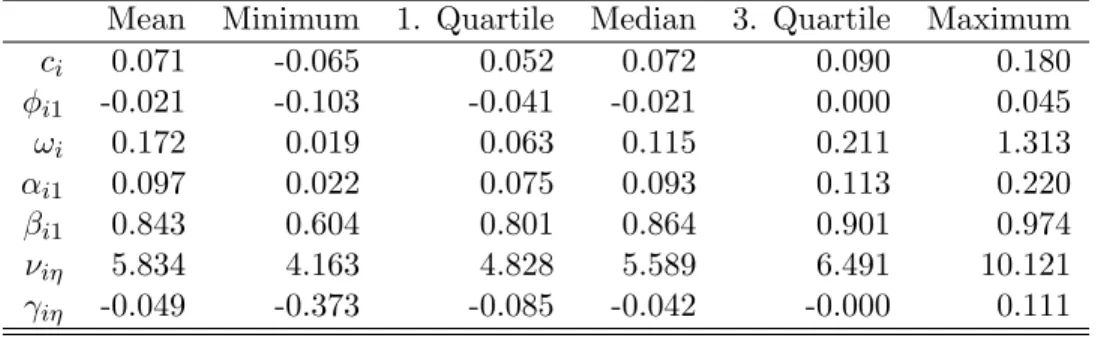
Table 2 shows the summary statistics for the posterior mean estimations of the univariate
AR(1)−GARCH(1,1) model across the 150 firms. The effect of conditional autoregressive mean is weak as the average value of φ1i is −0.021 and φ1i is insignificantly different from 0 in most of
marginals. This fact matches with other findings in the finance literature that the return levels are unpredictable. However, the variance returns are quite predictable through theGARCH(1,1) setting. The average ofαi1 and βi1 are significantly different from 0 for most of the marginals. On
average, the previous variance will contribute up to the 84% the value of the current variance which creates volatility clustering. The degrees of freedom for each marginal also diversifies between 4.2 and 10 which accounts for different kurtosis. The skewness parameter ranges from−0.373 to 0.111 and most of them are not significantly different from 0.
For the second stage, the standardized innovations are taken out and transformed to copula observations by applying the corresponding marginal cdfs. More specifically, using the posterior mean estimations for each marginal, we obtain the standardized innovations, ηit, of the AR(1)−
GARCH(1,1) process and transform them into the copula observationsuit =FGSt ηit|c¯i,φ¯1i,ω¯i,α¯1i,β¯1i,ν¯iη,γ¯iη
. This simplifies the computational burden in the high dimensional setting in which we only
con-centrate on estimating the copula parameters. Apart from that, we check if the choice of a GSt distribution is suitable with univariate GARCH volatilities by performing the Kolmogorov-Smirnov goodness of fit test. All series passed the test with p-values larger than 0.05. We also tested for
Table 2: Estimation results ofAR(1)−GARCH(1,1)-GSt for each marginal return
Mean Minimum 1. Quartile Median 3. Quartile Maximum
ci 0.071 -0.065 0.052 0.072 0.090 0.180 φi1 -0.021 -0.103 -0.041 -0.021 0.000 0.045 ωi 0.172 0.019 0.063 0.115 0.211 1.313 αi1 0.097 0.022 0.075 0.093 0.113 0.220 βi1 0.843 0.604 0.801 0.864 0.901 0.974 νiη 5.834 4.163 4.828 5.589 6.491 10.121 γiη -0.049 -0.373 -0.085 -0.042 -0.000 0.111
Summary statistics for the posterior mean estimations of the univariate AR(1) − GARCH(1,1)-GSt model across the 150 firms. The distribution of posterior mean es-timations are described by mean and quantiles.
serial correlation between the innovation and did not find significant results.
5.2 Copula estimation
Next, we apply the proposed Bayesian approach to nine different one factor copula models. These are the dynamic Gaussian, Student-t and MGSt combined with particular cases of models referred as block equivalent mean correlation, single group and multiple-group. In the block equi-mean correlation model, the parameter figc in (8) is restricted to be the same for the assets belonging
to the same group, i.e., f1gc = . . . = fnggc, for all g = 1, . . . , G. We classified G = 14 group
industries of assets depending on their SIC codes, as in Creal and Tsay (2015). These are Oil & Construction , Food & Beverage, Pharmaceuticals, Plastic Material & Plant Chemical, Textile & Papers, Steel, Home Appliances & Automobile, Electronics, Transportation, Telecommunication, Retail & Distribution, Insurance, Finance (not contained in Insurance), Services & Others. The detail number of firms are reported in Table 2 of Online Appendix. On average, there are 11 firms in each sector group. In the single group model, G= 1 as described in (5), only a few number of parameters account for tail dependence, while the correlations are allowed to be different across the assets. Finally, the multiple-group dynamic model is the most flexible one with different behaviours in tail and unrestricted correlation as in (8). In all cases, we generate 20.000 iterations with 10.000 burn-in for each factor copula model and every 10-th draws are taken in order to prevent the autocorrelation of the MCMC chains.
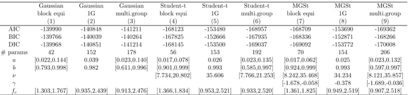
Table 3 outlines the main estimation results for the nine one factor copula models. In particular, the table includes the value of the AIC, BIC, and DIC model selection criteria, obtained as explained
Table 3: Estimation results for alternative copula models
Gaussian Gaussian Gaussian Student-t Student-t Student-t MGSt MGSt MGSt
block equi 1G multi.group block equi 1G multi.group block equi 1G multi.group
(1) (2) (3) (4) (5) (6) (7) (8) (9) AIC -139990 -140848 -141211 -168123 -153480 -168957 -168709 -153690 -169362 BIC -139766 -140039 -140264 -167825 -152666 -167935 -168336 -152871 -168266 DIC -139968 -140851 -141214 -168145 -153500 -169037 -169092 -153772 -170008 # params 42 152 178 56 153 192 70 154 206 a [0.022,0.144] 0.039 [0.023,0.140] [0.017,0.078] 0.026 [0.023,0.135] [0.017,0.062] 0.025 [0.023,0.132] b [0.793,0.998] 0.982 [0.611,0.996] [0.901,0.999] 0.993 [0.585,0.997] [0.924,0.999] 0.993 [0.597,0.997] ν [7.734,20.802] 35.606 [7.766,21.253] [8.242,35.468] 34.234 [8.121,35.857] γ [-1.678,-0.058] -0.378 [-1.689,-0.036] fc [1.303,1.767] [0.935,2.439] [0.913,2.476] [1.366,1.834] [0.953,2.521] [0.933,2.520] [1.361,1.825] [0.949,2.519] [0.907,2.518]
Posterior estimations for nine one factor copula models and model selection criteria. Three different models are considered (the block-equivalent, one group and multiple-group) for three different copula models (Gaussian, Student-t and MGSt). The table reports only the range of the posterior means for the group models and the point estimates for the one group model.
in Appendix C. The dynamic MGSt copula appears to show better fit over the Gaussian and Student-t copula models. In general, the posterior means of the parameters a,band fc are similar
across Gaussian, Student-t, and MGSt copulas, as shown for example in model (3), (6) and (9). The block equi-mean correlation model reports a smaller posterior range foraand b. The degrees of freedom and skewness parameters are roughly similar between the block-equivalent and the multiple-group models. The model selection criteria shows a interesting result that the models with more parameters accounting for extreme events are preferable over the models that have limitations on these behaviours. For example, in Gaussian copulas, the one group outperforms the block-equivalent due to the fact that they do not capture the extreme occurrences. However, it is preferable to use block equi-mean correlation in the Student-t and MGSt copulas rather than one group copula. The block-equivalent models could even be comparable with the multi-group models in all criteria AIC, BIC, and DIC. We also obtain that the group Student-t copula yields lower degrees of freedom than the single group Student-t copula. This finding confirms with Creal and Tsay (2015) due to the fact that when the number of assets in a group increases, the uncertainty reduces because the central limit theorem holds.
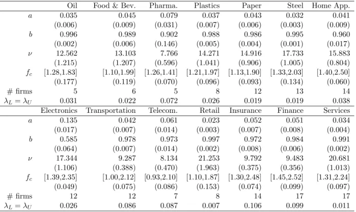
In Tables 4 and 5, we report respectively the detail estimations for the dynamic group
Student-t and dynamic group MGSStudent-t copulas. The posStudent-terior means of a and b shows different dynamic
behaviours in each group sector. The values of fc are depicted as interval range of the posterior
means of figc, for assets i = 1, . . . , ng belonging to each group g = 1, . . . , G. The values in
parentheses are the average values of the posterior standard deviations. The posterior means of ν
Table 4: Results for the group Student-t copula with time-varying factor loadings.
Oil Food & Bev. Pharma. Plastics Paper Steel Home App.
a 0.035 0.045 0.079 0.037 0.043 0.032 0.041 (0.006) (0.009) (0.031) (0.007) (0.006) (0.003) (0.009) b 0.996 0.989 0.902 0.988 0.986 0.995 0.960 (0.002) (0.006) (0.146) (0.005) (0.004) (0.001) (0.017) ν 12.562 13.103 7.766 14.271 14.916 17.733 15.883 (1.215) (1.207) (0.596) (1.041) (0.906) (1.005) (0.804) fc [1.28,1.83] [1.10,1.99] [1.26,1.41] [1.21,1.97] [1.13,1.90] [1.33,2.03] [1.40,2.50] (0.177) (0.119) (0.070) (0.096) (0.093) (0.134) (0.060) # firms 5 6 5 8 12 13 14 λL=λU 0.031 0.022 0.072 0.026 0.019 0.019 0.038
Electronics Transportation Telecom. Retail Insurance Finance Services
a 0.135 0.042 0.061 0.023 0.052 0.051 0.034 (0.017) (0.007) (0.014) (0.003) (0.007) (0.008) (0.004) b 0.585 0.978 0.973 0.997 0.972 0.984 0.991 (0.064) (0.007) (0.014) (0.002) (0.008) (0.006) (0.002) ν 17.344 9.287 8.134 21.253 9.792 9.483 20.681 (1.106) (0.388) (0.470) (1.963) (0.375) (0.356) (1.013) fc [1.39,2.35] [1.00,2.12] [0.93,2.10] [1.10,1.87] [1.30,2.48] [1.45,2.52] [1.31,2.24] (0.049) (0.075) (0.086) (0.153) (0.074) (0.099) (0.097) # firms 12 12 7 8 14 17 17 λL=λU 0.026 0.086 0.087 0.007 0.106 0.099 0.011
Posterior estimations for the interest parameters of the group Student-t factor copula. This includes the posterior means and standard deviations for (a, b, ν) and the values of fc are depicted as interval range of the posterior means together with the average posterior standard deviations. The tail dependences are calculated using bivariate Student-t copula with the mean correlation of the assets belonging to the same sector.
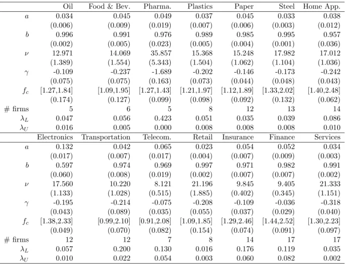
in the case of the group Student-t and seems to be higher in the MGSt model. The lowest degree of freedom parameter in the dynamic group Student-t is in Pharmaceutical industries standing at 7.8. However, in the MGSt copula model, it is strongly negative skewed which results in a higher posterior estimation for the degrees of freedom. While the other groups that have low degrees of freedom such as Telecommunication, Insurance, and Finance reveal a slight skewness. Although the posterior variation of the degrees of freedom in some industries are higher in the case of group MGSt copula, it still supports for the hypothesis that the lower tail is heavier and the distribution is highly asymmetric rather than there is a symmetry in both upper tail and lower tail. We show different tail dependences in each group sector by calculating the mean correlation of all assets in the groups and derive the upper tail and lower tail of bivariate MGSt copulas. The strongest lower tail dependence is 0.42 from the Pharmaceutical sector despite of no upper tail dependence.
Table 5: Results for the group MGSt copula with time-varying factor loadings.
Oil Food & Bev. Pharma. Plastics Paper Steel Home App.
a 0.034 0.045 0.049 0.037 0.045 0.033 0.038 (0.006) (0.009) (0.019) (0.007) (0.006) (0.003) (0.012) b 0.996 0.991 0.976 0.989 0.985 0.995 0.957 (0.002) (0.005) (0.023) (0.005) (0.004) (0.001) (0.036) ν 12.971 14.069 35.857 15.368 15.248 17.982 17.012 (1.389) (1.554) (5.343) (1.504) (1.062) (1.104) (1.036) γ -0.109 -0.237 -1.689 -0.202 -0.146 -0.173 -0.242 (0.075) (0.075) (0.163) (0.073) (0.044) (0.048) (0.043) fc [1.27,1.84] [1.09,1.95] [1.27,1.43] [1.21,1.97] [1.12,1.89] [1.33,2.02] [1.40,2.48] (0.174) (0.127) (0.099) (0.098) (0.092) (0.132) (0.062) # firms 5 6 5 8 12 13 14 λL 0.047 0.056 0.423 0.051 0.035 0.039 0.086 λU 0.016 0.005 0.000 0.008 0.008 0.008 0.010
Electronics Transportation Telecom. Retail Insurance Finance Services
a 0.132 0.042 0.065 0.023 0.054 0.052 0.034 (0.017) (0.007) (0.017) (0.004) (0.007) (0.009) (0.003) b 0.597 0.974 0.969 0.997 0.971 0.982 0.991 (0.060) (0.008) (0.019) (0.002) (0.007) (0.007) (0.002) ν 17.560 10.220 8.121 21.196 9.845 9.405 21.333 (1.133) (1.028) (0.515) (1.885) (0.402) (0.345) (1.151) γ -0.195 -0.214 -0.075 -0.208 -0.109 -0.036 -0.318 (0.043) (0.089) (0.035) (0.055) (0.037) (0.029) (0.040) fc [1.38,2.33] [0.99,2.10] [0.91,2.08] [1.09,1.85] [1.29,2.46] [1.44,2.52] [1.30,2.23] (0.049) (0.070) (0.082) (0.154) (0.074) (0.091) (0.097) # firms 12 12 7 8 14 17 17 λL 0.057 0.200 0.130 0.016 0.176 0.119 0.035 λU 0.010 0.022 0.054 0.003 0.060 0.082 0.002
Posterior estimations for the interest parameters of group MGSt factor copula. This includes the pos-terior means and standard deviations for (a, b, ν, γ) and the values of fc are depicted as interval range
of the posterior means together with the average posterior standard deviations. The tail dependence are calculated numerically using bivariate MGSt copula with the mean correlation of the assets belonging to the same sector (see Appendix A.4).
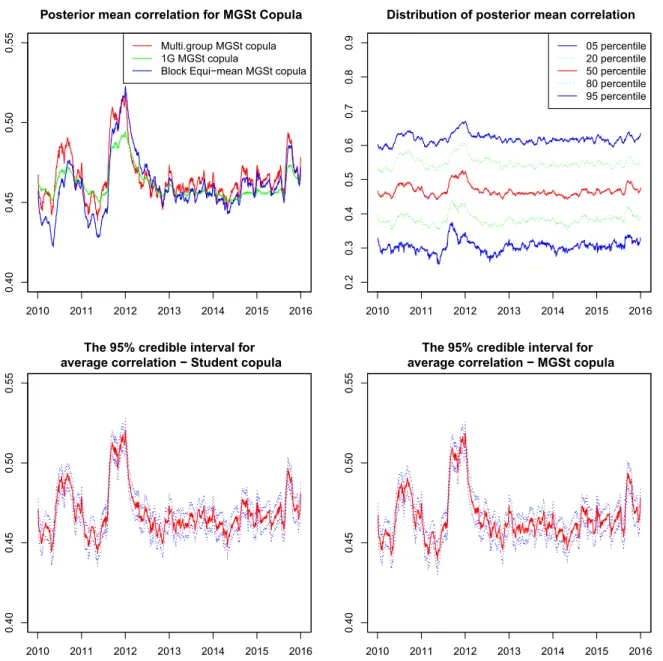
MGSt copula. This posterior mean is calculated as the average over iterations of the mean cor-relation between time series i and j as d(d−1)1 /2P
ijρitρjt where i, j = 1, . . . , d, i 6= j. In the top
left figure, we compare the mean correlation using block-equivalent, single group and multiple-group MGSt copula. The correlation path generated by block-equivalent model is close to that by multiple-group model, while the single group correlation path does not move much. Combined with the evidence of the model selection, we conclude that few parameters controlling for the dynamic behaviour of correlation is restrictive and the block equivalent mean correlation can approximate well the correlation structure in comparison to the multiple-group dynamic model. In the bottom left and bottom right figure, we illustrate the mean correlation together with the 95% credible interval of Student-t and MGSt copulas. They are almost the same in both point estimation as well as the confident brand. In the top right, we describe the distribution of mean correlationRijt
across the 150 time series. The one factor dynamic MGSt copula could capture different behaviour among the cross correlation. As we can see, a common pattern is that the correlation increased over time in the end of 2011. This finding is similar to Creal and Tsay (2015) for stochastic copula model because of the financial crisis in 2010−2011.
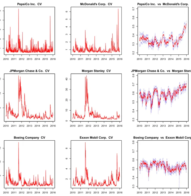
Figure 4 shows the posterior distribution of conditional variance and conditional correlation of several companies including PepsiCo, McDonalds, JP Morgan Chase, Morgan Stanley, Boeing, and Exxon Mobil using MGSt copula. The first two columns illustrate the conditional variance and the last column depicts the conditional correlation between the couple. As mentioned above, the 2010−2011 period experienced a high volatility and a rise in correlation among all examples due to the financial crisis. The cross correlation also goes up recently but not for every series which might be due to the shocks to separated sectors rather than the whole economy.
6
Conclusion
In this paper, we have proposed a family of one factor copula models and developed a Bayesian algorithm to make parallel inference on the model parameters. In our proposed models, the time series become independent conditioning on the latent factor that allows us to introduce an estima-tion strategy in a parallel setting. Furthermore, the factor loadings have been modelled as GAS processes which imposes a dynamic dependence structure in their densities. Using MGSt copulas,
2010 2011 2012 2013 2014 2015 2016
0.40
0.45
0.50
0.55
Posterior mean correlation for MGSt Copula
Multi.group MGSt copula 1G MGSt copula
Block Equi−mean MGSt copula
2010 2011 2012 2013 2014 2015 2016 0.2 0.3 0.4 0.5 0.6 0.7 0.8 0.9
Distribution of posterior mean correlation
05 percentile 20 percentile 50 percentile 80 percentile 95 percentile 2010 2011 2012 2013 2014 2015 2016 0.40 0.45 0.50 0.55
The 95% credible interval for average correlation − Student copula
2010 2011 2012 2013 2014 2015 2016
0.40
0.45
0.50
0.55
The 95% credible interval for average correlation − MGSt copula
Figure 3: The distribution of posterior correlation among factor copula models
The mean correlation using block equi-mean correlation, single group and multiple-group MGSt copula shown in the top left. The top right figure shows the distribution of mean correlation across 150 time series. The two bottom figures illustrate the mean correlation together with the 95% credible interval of multiple-group Student and MGSt copula.
2010 2011 2012 2013 2014 2015 2016 1 2 3 4 5 PepsiCo Inc. CV 2010 2011 2012 2013 2014 2015 2016 1 2 3 4 5 6 McDonald's Corp. CV 2010 2011 2012 2013 2014 2015 2016 0.2 0.3 0.4 0.5 0.6 0.7
PepsiCo Inc. vs McDonald's Corp.
2010 2011 2012 2013 2014 2015 2016
5
10
15
JPMorgan Chase & Co. CV
2010 2011 2012 2013 2014 2015 2016 0 10 20 30 40 Morgan Stanley CV 2010 2011 2012 2013 2014 2015 2016 0.3 0.4 0.5 0.6 0.7 0.8
JPMorgan Chase & Co. vs Morgan Stanley
2010 2011 2012 2013 2014 2015 2016 5 10 15 Boeing Company CV 2010 2011 2012 2013 2014 2015 2016 2 4 6 8
Exxon Mobil Corp. CV
2010 2011 2012 2013 2014 2015 2016 0.3 0.4 0.5 0.6 0.7 0.8
Boeing Company vs Exxon Mobil Corp.
Figure 4: Posterior correlation among each time series
The first two columns describe the conditional variance and the last column depicts the conditional correlation together with the 95% credible interval using MGSt copula. First row: PepsiCo, McDonald, second row: JP Morgan Chase, Morgan Stanley, third row: Boeing, Exxon Mobil
we obtain different types of tail and asymmetric dependence. The models are extendible since the number of parameters scales linearly with the dimension. As extension, more complex copula functions can be build based on the distribution of ζg. However, this also may require more
com-putational cost to obtain the inverse cdf. Also, we might consider factor models using the family of Archimedean copulas, whose have only lower tail dependence, due to the empirical finding that half of the groups only show weak evidence of upper tail dependence. Finally, one factor models may not be enough for the high dimensional dependence as Oh and Patton (2017a) suggest. One future direction could be to extend the proposed approach to dynamic multi factor models.
Appendix
A
Score update for one factor copula model
A.1 Dynamic Gaussian one factor copula
The conditional cdf of ut= (u1t, . . . , udt)0, whereuit = Φ (xit),is:
F(u1t, . . . , udt|zt, ft,Ft, θ) = Pr (U1t≤u1t, . . . , Udt≤udt|zt, ft,Ft, θ) = Pr X1t≤Φ−1(u1t), . . . , Xdt ≤Φ−1(udt)|zt, ft,Ft, θ = d Q i=1 Pr Xit≤Φ−1(uit)|zt, ft,Ft, θ .
Note that, given{zt, ft,Ft, θ}, the correlationρit is known andXitfollows a Gaussian distribution
with mean ρitztand standard deviation
q
1−ρ2it. Then, the conditional density of ut is,
p(ut|zt, ft,Ft, θ) = ∂dF(u1t, . . . , udt|zt, ft,Ft, θ) ∂u1t. . . ∂udt = d Q i=1 φ Φ−1(uit)|ρitzt, q 1−ρ2it φ(Φ−1(u it)|0,1) ,
whereφ(· |µ, σ) denotes a normal pdf with mean,µ, and standard deviation,σ. Then, the proposed dynamic process is based on the derivative of the log conditional density wrt the dynamicfit,
sit = ∂logp(ut|zt, ft,Ft, θ) ∂fit = ∂logp(ut|zt, ft,Ft, θ) ∂ρit ∂ρit ∂fit = ∂ d P i=1 logφ Φ−1(uit)|ρitzt, q 1−ρ2it −logφ Φ−1(uit)|0,1 ∂ρit 1−ρ2it 2 = ∂−12log(2π)−12log(1−ρ2 it)− 12 (Φ−1(u it)−ρitzt)2 1−ρ2 it ∂ρit 1−ρ2it 2 = ρit (1−ρ2 it) +zt(Φ −1(u it)−ρitzt) 1−ρ2 it −ρit(Φ −1(u it)−ρitzt)2 (1−ρ2 it)2 1−ρ2it 2 = 1 2Φ −1(u it)zt+ 1 2ρit−ρit Φ−1(uit)2+zt2−2ρitΦ−1(uit)zt 2(1−ρ2it) ,
A.2 Dynamic Student one factor copulas
The conditional cdf of ut= (u1t, . . . , udt), where uit=FSt(xit |ν),is:
F(u1t, . . . , udt |zt, ζt, ft,Ft, θ) = Pr X1t≤FSt−1(u1t|ν), . . . , Xdt≤FSt−1(udt|ν)|zt, ζt, , ft,Ft, θ = d Q i=1 Pr X˙it ≤ FSt−1√(uit|ν) ζt |zt, ζt, ft,Ft, θ ! , where ˙Xit =Xit/ √
ζt.Similarly, given{zt, ζt, ft,Ft, θ},the correlationρitis known and ˙Xit follows
a Gaussian distribution with mean ρitzt and standard deviation
q
1−ρ2
it. Then, the conditional
density ofut is, p(ut|zt, ζt, ft,Ft, θ) = ∂dF(u1t, . . . , udt|zt, ζt, ft,Ft, θ) ∂u1t. . . ∂udt = d Q i=1 φ F−1 St√(uit|ν) ζt |ρitzt, q 1−ρ2it fSt FSt−1(uit|ν)|ν √ ζt ,
wherefSt(· |ν) denotes the standard Student-t with ν degrees of freedom. Thus, the equation for
sit remains, sit= ∂logp(ut|zt, ζt, ft,Ft, θ) ∂fit = ∂logφ F−1 St√(uit|ν) ζt |ρitzt, q 1−ρ2it ∂ρit 1−ρ2it 2 = 1 2 FSt−1√(uit |ν) ζt zt+ 1 2ρit−ρit F−1 St√(uit|ν) ζt 2 +zt2−2ρit FSt−1√(uit|ν) ζt zt 2(1−ρ2 it) ,
which leads to the expression given in (4).
A.3 Dynamic hyperbolic skew Student one factor copula
The conditional cdf of ut= (u1t, . . . , udt), where uit=FGSt(xit|ν, γ),is:
F(u1t, . . . , udt|zt, ζt, ft,Ft, θ) = Pr X1t≤FGSt−1 (u1t|ν, γ), . . . , Xdt ≤FGSt−1 (udt |ν, γ)|zt, ζt, ft,Ft, θ = d Q i=1 Pr X˜it≤ FGSt−1 (uit |ν, γ)−γζt √ ζt |zt, ζt, ft,Ft, θ ! , where ˜Xit = (Xit−γζt)/ √
ζt. Similarly, given {zt, ζt, ft,Ft, θ}, the correlation ρit is known and
˙
Xit follows a Gaussian distribution with meanρitzt and standard deviation
q
conditional density of ut is, p(ut|zt, ζt, ft,Ft, θ) = ∂dF(u1t, . . . , udt|zt, ζt, ft,Ft, θ) ∂u1t. . . ∂udt = d Q i=1 φF −1 GSt(u√it|ν)−γζt ζt |ρitzt, q 1−ρ2it fGSt FGSt−1 (uit|ν, γ)|ν, γ √ ζt , (10) where fGSt(· |ν, γ) denotes the standard generalized hyperbolic skew Student-t with ν degrees of
freedom andγ skewness parameter. Thus, the equation forsit remains,
sit= ∂logp(ut|zt, ζt, ft,Ft, θ) ∂fit = ∂logφF −1 GSt(u√it|ν)−γζt ζt |ρitzt, q 1−ρ2 it ∂ρit 1−ρ2it 2 = 1 2 FGSt−1 (uit|ν)−γζt √ ζt zt+ 1 2ρit−ρit F−1 GSt(u√it|ν)−γζt ζt 2 +z2t −2ρit FGSt−1(u√it|ν)−γζt ζt zt 2(1−ρ2it) ,
which leads to the expression given in (6).
A.4 Tail dependence for hyperbolic skew Student copula
Consider the bivariate MGSt copula. We derive the tail dependence of a pair of pseudo observables
xigt and xjtg in a same group,g, from the Equation (7) as:
xigt =γgζg+ p ζg ρigtzt+ q 1−ρ2igtigt xjgt=γgζg+ p ζg ρjgtzt+ q 1−ρ2 jgtjgt (11)
Demarta and McNeil (2005) suggest that the joint quantile exceedance probability is obtained as the integral over the nuisance parameters (zt, ζgt),
C(u, u|νg, γg) = Pr(xigt ≤FGSt−1(u), xjgt≤FGSt−1 (u)) =E Pr igt ≤ FGSt−1(u)−γgζgt p ζgt q 1−ρ2igt −qρigtzt 1−ρ2igt , jgt≤ FGSt−1 (u)−γgζgt p ζgt q 1−ρ2jgt −qρjgtzt 1−ρ2jgt =E Φ FGSt−1 (u)−γgζgt p ζgt q 1−ρ2igt −qρigtzt 1−ρ2igt Φ FGSt−1 (u)−γgζgt p ζgt q 1−ρ2jgt −qρjgtzt 1−ρ2jgt (12)
Then, we obtainC(u, u|νg, γg) as the numerical integral overzt∼N(0,1) andζgt∼IG(νg/2, νg/2)
As taking the equation to the limit, the tail dependence are,
λL= lim u→0 C(u, u|νg, γg) u λU = 2 + lim u→0 C(1−u,1−u|νg, γg)−1 u
Table (5) reports the tail dependence of bivariate MGSt copula atu= 0.005.
B
Posterior inference
From the joint posterior of the dynamic hyperbolic skew Student factor copula model in (9), we derive the conditional posterior for each parameters as follows:
p(zt|u, a, b, fc, ν, γ, ζ)∝ G Y g=1 ng Y i=1 φ(˜xigt |ρigtzt, q 1−ρ2 igt)φ(zt|0,1) p(figc|u, a, b, z, ν, γ, ζ)∝ T Y t=1 ng Y i=1 φ(˜xigt |ρigtzt, q 1−ρ2igt) p(ag|u, b, f, z, ν, γ, ζ)∝ T Y t=1 ng Y i=1 φ(˜xigt |ρigtzt, q 1−ρ2igt) p(bg|u, a, f, z, ν, γ, ζ)∝ T Y t=1 ng Y i=1 φ(˜xigt |ρigtzt, q 1−ρ2igt) p(νg|u, f, a, b, z, γ, ζ)∝ T Y t=1 ng Y i=1 φ(˜xigt |ρigtzt, q 1−ρ2 igt) fGSt(xigt|νg, γg) × T Y t=1 IGζgt| νg 2 , νg 2 G(νg−4|2,2.5) p(γg|u, f, a, b, z, ν, ζ)∝ T Y t=1 ng Y i=1 φ(˜xigt |ρigtzt, q 1−ρ2 igt) fGSt(xigt|νg, γg) φ(γg|0,1) p(ζgt|u, f, a, b, z, ν, γ)∝ ng Y i=1 φ(˜xigt|ρigtzt, q 1−ρ2 igt) p ζgt IG ζgt | νg 2 , νg 2
As the conditional posterior of zt only depends on the pseudo observations at time t, we can
make parallel inference for t= 1, . . . , T. Also, the conditional posteriors of ag, bg, νg, γg and ζgt
g = 1, . . . , G. Finally, conditional on zt, each time series is independent, for i = 1, . . . , ng and
g= 1, . . . , G. Then, we also create a parallel estimation procedure forfigc.
C
Model selection
The statistics of model selection are calculated based on the average of the log-likelihood. We take the average of the log likelihood after MCMC iterations at the posterior mean of the interested parameters as the integral over the nuisance parameter space. The set parameters of interest is
θint={a, b, fc, ν, γ}and the nuisance parameters areθnui ={z, ζ}.
AIC =−2Eθnui log p u|θ¯int, f,F + 2k BIC =−2Eθnui log p u|θ¯int, f,F +klogT DIC =−4Eθ[logp(u|θ, f,F)|u] + 2Eθnui
log p u|θ¯int, f,F