ScholarWorks
Mathematics Faculty Publications and Presentations
Department of Mathematics
1-1-2017
A Radial Basis Function (RBF) Compact Finite
Difference (FD) Scheme for Reaction-Diffusion
Equations on Surfaces
Erik Lehto
KTH Royal Institute of Technology
Varun Shankar
University of Utah
Grady B. Wright
Boise State UniversityFirst published inSIAM Journal on Scientific Computing 39(5), published by the Society of Industrial and Applied Mathematics (SIAM). Copyright © by SIAM. Unauthorized reproduction of this article is prohibited.
A RADIAL BASIS FUNCTION (RBF) COMPACT FINITE DIFFERENCE (FD) SCHEME FOR REACTION-DIFFUSION
EQUATIONS ON SURFACES∗
ERIK LEHTO†, VARUN SHANKAR‡, AND GRADY B. WRIGHT§
Abstract. We present a new high-order, local meshfree method for numerically solving reaction diffusion equations on smooth surfaces of codimension 1 embedded inRd. The novelty of the method
is in the approximation of the Laplace–Beltrami operator for a given surface using Hermite radial basis function (RBF) interpolation over local node sets on the surface. This leads to compact (or implicit) RBF generated finite difference (RBF-FD) formulas for the Laplace–Beltrami operator, which gives rise to sparse differentiation matrices. The method only requires a set of (scattered) nodes on the surface and an approximation to the surface normal vectors at these nodes. Additionally, the method is based on Cartesian coordinates and thus does not suffer from any coordinate singularities. We also present an algorithm for selecting the nodes used to construct the compact RBF-FD formulas that can guarantee the resulting differentiation matrices have desirable stability properties. The improved accuracy and computational cost that can be achieved with this method over the standard (explicit) RBF-FD method are demonstrated with a series of numerical examples. We also illustrate the flexibility and general applicability of the method by solving two different reaction-diffusion equations on surfaces that are defined implicitly and only by point clouds.
Key words. RBF-FD, RBF-HFD, manifolds, reaction diffusion AMS subject classifications. 41A21, 65D05, 65E05, 65F22 DOI. 10.1137/16M1095457
1. Introduction. Global radial basis function (RBF) methods are quite popular for the numerical solution of various partial differential equations (PDEs) due to their ability to handle scattered node layouts, their simplicity of implementation, and their potential for spectral accuracy for smooth problems. These methods have been successfully applied to the solution of PDEs in various geometries inR2and
R3(e.g.,
[12, 17]), including spherical domains (e.g., [27, 16, 42]), and more general surfaces embedded inR3(e.g., [26, 36]).
When high orders of algebraic accuracy are sufficient for a given problem, or if the solutions to the problem are expected to only have finite smoothness, RBF generated finite difference (RBF-FD) formulas are an attractive alternative to global RBFs as they perform better in terms of accuracy per computational cost [17]. These formulas are generated from RBF interpolation overlocal sets of nodes (stencils) so that the resulting differentiation matrices are sparse as in the standard FD method. In contrast to standard FD methods, however, the RBF-FD method can naturally handle irregular geometries and scattered node layouts. Additionally, their locality
∗Submitted to the journal’s Methods and Algorithms for Scientific Computing section September
23, 2016; accepted for publication (in revised form) March 27, 2017; published electronically Septem-ber 21, 2017.
http://www.siam.org/journals/sisc/39-5/M109545.html
Funding: The work of the second author was supported by this project under NSF-DMS 1160432. The work of the third author was funded by support for this project under grants NSF-DMS 1160379 and NSF-ACI 1440638.
†Corresponding author. Department of Mathematics, KTH Royal Institute of Technology,
Stock-holm, 10044, Sweden ([email protected]).
‡Department of Mathematics, University of Utah, Salt Lake City, UT 84112 (vshankar@math.
utah.edu).
§Department of Mathematics, Boise State University, Boise, ID 837235 (gradywright@
makes them more flexibility in terms of local refinement strategies than global RBF methods. The strength of the RBF-FD method has been leveraged to solve problems on planar domains, e.g., [39, 6, 43, 7, 40], the surface of a sphere [19, 15], and, more recently, very general surfaces represented solely by point clouds and normal vectors [38].
It is natural to view these two classes of RBF methods as extensions of classical methods to scattered nodes and irregular geometries. The global RBF method for surface PDEs in [26] may be viewed as an extension of polynomial based (or Fourier based) pseudospectral methods to surfaces, while the RBF-FD method presented in [38] may be viewed as an extension of standard, polynomial based FD methods to surfaces. In this work, we turn our attention to the extension of a third important class of classical methods to surfaces: the so-called compact, implicit, or Hermite FD methods, first introduced by Collatz [9]. We use the acronym HFD for these schemes to avoid the obvious confusion with CFD, and because they will ultimately be based on Hermite interpolation.
The goal of HFD methods is to solve a given PDE numerically by computing more accurate approximations to the differential operators in the PDE. In these schemes, this improved accuracy is obtained by using additional information from the PDE itself, rather than increasing the stencil size, as is the usual way to increase the ac-curacy with standard (or explicit) FD methods. HFD schemes are thus typically more computationally efficient than standard FD schemes, as they can obtain higher accuracy and resolution for the same stencil size [31]. Further, the differentiation matrices obtained from HFD formulas often have desirable properties such as diago-nal dominance, leading to both enhanced numerical stability and faster convergence of iterative methods used in solving the sparse linear systems that arise when using these matrices to discretize a PDE. While HFD schemes have already been success-fully generalized to scattered node layouts [43], the application of these schemes to the solution of PDEs on surfaces presents significant challenges due to the presence of surface differential operators. In this article, we overcome those challenges and present a new RBF-HFD scheme for the solution of reaction-diffusion equations on surfaces.1 The resulting method uses Cartesian coordinates, thereby avoiding the
singularities typically associated with intrinsic coordinate systems. Further, our new method only uses nodes on the surface in consideration, making it more computation-ally efficient than embedded narrow-band methods that solve the PDE in a narrow band in the embedding space (e.g., [32, 36]). Finally, the RBF-HFD formulas require fewer nodes than the RBF-FD method presented in [38] for the same accuracy, while also possessing improved stability properties.
The remainder of the paper is organized as follows. In section 2, we briefly review the formulation of surface differential operators in Cartesian coordinates. Section 3 outlines Hermite RBF interpolation on scattered node sets inRd. Section 4 describes
how to use approximations to the Hermite RBF interpolants to generate RBF-HFD weights for approximating the surface Laplacian, and also how these can be arranged intosparsedifferentiation matrices. We follow this in section 5 with a brief discussion of how to use these differentiation matrices in a method-of-lines formulation for nu-merically solving forced diffusion equations on surfaces. In section 6, we discuss the stability of our method by studying the Gershgorin sets associated with the eigen-values of our differentiation matrices. In section 7, we numerically demonstrate the
1Throughout this paper, we will use the terms surface or manifold to refer to embedded
accuracy and efficiency of our method for the forced scalar diffusion equation on two different surfaces. We also present a few applications of our method to two species re-action diffusion equations on implicitly defined surfaces and surfaces defined by point clouds, which have relevant biological applications. We conclude our paper with a summary and discussion of future research directions in section 8.
2. Review of differential geometry. While the standard way of expressing differential operators on surfaces is through the use of intrinsic coordinates, covari-ant derivatives and metric tensors [5], we instead choose to formulate these operators entirely in Cartesian (or extrinsic) coordinates, as this avoids any singularities asso-ciated with intrinsic coordinate systems. Consider the standard gradient operator in
R3, ∇ =∂x ∂y ∂z T
. If we apply this to a differentiable functionf at a point x= (x, y, z) on the surfaceMand then project the resulting vector into the tangent space of the surface, then this gives the surface gradient of f, which we denote as
∇Mf. Mathematically, this can be accomplished as follows. Letn=
nx ny nzT
be theunit normal vector toMat x; then
∇Mf =∇f −n(n· ∇f) =∇f−nnT(∇f).
Thus, the surface gradient operator can written entirely in Cartesian coordinates as
∇M:=∇ −nnT∇= (I −nnT)
| {z }
P ∇,
whereI is the 3-by-3 identity matrix. P is aprojection operator that takes a vector field inR3sampled at a pointxon the surface and projects it onto the tangent plane
to the surface atx. An explicit expression for this operator is given by
P = (1−nxnx) −nxny −nxnz −nxny (1−nyny) −nynz −nxnz −nynz (1−nznz) = px py pz , (1)
where px, py, and pz are vectors representing the projection operators in the x, y,
andz directions, respectively. We can now usepx,py, andpz to obtain the following
(more convenient) expression for∇M:
∇M:=P∇= px· ∇ py· ∇ pz· ∇ = Gx Gy Gz , (2)
where Gx, Gy, and Gz are the components of the surface gradient along each of the
coordinate directions in R3. Now, the surface Laplace (Laplace–Beltrami) operator
∆M can be obtained by applying the surface divergence to the surface gradient [26]. This can naturally be expressed usingGx,Gy, andGz as
∆M:=∇M· ∇M= (P∇)·(P∇) =GxGx+GyGy+GzGz.
(3)
This gives an explicit expression for the surface Laplace operator entirely in Cartesian components. We will use this expression in our numerical approximation to the surface Laplacian.
3. Hermite Interpolation with RBFs. We now review Hermite interpolation with RBFs, a technique essential to deriving the new RBF-HFD scheme outlined in the next section. Let Ω⊆Rdand letφ:Rd×Rd →Rbe a scalar-valued radial kernel,
i.e., φ(x,y) :=φ(kx−yk) for x,y ∈Ω, where k · kis the standard Euclidean norm inRd. LetLbe a linear functional and suppose we are given samples of a continuous
target function f at a set of distinct nodes X ={xi}ni=1 ⊂Ω and samples of Lf at
a set of distinct nodes ˜X = {x˜j}mj=1 ⊂Ω. Then we consider the following Hermite
RBF interpolant to the this data, proposed first by Wu [44]:
Iφf(x) = n X i=1 ciφ(x,xi) + m X j=1 djL2φ(x,x˜j) +α. (4)
Here we have used the notationL2 to mean thatLis applied toφwith respect to its
second argument. Later we will similarly useL1 to mean thatLis applied to φwith
respect to its first argument. The expansion coefficients {ci}ni=1 and {dj}mj=1 in (4)
are determined by enforcing the (Hermite) interpolation conditions
Iφf|X= f|X,
(5)
L(Iφf)|X˜ = (Lf)|X˜,
(6)
while the constant α is obtained by enforcing the moment condition Pni=1ci = 0.
These conditions can be represented as the following block linear system:
A B2 e B1 C 0 eT 0T 0 | {z } AH c d α = f Lf 0 , (7) where Ai,j =φ(xi,xj), i, j= 1, . . . , n, (B2)i,j =L2φ(xi,x˜j), i= 1, . . . , n, j= 1, . . . , m, (B1)i,j =L1φ(˜xi,xj), i= 1, . . . , m, j= 1, . . . , n, Ci,j =L1L2φ(˜xi,x˜j), i, j= 1, . . . , m, ei = 1, i= 1, . . . , n.
Becauseφis radially symmetric, we have thatφ(x,x˜) =φ(˜x,x), so thatL2φ(x,x˜) =
L1φ(˜x,x). This means thatA=AT, C=CT, andB2=B1T so that the matrixAH
is symmetric. Ifφ is, for example, positive definite or order-1 conditionally positive definite, then under very mild conditions on L the linear system (7) is nonsingular [44, 33].
We will also make use of regular RBF interpolation, which consists only of in-terpolating function values, in the subsequent section. These interpolants are simply given by (4) withmset equal to zero and the constantαomitted, i.e.,
Iφf(x) = n X i=1 ciφ(x,xi). (8)
In this case, we only enforce the conditions (5), which can be represented by the linear system
whereARis the same matrix asAin (7). We use the subscript R to denote the linear
system for theregular interpolant as opposed to the subscript H in (7) for the linear system associated with theHermite interpolant.
In this study, the interpolation nodes X and “functional nodes” ˜X lie on an embedded lower dimensional surface Ω = M in Rd. However, we will still use the
standard Euclidean distance in Rd for computingφ(x,x˜) = φ(kx−˜xk) in (4) (i.e.,
straight line distances rather than distances intrinsic to the surface). A theoretical foundation for RBF interpolation on surfaces with the straight-line distance measure is given in [24], along with proofs of favorable error estimates.
While it is possible to use any (conditionally) positive-definite kernel within the RBF-FD and RBF-HFD methods (e.g., [39, 43, 4, 10, 15]), we use the Gaussian (GA) kernel, which is positive definite inRdfor anyd. All infinitely smooth kernels feature
a shape parameterεsuch that large values ofεmake the kernels peaked, while smaller
ε values make them flat. In the limit asε→0, Gaussian RBF interpolants to data converge to (multivariate) polynomial interpolants inRd[11, 29, 37], and to spherical
harmonic interpolants on the sphereS2 [21]. While smaller values ofεgenerally lead
to greater accuracy for smooth target functions [22, 29], the interpolation matrix in (7) becomes increasingly ill-conditioned asε→0 (see, e.g., [23]). Some stable algorithms have been developed for bypassing this ill-conditioning [22, 21, 13, 18, 20], but these algorithms typically break down when the data sites lie on a submanifoldM⊂Rd, as
in the present study, due to nodes being nonunisolvent with respect to polynomials in
Rd. While some strategies have recently been undertaken to resolve them inRd [30],
a robust approach is not yet available for surfaces.
4. RBF-HFD formulas for the surface Laplacian. Let Ξ ={ξk}N
k=1denote
a set of (scattered) node locations on a surface M of dimension 2 embedded in R3
and suppose f : M → R is some differentiable function sampled on Ξ. Our goal is to approximate ∆Mf|Ξ with HFD-style local approximations to the operator ∆M. Without loss of generality, let the node where we want to approximate ∆Mf at be
ξ1, and let ξ2, . . . ,ξp be the p−1 nearest neighbors toξ1, measured by Euclidean distance inR3. We refer toξ1and itsp−1 nearest neighbors as the neighborhood of ξ1 on the surface and denote this neighborhood as S1={ξ`}
p
`=1; this neighborhood
will comprise the candidate nodes that make up the HFD stencil forξ1. We seek an approximation to ∆Mf atξ1that involves a linear combination of the values off and ∆Mf over some subset of nodes fromS1of the form
(10) (∆Mf)x=ξ 1 ≈X i∈J wif(ξi) + X j∈J˜ ˜ wj(∆Mf) x=ξ j ,
whereJ and ˜J denote index sets of sizen≤pandm < p, respectively, intoS1for the
explicit and the implicit (or Hermite) part of the stencil, respectively. We will assume that 1∈J, but 1∈/J˜(otherwise a trivial solution would exist). Using the notation of the previous section, we will let thennodes indicated byJbe denoted byX ={xi}ni=1
and themnodes indicated by ˜J be denoted by ˜X ={x˜j}mj=1. Additionally, we always
setx1=ξ1. Using this notation we can rewrite (10) as
(11) (∆Mf)x=x 1 ≈ n X i=1 wif(xi) + m X j=1 ˜ wj(∆Mf) x=˜x j.
The weights{wi}ni=1and{w˜j}mj=1in this approximation will be computed using RBFs,
4.1. Computation of the weights from the Hermite interpolant. The method from [43] determines the RBF-HFD weights in (11) from the Hermite RBF interpolant (4) constructed with L = ∆M. To compute the weights, consider the problem of applying ∆Mto the interpolant (4) and evaluating it atx1to approximate
∆Mfx=x
1. The resulting approximation would be exact whenever f is any of the
functionsφ(x,xi),i= 1, . . . , n,L2φ(x,x˜j) = ∆M,2φ(x,x˜j),j= 1, . . . , m, or a nonzero
constant (since the interpolant is exact for thesef). Thus, the weights{wi}ni=1 and
{w˜j}mj=1are the values that make (11) exact for these values off. This can be written
as the following linear system:
(12) A B e BT C 0 eT 0T 0 | {z } AH w ˜ w α = ∆M,1φ(x,xi) x=x1 ∆M,1∆M,2φ(x,x˜j) x=x 1 0 ,
where the block matricesAandC are the same as those given in the Hermite inter-polation matrix (7),B =B2=BT1 in this same matrix (recall that the matrix in (7)
is symmetric), ∆M,1=L1 and ∆M,2=L2, and i= 1, . . . , nandj= 1, . . . , m to form
block vectors of length nand min the right-hand side. Note that the constantαis not used for anything in the actual RBF-HFD formula.
The issue with using (12) for determining the RBF-FD weights is that one has to explicitly compute ∆M,1φ(x,x˜j) and ∆M,1∆M,2φ(x,x˜j). As discussed in section 2,
constructing ∆M requires having explicit information about the underlying surface, such as an analytical expression for the surface normal vectors. Even in cases where these are known, the resulting formulas for computing ∆M,1φ and ∆M,1∆M,2φ are
likely to be quite complex. Moreover, we are interested in surfaces that are defined by point clouds and where only numerical representations of the normal vectors are available. Thus, constructing the system (12) analytically will not be possible. How-ever, it is possible to construct an approximation to the entries of this system using the regular RBF-FD method from [38], which is based on iterated differentiation (see also [25]). This is the approach we take.
4.2. Computation of the weights from iterated differentiation. The first goal is to compute approximations of the entries inBT in (12) and the entries of the
first vector block in the right-hand side of this equation. We state the entries ofBT
explicitly as it will help elucidate the discussion of their approximation:
BT = ∆M,1φ(˜x1,x1) · · · ∆M,1φ(˜x1,xn) .. . . .. ... ∆M,1φ(˜xm,x1) · · · ∆M,1φ(˜xm,xn) . (13)
We compute these approximations by constructing an approximation to ∆M using discrete approximations toGx, Gy, andGz in (2) computed from the standard RBF
interpolant (8) over the candidate stencil nodesS1={ξk} p
k=1. To this end, consider,
for example, applyingGxto the interpolantI
φf in (8) based on the nodes inS1(here
the target functionf is not important) and then evaluating it atS1:
(GxI φf(x)) x=ξ i = p X j=1 cj Gxφ(x,ξj) x=ξ i | {z } Dxij , i= 1, . . . , p. (14)
We can rewrite (14) so that it explicitly depends only on the vector of samples fS 1 using (9) as follows: (15) (GxI φf) S 1 =D xc f =DxA−R1f S 1 =:G xf S 1.
HereGxis ap-by-pdifferentiation matrix that represents the RBF approximation to
thexcomponent of the surface gradient operator over the set of nodes in S1. Now,
letting Dyi,j= Gyφ(x,ξ j) x=ξ i and Di,jz = Gzφ(x,ξ j) x=ξ i , i, j= 1, . . . , p, (16)
we can obtain similar approximations to they and zcomponents of the surface gra-dient operator onS1 as (GyI φf) S 1=D yA−1 R f S 1=:G yf S 1, (17) (GzI φf) S 1=D zA−1 R f S 1 =:G zf S 1. (18)
To obtain an approximation to ∆M at the candidate stencil nodesS1, we mimic
the continuous formulation of the surface Laplacian in (3), replacing the continuous operators Gx, Gy, and Gz with the differentiation matrices Gx, Gy, and Gz,
respec-tively. This gives the following differentiation matrix for approximating the surface Laplacian at the nodesS1:
LM,1=GxGx+GyGy+GzGz = DxA−R1Dx+DyAR−1Dy+DzA−R1Dz | {z } ˆ BT A−R1. (19)
When applyingLM,1to a vector of samples of a target functionf taken overS1, this
is equivalent to interpolating the target function with the regular RBF interpolant (8), computing the components of the surface gradient of the interpolant, then inter-polating each of these components again using (8), applying the surface divergence, then evaluating this at the nodes inS1. This is a type of iterated derivative
approxi-mation [25] and has the advantage of not needing the explicit formulas for the normal vectors (or their derivatives) to the surfaceM.
Recall that the node sets X and ˜X are subsets ofS1 given by the index sets J
and ˜J, respectively (cf. (10)). Thus, to approximate the (i, `) entry, ∆M,1φ(˜xi,x`),
ofBT in (13), we can first applyL
M,1to the vector of samples ofφ(x,x`) atS1,
φ(ξ1,x`) φ(ξ2,x`) · · · φ(ξp,x`) T
,
(20)
which gives a vector containing approximations to ∆M,1φ(ξk,x`), k= 1, . . . , p. The
approximation to ∆M,1φ(˜xi,x`) is then given by the row in this vector corresponding
to theith value in ˜J (which we denote by ˜Ji). Note, however, that the vector (20) is
just theJ`column ofARin (15), so that the approximation to ∆M,1φ(˜xi,x`) obtained
from applyingLM,1to (20) is just given by the ˜JiandJ`column of ˆBT in (19). Thus,
all entries inBT in (13) can be similarly obtained directly from the rows and columns
or ˆBT using the index setsJ and ˜J. Additionally, the vector in the first block of the
right hand side of (12) can be approximated from ˆBT; in this case, from the first row
of ˆBT and from the columns corresponding toJ
The second goal is to compute approximations to the entries ofCin (12) and the entries of the second vector block in the right-hand side of this equation. We give the entries ofC explicitly to again elucidate the discussion:
C= ∆M,1∆M,2φ(˜x1,x˜1) · · · ∆M,1∆M,2φ(˜x1,x˜m) .. . . .. ... ∆M,1∆M,2φ(˜xm,x˜1) · · · ∆M,1∆M,2φ(˜xm,x˜m) . (21)
To approximate the operator ∆M,1∆M,2 we again use iterated differentiation
involv-ing the differentiation matrices Gx, Gy, and Gz. Using the idea of (19), we can
approximate ∆M,2 at the candidate stencil nodesS1using the differentiation matrix LM,2= (Dx)TAR−1(Dx)T+ (Dy)TA−R1(Dy)T + (Dz)TA−R1(Dz)T | {z } ˆ B A−R1, (22)
whereDx,Dy, andDz are given by (14) and (16). We then approximate ∆
M,1∆M,2 at the nodes inS1as LM,1LM,2= ˆ BTA−R1Bˆ | {z } ˆ C A−R1. (23)
Using similar arguments as above for extracting approximations to the elements ofBT
from ˆBT, we can extract approximations to the elements ofC from ˆC. For example, entryCi,`can be approximated by the entry in the ˜Ji row and ˜J` column of ˆC. The
elements in the second block vector of the right-hand side of (12) can similarly be extracted from ˆC. In practice, ˆB and ˆC are formed by solving linear systems using the Cholesky factorization ofAR, instead of computingA−R1. Note that this ensures
that ˆC is symmetric so that the approximation toC will also be symmetric.
Upon obtaining approximations to the entries ofBT andCand the vector in the
right-hand side of (12), we substitute these into the system (12) and solve it to obtain iterated RBF-HFD weights{w}n
i=1 and{w˜}mj=1 to be used in (11).
For each node ξk ∈ Ξ, k = 1, . . . , N, we repeat the above procedure of finding itsp−1 nearest neighbors (candidate stencil nodesSk), selecting index sets for the
explicit and implicit stencils, computing approximations to the p-by-p submatrices ˆ
BT and ˆC, and extracting the entries from these matrices to use for solving for the
weights in (12). These weights are then arranged into twosparseN-by-N matricesLΞ
and ˜LΞ for approximating the surface Laplacian over all the nodes in Ξ (see section
5 for how LΞ and ˜LΞ are used for solving a PDE). Each row of LΞ has n nonzero
entries and each row of ˜LΞ hasmnonzero entries.
The computational cost of computing the weights for nodeξk isO(p3), and there
are N such stencils, so that the total cost of computing the entries of LΞ and ˜LΞ
is O(p3N). In our application of the RBF-HFD method, the dominant O(p3) cost
for eachξk can also depend on mand nas we use a Greedy algorithm to select the index setsJ and ˜J that give weights with desirable properties, as discussed in section 4.4. In practice, p N and would typically be fixed as N increases, so that the total cost scales likeO(N). Furthermore, the weights for one node can be computed independently from the others and is thus an embarrassingly parallel computation. In contrast, the method from [26], requiresO(N3) operations and results in a dense
differentiation matrix. However, the accuracy of this global method is better than the local RBF-HFD approach.
p 10 15 20 25 30 35 40 45 50 k r k∞ 10-25 10-20 10-15 10-10 10-5 100 105 1010 n= 10, m= 6 n= 11, m= 14
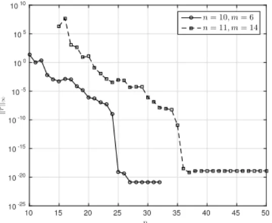
Fig. 1. The maximum absolute value of the residual for differentiating a spherical harmonic, with the maximum taken over the firstn+m spherical harmonics. In this figure, the weights are computed using variable precision arithmetic and ε = 10−10. The leveling off of the residual at O(10−20)can be attributed to the choice ofε.
4.3. Choosing the candidate stencil nodes. Increasing the size p of the candidate stencil nodes in the iterated differentiation improves accuracy of the ap-proximations to BT and C described in the previous section, but also increases the computational cost and worsens the conditioning of the linear system in (19). The-oretically, the smallest possible candidate stencil would simply include every stencil node used in the RBF-HFD formula (11). However, this choice will not lead to ac-curate weights. Numerical experiments indicate that the candidate stencil should contain at leastn+mnodes in order to obtain stable and accurate weights.
In the flat basis limit, as the shape parameter goes to zero, RBF interpolants re-produce certain polynomial interpolants in many cases [11]. Wright and Fornberg [43] provided evidence that the weights obtained from Hermite RBF interpolants in this limit are identical to classical compact weights that are exact for polynomials. For the sphere, it is natural to suppose that the Hermite weights would become exact for the spherical harmonics. This is indeed the case, if the neighborhood size is sufficiently large, which is demonstrated in Figure 1. Let the residual for an example stencil on the sphere be denoted
r= n X i=1 wiY(xi) + m X j=1 ˜ wj(∆MY) x=˜x j −(∆MY) x=x 1, (24)
where Y is a spherical harmonic. Shown in the plot in Figure 1 is the maximum absolute value of the residual, where the maximum is taken over the first n+m
spherical harmonics. Forpn+m, the weights incur errors of very large magnitude, but the error decreases rapidly aspincreases. From this plot, we posit that pmust consist of at least as many nodes as the number of spherical harmonics of one degree higher than the degree we wish the weights to be exact for. For instance, if we have
n+m = 16 and we wish the weights to be exact for all spherical harmonics up to third degree (of which there are 16), thenpmust at least be 25.
Whether the arguments above hold for other surfaces is uncertain, as this depends on the polynomial space spanned by the RBF basis in the limit as ε goes to zero. Additionally, it may not be of particular interest to explore the flat basis limit in practice, as such exploration requires multiple precision arithmetic or a stable method,
such as RBF-GA [30, 20] or RBF-QR [21, 18], for computing the weights. The choice ofpshould rather be determined by accuracy and stability concerns.
4.4. Greedy algorithm for stencil selection. If the node set is near uniform, experiments have shown that a nearest neighbor approach to stencil selection is usually sound. However, compact stencils can provide additional properties if the stencil nodes are chosen wisely. A simple greedy algorithm, similar to the one in [43], is used for this purpose. For small stencils (n, m≤10), that provide up to fourth-order convergence, we enforce that all weights in ˜LΞ are positive, that ˜LΞ is diagonally dominant, and
that all off-diagonal elements inLΞ are positive. By consistency, any row sum ofLΞ
is zero and thus the diagonal elements are negative. This property ofLΞ, along with
the diagonal dominance of ˜LΞ, provides the stability properties outlined in section 6,
while imposing positivity of the ˜LΞweights ensures that the compact weights mimic
their lattice-based counterparts. For larger stencils, such weights cannot be found, and we must give up the last property.
The greedy algorithm proceeds in the following way:
1. For each node ξk, determine the p−1 nearest neighbors to form Sk and
compute all matrices necessary to form the approximation to the entries of
AH and the right-hand side in the system (12) as described in section 4.1.
2. Compute all combinations of choosingn−1 nodes fromSk and sort them by
average distance toξk. Let{J(i)}imax
i=1 denote the set of index sets obtained.
3. Repeat step 2 withn−1 replaced bymand denote this set{J˜(j)}jmax
j=1.
4. Leti =j = 1. Until stencils with suitable weights have been found, repeat the following two steps:
5. Compute w and ˜w from the approximation (12) using the stencilsJ(i) and ˜
J(j).
6. If the weights satisfy the conditions, or i = imax and j = jmax, go to step
1 and continue with k = k+ 1. Else if j = jmax, or if j = 1 and w is not
diagonally dominant, increasei and letj= 1. Else increase j.
The rationale behind the second condition in step 6 is that, if w is not diagonally dominant, numerical experiments have shown that replacing the implicit stencil is unlikely to work. For near-uniform nodes and suitable values for the stencil and neighborhood sizes, the conditions are met for i= j = 1 for a majority of stencils, which corresponds to the nearest neighbor approach. The algorithm rarely requires more than ten iterations in steps 5 and 6.
5. Using RBF-HFD weights with the method-of-lines. In sections 7.1 and 7.2, we use the RBF-HFD discrete approximation to the surface Laplacian in the method of lines (MOL) to simulate diffusion and reaction-diffusion equations on surfaces. We briefly review this technique for the former equation, as its generalization to the latter follows naturally.
The diffusion of a scalar quantityuon a surface with a (nonlinear) forcing term is given as
∂u
∂t =δ∆Mu+f(t, u),
(25)
whereδ >0 is the diffusion coefficient,f(t, u) is the forcing term, and an initial value ofuat timet= 0 is given.
Our RBF-HFD method for (25) takes the form
d dtuΞ=δ
˜
L−Ξ1LΞuΞ+f(t, uΞ),
where ˜L−Ξ1LΞ is an RBF-HFD discretization of ∆M over the nodes in Ξ, as described
above. This is a system ofN coupled ODEs and, provided it is stable (see section 6), can be advanced in time with a suitably chosen time-integration method. In contrast to an explicit RBF-FD discretization, where ˜LΞ is the identity matrix, both explicit
and implicit time discretizations will require solving a sparse linear system. The diffusion term is typically treated implicitly in order to allow larger time steps, and we have chosen to use a semi-implicit BDF3 method [2], given by
11 6 I−δ∆t ˜ L−Ξ1LΞ unX+1= 3unX−3 2u n−1 X + 1 3u n−2 X (27) + ∆t 3f(tn, uXn)−3f(tn−1, unX−1) +f(tn−2, unX−2) ,
where the superscript denotes time level. Ifδ and ∆t are constant in time, we may multiply by ˜LΞto obtain the system
(28) 11 6 ˜ LΞ−δ∆tLΞ | {z } RΞ unX+1= ˜LΞ{r.h.s. of (27)}.
The matrix RΞ is sparse and well-conditioned, and may be factorized if a sufficient
amount of memory is available. Another option is to use a Krylov solver with a suitable preconditioner, for instance an ILU decomposition. The latter might be preferable if the time step is adaptive, since the zero-fill ILU preconditioner is cheap to compute, at least compared to a full LU factorization. The performance of this approach is discussed in section 7.
6. Stability and Gershgorin sets. One important reason to favor high-order compact stencils over their explicit counterparts is eigenvalue stability. In the clas-sical setting, where stencils are symmetric, the structure of the obtained generalized eigenvalue problem ensures stability when using any A-stable time stepping scheme. Consider (25) withf ≡0 and the corresponding compact semidiscretization
(29) d
dtuΞ= ˜L
−1 Ξ LΞuΞ.
We wish to prove that any eigenvalue of ˜L−Ξ1LΞ lies in the left half-plane, which is
a necessary condition for stability. In the following, we will consider the equivalent problem of showing that all eigenvalues of the generalized eigenvalue system
(30) Ax=λBx,
whereA=−LΞ andB= ˜LΞ lie in the right half-plane.
A common way to prove stability is to use the Gershgorin circle theorem. For instance, if A has zero row sum and positive diagonal and nonpositive off-diagonal elements, then any eigenvalue ofAmust have a nonnegative real part. We will assume thatAhas these properties, and thatB is a strictly diagonally dominant matrix with positive diagonal elements. If A and B were Hermitian, these properties would be sufficient for the eigenvalues of the generalized eigenvalue problem to have nonnegative real parts. The situation is somewhat more complicated in the nonsymmetric case.
Stewart[41] extended the Gershgorin circle theorem to generalized eigenvalues, and proved that any eigenvalue must lie in S
iΓi, where Γi is given by z ∈ C such
(31) |zbii−aii| ≤ X
j6=i
|zbij−aij|,
where aij and bij denote the elements of A and B, respectively. In contrast to the
regular Gershgorin theorem, it is quite difficult to determine the values ofzthat fulfill this inequality. By cleverly applying the triangle inequality, Kosti´c and co-workers [28] provided an approximate Gershgorin set that can be easily computed. Letri(A)
denote the absolute sum of theith row of A with the diagonal element zeroed out. Theith approximate Gershgorin set ˆΓi is given byz∈Csuch that
|zbii−aii| ≤ |z|ri(B) +ri(A).
By dividing bybii, which is positive by assumption, we obtain
(32) |z−aii bii | ≤ |z|ri(B) bii +ri(A) bii . We will letα=aii bii andβ= ri(B)
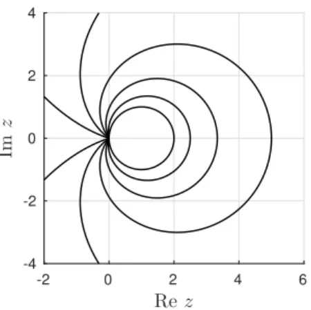
bii , and note that we haveri(A) =aii from the matrix properties we assumed. Note also thatβ <1 sinceB is strictly diagonally dominant. Approximate Gershgorin sets forα= 1 and various β are shown in Figure 2. In particular, note that none of the sets contain any part of the negative real axis. For small values ofβ, the only part of the negative real half-plane that is included in the approximate Gershgorin set is a narrow segment along the imaginary axis. In the special case whereB has nonnegative elements, it is typically possible to find stencils that provideβ <0.5, which makes the unstable part of the Gershgorin set practically insignificant.
In practice, the exact Gershgorin sets turn out to be much smaller than the approximate ones for the discretizations considered here. Examples are shown in Figure 3, where fourth-order and sixth-order approximations of the Laplace–Beltrami operator on the sphere are considered. Note that the regions shown are not the (approximate) Gershgorin set, but rather theith (approximate) Gershgorin set, where
i is chosen as the row that gives the largest extent in the left half-plane. For the fourth-order method, the Gershgorin set shown is essentially completely contained in the right half-plane.
Rez -2 0 2 4 6 I m z -4 -2 0 2 4
Fig. 2.Approximate Gershgorin sets forα= 1and various values ofβ. The circle corresponds to β = 0, and additional curves are given byβ = 0.2, 0.4, 0.6, 0.8, and 0.95, starting from the innermost to the outermost curve.
Rez -200 0 200 400 600 800 I m z -500 -400 -300 -200 -100 0 100 200 300 400 500 -40 0 40 -50 0 50
(a) Fourth-order method.
-500 0 500 1000 1500 Rez -1000 -800 -600 -400 -200 0 200 400 600 800 1000 I m z -100 0 100 -200 0 200 (b) Sixth-order method.
Fig. 3.Generalized eigenvalues of(A, B)and corresponding Gershgorin sets. Theith approx-imate Gershgorin set is outlined by a dashed line, and the respective exact one is given by a solid line, where the indexiis chosen to give the largest extent in the left half-plane of each individual set. The inset shows a magnification about the origin.
Table 1
The manifolds in the experiments are given by{x, y, z}satisfyingF(x, y, z) = 0. For the Red Blood Cell, the parameters arec0=0.a81, c2=7.a83, c4=−4a.39, andr0=3.a91 witha= 3.39. The parameters for Dupin’s Cyclide arec1= 2, c2= 1.9, c3=
√ 0.39, andc4= 1. Surface F(x, y, z) Sphere x2+y2+z2−1 Torus (1−px2+y2)2+z2−1 9
Red Blood Cell
1−x2+y2 r2 0 c0+c2 x2+y2 r2 0 +c4 x2+y2 r2 0 2!2 −4z2 Dupin’s Cyclide (x2+y2+z2−c2 4+c22)2−4(c1x+c3c4)2−4c22y2 “Tooth” x8+y8+z8−(x2+y2+z2)
7. Numerical results. The numerical experiments in this section were per-formed in MATLAB, using node sets generated by DistMesh [35, 34], unless other-wise noted. All timing experiments were run on a desktop computer equipped with an IntelR CoreTM2 Quad Q9550 processor at 2.83 GHz and 4 GB of RAM and we did
not make explicit use of parallelization inMATLAB. For a mathematical description of the manifolds, see Table 1. Example node sets are presented in Figure 4.
7.1. Parameter studies. To verify the convergence rate and facilitate compar-isons between explicit and implicit finite difference methods, we use the forced heat equation with a known analytic solution, given by Eq. (25) withδ= 1. We restrict our attention to the surface of the sphere and the torus, in order to be able to manufacture exact solutions.
As in [38], we take the exact solution for the sphere to be
(33) u(t,x) =e−5t
23
X
k=1
Fig. 4.Example node sets for the red blood cell model, Dupin’s cyclide, and the “tooth” model.
wherex∈S2 andyk,k= 1, . . . ,23, are randomly placed points onS
2. For the torus,
we also use the exact solution from [38]:
(34) u(t, λ, ϕ) =e−5t 30
X
k=1
e−20(1−cos(λ−λk))−94(1−cos(ϕ−ϕk)).
Here the solution is stated in the parametric variables (λ, ϕ)∈[−π, π]2 for the torus,
and (λk, ϕk), k = 1, . . . ,30, are taken as randomly chosen values in [−π, π]2. The
exact parameterization of the torus we use is
x= 1 + 1 3cos(ϕ) cos(λ), y= 1 + 1 3cos(ϕ) sin(λ), z= 1 3sin(ϕ). The forcing terms for the diffusion equations on the two surfaces are computed from these exact solutions. Unless otherwise noted, the diffusion equations for both surfaces are simulated for 0 ≤ t ≤ 0.2 and the time step is chosen such that spatial errors dominate. All time integrations are done using BDF3 and the forcing function is evaluated implicitly. We restrict the presentation to the relative `∞-norm of the
error as the observed convergence rates were the same for the`1-,`2-, and`∞-norms.
Finally, we let hdenote the “spacing” of the nodes in Ξ, and compute this as the average distance to the nearest neighbor.
Shape parameter. Two strategies for the scaling of the shape parameter are com-monly used: inversely proportional to the node distance h, or fixed. The former choice keeps the condition number of the regular interpolation matrix, here denoted
κ(AR), constant, but introduces a stationary interpolation error that does not
de-crease to zero in the limit ashgoes to zero. A fixedεgives convergence for allh, but the linear systems for computing the weights become ill-conditioned for smallh, and convergence is lost due to round-off errors. There are workarounds for both of these problems. In the stationary interpolation case, it is possible to recover high-order convergence by adding suitable polynomial terms to the interpolant [14, 3]. On a sur-face, however, the polynomials may themselves introduce ill-conditioning, especially if it is an algebraic surface as polynomial unisolvency becomes an issue.
If ε is kept fixed, there are currently two options to circumvent the problem of ill-conditioning: stable algorithms or variable-precision arithmetic. The algorithms of the former category, such as RBF-GA, RBF-QR, and RBF-CP[20, 18, 22], are unfor-tunately not easily adaptable to Hermite interpolation in the form introduced here. Instead, we adopt quad-precision arithmetic, for instance using the Advanpix toolbox
[1], which allows accurate determination of the weights for values ofhcorresponding to millions of nodes on the surfaces considered. Note that quad precision is only needed for the computation of the weights, after which the results can be truncated back to double precision and the simulations run without issues. Also note that com-puting the weights is an embarrassingly parallel task, and one that is only performed once for a given simulation. Optimization ofεis beyond the scope of this study, and the value is chosen such that weights can be computed in double precision for small to moderate node sets (N .50,000), after which we switch to quad precision.
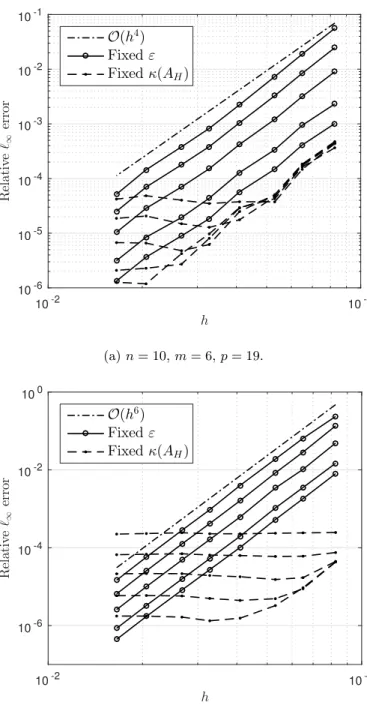
Results for the forced heat equation of the sphere illustrating the effects of the two shape parameter strategies are presented in Figures 5(a) and 5(b), in which the errors as a function ofhare shown for a fourth-order and a sixth-order approximation, respectively. In the fourth-order case, both strategies for selecting the shape param-eter converge with the same rate for a large range of values of h, but keeping the condition number fixed eventually results in a stationary error ashdecreases. For the sixth-order stencil, the resulting order is slightly lower in the fixed condition number setting, and convergence is achieved only in a small range of values ofh. Note that the mean condition number of the Hermite interpolation matrix,AH, was kept fixed
in these experiments. Similar results for the torus were observed and have thus been omitted.
Stencil sizes. The choicem=n−1 and letting the index setsIandJcoincide (bar the evaluation node) provides ideal sparsity of the matrixRΞ in Eq. (28). However,
as the approximation order is increased, it gradually becomes more difficult to find weightswthat satisfy the diagonal dominance criterion. On near-uniform nodes, it is typically possible to find stable weights fornup to 12. The stencil selection algorithm will also influence the sparsity of the matrices, and certain combinations ofnandm
are more likely to produce stable weights (e.g., by symmetry). Another consideration is the formal approximation order of the stencil, which we are not able to derive, and so instead determine it experimentally. The order appears to be primarily determined by the number of degrees of freedom of the Hermite system, i.e.,n+m.
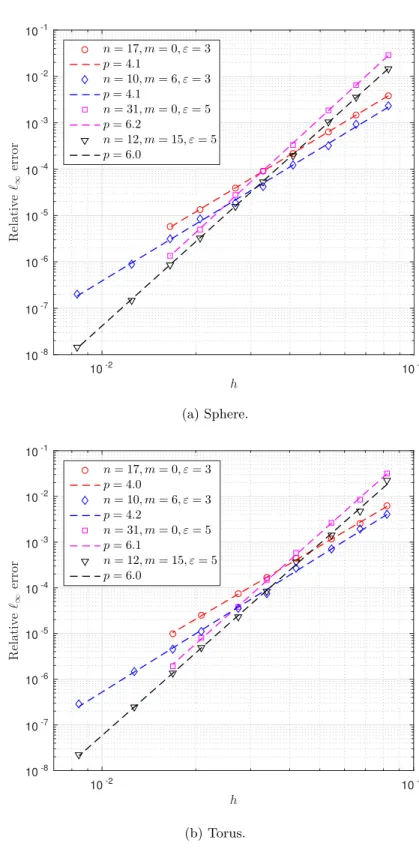
Figures 6(a) and 6(b) show the error as a function ofhfor the forced heat equation on the sphere and on the torus, respectively, with different values ofmandn. In these figures, the shape parameter is kept fixed at ε= 3 for the smaller stencil sizes and
ε = 5 for the larger ones. With these choices, quad-precision arithmetic is only required for computing the weights for the two largest node sets, which range in size fromN ≈1000 toN ≈200,000. We summarize the observations from this experiment regarding observed order of convergence and stencil sizes in Table 2.
Performance comparison. In addition to the stability properties discussed in sec-tion 6, compact stencils provide better sparsity for the same approximasec-tion order. This should lead to a smaller memory footprint and fewer floating-point operations for solving the system in Eq. (28). In this paper, we use BiCGSTAB with zero-fill ILU preconditioner for solving the linear system. Table 3 shows the number of nonzero elements in RΞ and the CPU time for a simulation for some combinations of N, n,
and m. Also presented in this table is the average number of Krylov iterations per time step. It is interesting to note from this table that, in terms of CPU time, the smaller implicit stencil barely outperforms the explicit stencil of the same order. This can be attributed to the larger number of iterations needed for the Krylov solver to converge. Increasing the stencil size to n= 12 and m = 15 reduces the number of iterations needed, plausibly due to the larger number of nonzeros in the incomplete LU factorization. This results in a CPU time that is comparable to that of the smaller implicit stencil. In this comparison, the fourth-order explicit stencil (n= 17, m= 0)
10-2 10-1 h 10-6 10-5 10-4 10-3 10-2 10-1 R e la t iv e ℓ∞ e r r o r O(h4) Fixedε Fixedκ(AH) (a)n= 10,m= 6,p= 19. 10-2 10-1 h 10-6 10-4 10-2 100 R e la t iv e ℓ∞ e r r o r O(h6 ) Fixedε Fixedκ(AH) (b)n= 12,m= 15,p= 32.
Fig. 5. The error as a function of hfor the forced heat equation on the sphere for different strategies of shape parameter selection. Solid lines correspond to fixed shape parameter, and dashed lines correspond to fixed condition number. The dash-dot line show slopes for convergence rateO(hp)
with p= 4,6. In(a) the values ofεare{6,5,4,3,2.5} from top to bottom, and in(b) the values are{8,7,6,5,4.5}, again from top to bottom. The values ofκ(AH)are{1010,1011,1012,1013,1014}
10-2 10-1 h 10-8 10-7 10-6 10-5 10-4 10-3 10-2 10-1 R e la t iv e ℓ∞ e r r o r n= 17, m= 0, ε= 3 p= 4.1 n= 10, m= 6, ε= 3 p= 4.1 n= 31, m= 0, ε= 5 p= 6.2 n= 12, m= 15, ε= 5 p= 6.0 (a) Sphere. 10-2 10-1 h 10-8 10-7 10-6 10-5 10-4 10-3 10-2 10-1 R e la t iv e ℓ∞ e r r o r n= 17, m= 0, ε= 3 p= 4.0 n= 10, m= 6, ε= 3 p= 4.2 n= 31, m= 0, ε= 5 p= 6.1 n= 12, m= 15, ε= 5 p= 6.0 (b) Torus.
Fig. 6. The error as a function ofhfor the forced heat equation with different stencil sizes. The dashed lines show slopes for convergence rateO(hp), fitted from the data points.
Table 2
Recommended stencil and neighborhood sizes for different approximation orders. The order was determined from numerical experiments on the sphere and the torus shown in Figure6.
n m p Observed order 10 6 19 4 12 15 32 6 17 0 17 4 31 0 31 6 Table 3
The table shows the number of nonzeros of the matrixRΞ, the average iteration count for the Krylov solver, and the CPU time for200time steps with∆t= 10−3 for some choices ofn,m, and
h. The surface in this experiment is the sphere, and the tolerance for the Krylov solver is10−12.
n m h N # of nonzeros Avg. iter. CPU time (s) 10 6 0.1 1806 18064 2 0.37 0.05 7446 74462 3 1.5 0.025 30054 300548 5.5 11 12 15 0.1 1806 28925 2 0.41 0.05 7446 119136 2.5 1.7 0.025 30054 480864 4 10 17 0 0.1 1806 30702 2 0.39 0.05 7446 126582 2.5 1.6 0.025 30054 510918 4 10 31 0 0.1 1806 55986 1.5 0.40 0.05 7446 230826 2 2.4 0.025 30054 931674 4 18 10-2 10-1 h 10-1 100 101 102 103 R u n -tim e [s] n= 10, m= 6 n= 12, m= 15 O(h−3)
Fig. 7. The run-time for a simulation of the forced heat equation on the sphere as a function ofh, using∆t= 10−2·h. The simulation was run fromt= 0tot= 0.2.
is on par with the sixth-order implicit stencil both in terms of memory requirements and computational cost. Note that the time step chosen, ∆t= 10−3, is rather small
(which is needed for spatial errors to dominate). Increasing the time step to ∆t= 0.1 increases the number of Krylov iterations per time step roughly by a factor of 6.
In most applications, ∆t would be chosen proportional to h in order to reduce both spatial and temporal errors as the node set is refined. Figure 7 shows the CPU
time as a function of h with ∆t = 10−2·h. For the near-uniform node sets used
throughout this paper,N ∝1/√h, and thus the CPU time scales asO(N3/2). 7.2. Applications. We now present applications of the new compact scheme to solving reaction-diffusion equations on different surfaces. As in [38], we present results of simulations both on surfaces defined implicitly by algebraic expressions (see Table 1) and on more general point cloud surfaces. On the former, we simulate the same two-species Turing system used in [38], given by
∂u ∂t =αu(1−τ1v 2 ) +v(1−τ2u) +δu∆Mu, (35) ∂v ∂t =βv 1 + ατ1 β uv +u(γ+τ2v) +δv∆Mv. (36)
A visualization of the solutions of this equation on the various surfaces with the parameters selected from Table 4 are shown in Figure 8.
Table 4
The table shows the values of the parameters of (35)and(36)used in the numerical experiments shown in Figure8. We setδu= 0.516δvfor the red blood cell and tooth models, and useδu= 5.16δv
for Dupin’s cyclide.
Pattern δv α β γ τ1 τ2 Final time
Spots 4.5×10⁻³ 0.899 −0.91 −0.899 0.02 0.2 200
Stripes 2.1×10⁻³ 0.899 −0.91 −0.899 3.5 0 4000
Fig. 8. Quasi-steady Turing spots and stripe patterns resulting from solving (35)and (36)
on the red blood cell model, Dupin’s cyclide, and the “tooth” model using the fourth-order compact scheme. In all plots, light shading indicates high concentrations and dark shading indicates low concentrations (the electronic version is full-color).
Fig. 9. Fitzhugh–Nagumo spiral wave patterns resulting from solving (37)and (38)on the bumpy sphere and bunny models using the fourth-order compact scheme. In all plots, light shading indicates high concentrations and dark shading indicates low concentrations (the electronic version is full-color).
On the more general point cloud surfaces, we simulate the Fitzhugh–Nagumo-type model used in [26]: ∂u ∂t =δu∆Mu+ 1 αu(1−u) u−v+b a , (37) ∂v ∂t =δv∆Mv+u−v. (38)
For both the bumpy sphere2 and bunny3 models, we set a = 0.75, b = α = 0.02, δv = 0, and δu = 1.5(250π)2. With these parameters, the model generates dynamic
spiral wave solutions. Snapshots of these solutions computed with the RBF-HFD method for the two surfaces are shown in Figure 9. We note that the normal vectors on these point cloud models can be generated by any appropriate method. In this work, the node sets and normal vectors were created using MeshLab [8], utilizing the Poisson surface reconstruction algorithm with some additional smoothing and the Poisson disk sampling method.
7.3. Curvature, node spacing, and the stencil selection algorithm. In a few of our experiments, the greedy algorithm failed to find suitable stencils for some
2Available from the Aim@Shape Shape Repository (http://visionair.ge.imati.cnr.it/).
3Available from the Stanford Computer Graphics Laboratory (http://graphics.stanford.edu/
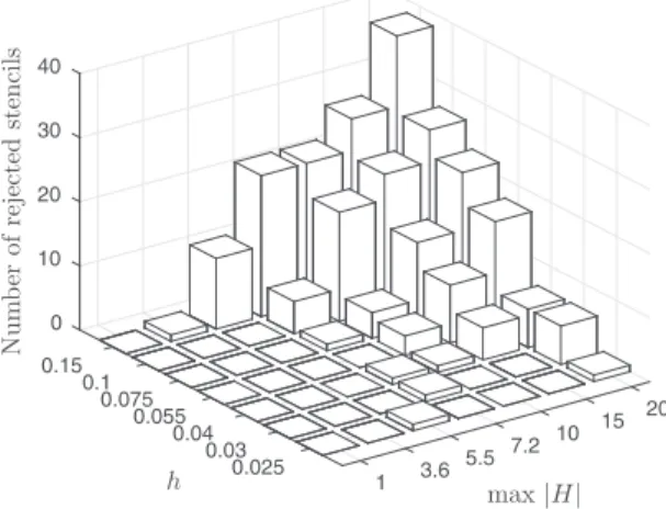
Fig. 10. The number of rejected stencils as a function ofhand the mean curvatureH.
node points. A common characteristic of these nodes was that they were located in areas of large curvature, e.g., around the ears of the bunny. To illustrate this curvature effect more clearly on the failure of the stencil selection algorithm, we carried out an experiment generating the surface Laplacian on prolate spheroids of varying curvatures and determining how the number of rejected stencils changed with curvature. The results are plotted in Figure 10 in terms of the number of rejected stencils, i.e., stencils where the stability constraints could not be met, as a function of both the node distance h and the maximum mean curvature H. Note that imax
and jmax in the greedy algorithm were set to 5 in this experiment so that only a
small number of stencils were attempted for each node, to emphasize the effect of the curvature. This experiment indicates that decreasing the node spacing alleviates the issue. In our experiments on the bunny, we found that simply using nearest neighbor stencils for cases where no suitable stencil could be found still led to temporal stability, and we therefore recommend this approach. Two other potential remedies are increasing εfor the nodes where no suitable stencils can be found, and refining the node set locally in these areas. The former has previously been noted to improve stability (see, e.g., [16]), but larger values of ε also tend to reduce the accuracy. A full exploration of these latter two approaches is beyond the scope of this work.
8. Discussion. The compact RBF-HFD scheme improves on previous RBF-FD schemes for diffusion on surfaces both in terms of efficiency and stability. The pro-posed greedy stencil selection algorithm ensures eigenvalue stability on surfaces with-out large (or rapid) changes in curvature. In numerical experiments of the forced diffusion equation on the sphere and the torus, the new scheme provided accuracy similar to the previous noncompact RBF-FD method, but with a smaller memory footprint and higher accuracy. The linear systems generated from the semi-implicit BDF3 time discretization were also shown to be efficiently solvable using BiCGStab with a standard zero-fill ILU preconditioner. In addition to illustrating the good stability, accuracy, and efficiency properties of the scheme, we showed how it can be easily adaptable to reaction-diffusion equations on both implicitly defined surfaces and surfaces defined by a point cloud. The method can be naturally generalized to a smooth orientable surface that is discretized with a set of roughly uniform nodes and with approximations to the normal to the surface at each of the nodes.
While stencil sizes generating fourth- and sixth-order convergence in numerical ex-periments on the sphere and the torus are provided, no investigation of the theoretical convergence rates have been given. This is clearly an avenue of future investigation. Another future topic of research is the influence of the curvature and the shape pa-rameter on the computed RBF-HFD weights. Experiments suggest that large local curvature makes it impossible to find weights that satisfy the conditions that ensure eigenvalue stability, although no issues with temporal integration were encountered when this stability was not insured. Refining the node sets in areas of high curvature or increasing the shape parameters used in the stencils in these areas may provide a simple way to alleviate the problem. An extensive investigation of the relationship between curvature, nodal distance, and stability will the topic of a future study.
Finally, we note that an extension to convection-diffusion problems would allow the method to be used in various applications, e.g., chemical transport on thin mem-branes and shells, biomechanical modeling of cells. This is currently being pursued by the first author.
REFERENCES
[1] Advanpix Multiprecision Computing Toolbox for MATLAB, http://www.advanpix.com/, ac-cessed 2016-06-09.
[2] U. M. Ascher, S. J. Ruuth, and B. T. R. Wetton, Implicit-explicit methods for time-dependent PDEs, SIAM J. Numer. Anal, 32 (1997), pp. 797–823.
[3] V. Bayona, N. Flyer, B. Fornberg, and G. A. Barnett,On the role of polynomials in RBF-FD approximations: II. Numerical solution of elliptic PDEs, J. Comput. Phys., 332 (2017), pp. 257–273.
[4] V. Bayona, M. Moscoso, M. Carretero, and M. Kindelan,RBF-FD formulas and con-vergence properties, J. Comput. Phys., 229 (2010), pp. 8281–8295.
[5] R. L. Bishop and S. I. Goldberg,Tensor Analysis on Manifolds, Macmillan, New York, 1968. [6] T. Cecil, J. Qian, and S. Osher,Numerical methods for high dimensional Hamilton–Jacobi
equations using radial basis functions, J. Comput. Phys., 196 (2004), pp. 327–347. [7] G. Chandhini and Y. Sanyasiraju,Local RBF-FD solutions for steady convection–diffusion
problems, Int. J. Numer. Meth., 72 (2007), pp. 352–378.
[8] P. Cignoni, M. Corsini, and G. Ranzuglia,MESHLAB: An open-source3D mesh processing system, ERCIM News, (2008), pp. 45–46.
[9] L. Collatz, The Numerical Treatment of Differential Equations, 3rd ed., Springer, Berlin, 1966.
[10] O. Davydov and D. T. Oanh,Adaptive meshless centres and RBF stencils for Poisson equa-tion, J. Comput. Phys., 230 (2011), pp. 287–304.
[11] T. A. Driscoll and B. Fornberg,Interpolation in the limit of increasingly flat radial basis functions, Comput. Math. Appl., 43 (2002), pp. 413–422.
[12] G. E. Fasshauer,Meshfree Approximation Methods with MATLAB, Interdisciplinary Mathe-matical Sciences 6, World Scientific, Singapore, 2007.
[13] G. E. Fasshauer and M. J. McCourt,Stable evaluation of Gaussian radial basis function interpolants, SIAM J. Sci. Comput., 34 (2012), pp. A737–A762.
[14] N. Flyer, B. Fornberg, V. Bayona, and G. A. Barnett,On the role of polynomials in RBF-FD approximations I. Interpolation and accuracy, J. Comput. Phys., 321 (2016), pp. 21–38.
[15] N. Flyer, E. Lehto, S. Blaise, G. B. Wright, and A. St-Cyr,A guide to RBF-generated finite differences for nonlinear transport: Shallow water simulations on a sphere, J. Com-put. Phys., 231 (2012), pp. 4078–4095.
[16] N. Flyer and G. B. Wright,A radial basis function method for the shallow water equations on a sphere, Proc. R. Soc. A, 465 (2009), pp. 1949–1976.
[17] B. Fornberg and N. Flyer,A Primer on Radial Basis Functions with Applications to the Geosciences, SIAM, Philadelphia, 2014.
[18] B. Fornberg, E. Larsson, and N. Flyer, Stable computations with Gaussian radial basis functions, SIAM J. Sci. Comput., 33 (2011), pp. 869–892.
[19] B. Fornberg and E. Lehto, Stabilization of RBF-generated finite difference methods for convective PDEs, J. Comput. Phys., 230 (2011), pp. 2270–2285.
[20] B. Fornberg, E. Lehto, and C. Powell, Stable calculation of Gaussian-based RBF-FD stencils, Comput. Math. Appl., 65 (2013), pp. 627–637.
[21] B. Fornberg and C. Piret,A stable algorithm for flat radial basis functions on a sphere, SIAM J. Sci. Comput., 30 (2007), pp. 60–80.
[22] B. Fornberg and G. Wright,Stable computation of multiquadric interpolants for all values of the shape parameter, Comput. Math. Appl., 48 (2004), pp. 853–867.
[23] B. Fornberg and J. Zuev,The Runge phenomenon and spatially variable shape parameters in RBF interpolation, Comput. Math. Appl., 54 (2007), pp. 379–398.
[24] E. Fuselier and G. Wright,Scattered data interpolation on embedded submanifolds with restricted positive definite kernels: Sobolev error estimates, SIAM J. Numer. Anal., 50 (2012), pp. 1753–1776.
[25] E. Fuselier and G. B. Wright, Order-preserving derivative approximation with periodic radial basis functions, SIAM J. Numer. Anal., 41 (2015), pp. 23–53.
[26] E. J. Fuselier and G. B. Wright,A high-order kernel method for diffusion and reaction-diffusion equations on surfaces, J. Sci. Comput., (2013), pp. 1–31.
[27] Q. T. L. Gia,Approximation of parabolic pdes on spheres using spherical basis functions, Adv. Comput. Math., 22 (2005), pp. 377–397.
[28] V. Kosti´c, R. S. Varga, and L. Cvetkovi´c,Localization of generalized eigenvalues by Carte-sian ovals, Numer. Linear Algebra Appl., 19 (2012), pp. 728–741.
[29] E. Larsson and B. Fornberg,Theoretical and computational aspects of multivariate inter-polation with increasingly flat radial basis functions, Comput. Math. Appl., 49 (2005), pp. 103–130.
[30] E. Larsson, E. Lehto, A. Heryudono, and B. Fornberg,Stable computation of differentia-tion matrices and scattered node stencils based on Gaussian radial basis funcdifferentia-tions, SIAM J. Sci. Comput., 35 (2013), pp. A2096–A2119.
[31] S. K. Lele,Compact finite difference schemes with spectral-like resolution, J. Comput. Phys., 103 (1992), pp. 16–42.
[32] C. Macdonald and S. Ruuth,The implicit closest point method for the numerical solution of partial differential equations on surfaces, SIAM J. Sci. Comput., 31 (2010), pp. 4330–4350. [33] F. Narcowich and J. Ward,Generalized hermite interpolation via matrix-valued conditionally
positive definite functions, Math. Comput., 63 (1994), pp. 661–688.
[34] P.-O. Persson,DistMesh – a simple mesh generator in MATLAB. http://persson.berkeley. edu/distmesh/, accessed 2016-06-09.
[35] P.-O. Persson and G. Strang,A simple mesh generator in MATLAB, SIAM Rev., 46 (2004), pp. 329–345.
[36] C. Piret,The orthogonal gradients method: A radial basis functions method for solving partial differential equations on arbitrary surfaces, J. Comput. Phys., 231 (2012), pp. 4662–4675. [37] R. Schaback,Multivariate interpolation by polynomials and radial basis functions, Constr.
Approx., 21 (2005), pp. 293–317.
[38] V. Shankar, G. B. Wright, R. M. Kirby, and A. L. Fogelson, A radial basis function (RBF)-finite difference (FD) method for diffusion and reaction–diffusion equations on surfaces, J. Sci. Comput., 63 (2014), pp. 745–768.
[39] C. Shu, H. Ding, and K. S. Yeo, Local radial basis function-based differential quadrature method and its application to solve two-dimensional incompressible Navier–Stokes equa-tions, Comput. Methods Appl. Mech. Eng., 192 (2003), pp. 941–954.
[40] D. Stevens, H. Power, M. Lees, and H. Morvan,The use of PDE centers in the local RBF Hermitean method for3D convective-diffusion problems, J. Comput. Phys., 228 (2009), pp. 4606–4624.
[41] G. W. Stewart,Gershgorin theory for the generalized eigenvalue problemAx=λBx, Math. Comput., 29 (1975), pp. 600–606.
[42] G. B. Wright, N. Flyer, and D. A. Yuen,A hybrid radial basis function–pseudospectral method for thermal convection in a3-D spherical shell, Geochem. Geophys. Geosyst., 11 (2010).
[43] G. B. Wright and B. Fornberg,Scattered node compact finite difference-type formulas gen-erated from radial basis functions, J. Comput. Phys., 212 (2006), pp. 99–123.
[44] W. Zongmin,Hermite–Birkhoff interpolation of scattered data by radial basis functions, Ap-prox. Theory Appl., 8 (1992), pp. 1–10.
![[18F]-Fluorodeoxyglucose Uptake in Lymphoid Tissue Serves as a Predictor of Disease Outcome in the Nonhuman Primate Model of Monkeypox Virus Infection](data:image/gif;base64,R0lGODlhAQABAIAAAP///wAAACH5BAEAAAAALAAAAAABAAEAAAICRAEAOw==)