u n i ve r s i t y o f co pe n h ag e n
Testing and Inference in Nonlinear Cointegrating Vector Error Correction Models
Kristensen, Dennis; Rahbek, Anders
Publication date:
2010
Document version
Publisher's PDF, also known as Version of record
Citation for published version (APA):
Kristensen, D., & Rahbek, A. (2010). Testing and Inference in Nonlinear Cointegrating Vector Error Correction
Discussion Papers
Department of Economics
University of Copenhagen
Øster Farimagsgade 5, Building 26, DK-1353 Copenhagen K., Denmark
Tel.: +45 35 32 30 01 – Fax: +45 35 32 30 00
ISSN: 1601-2461 (E)
No. 10-25
Testing and Inference in Nonlinear Cointegrating
Vector Error Correction Models
Dennis Kristensen, Anders Rahbek
Testing and Inference in Nonlinear
Cointegrating Vector Error Correction Models
Dennis Kristenseny Columbia University Anders Rahbekz University of Copenhagen October, 2010 Abstract
In this paper, we consider a general class of vector error correction models which allow for asymmetric and non-linear error correction. We provide asymptotic results for (quasi-)maximum likelihood (QML) based estimators and tests. General hypothesis testing is considered, where testing for linearity is of particular interest as parameters of non-linear components vanish under the null. To solve the latter type of testing, we use the so-calledsuptests, which here requires development of new (uniform) weak convergence results. These results are potentially useful in general for analysis of non-stationary non-linear time series models. Thus the paper provides a full asymptotic theory for estimators as well as standard and non-standard test statistics. The derived asymptotic results prove to be new compared to results found elsewhere in the literature due to the impact of the estimated cointegration relations. With respect to testing, this makes implementation of testing involved, and bootstrap versions of the tests are proposed in order to facilitate their usage. The asymptotic results regarding the QML estimators extend results in Kristensen and Rahbek (2010, Journal of Econometrics) where symmetric non-linear error correction considered. A simulation study shows that the …nite sample properties of the bootstrapped tests are satisfactory with good size and power properties for reasonable sample sizes.
Both authors are a¢ liated with CREATES funded by the Danish National Research Foundation. We wish to thank participants at the 18th Annual Symposium of the Society for Nonlinear Dynamics and Econometrics, in Novara, Italy, and participants at Montreal Econometrics Seminars and Oxbridge Time Series Group Workshops, Cambridge, for helpful comments and suggestions. Also we are grateful to discussions with M. Seo, LSE, London. The Velux Foundation funded a longer research visit for Kristensen to Copenhagen University, where part of this research was conducted. Part of the research was also conducted while Kristensen visited Princeton University whose hospitality is gratefully acknowledged. Kristensen received research support from the National Science Foundation (grant no. SES-0961596).
yE-mail: [email protected] zE-mail: [email protected]
1
Introduction
We develop estimators and test statistics for a class of nonlinear vector error correction models with cointegration. Both estimators and test statistics are based on the Gaussian (quasi-)likelihood, and we propose both Lagrange Multiplier (LM) and Likelihood Ratio (LR) test statistics. Our framework allows for testing a wide range of relevant hypotheses. Of particular interest is the hypothesis of nonlinearity, where in general nuisance parameters entering the nonlinear component vanish under the null. We solve this problem by employing sup-tests as advocated in Andrews and Ploberger (1994, 1995), Davies (1987), Hansen (1996) and Hansen and Seo (2002). We derive the asymptotic distributions of both estimators and test statistics under weak restrictions. As part of the theoretical analysis, new functional central limit theorems are developed which are of independent interest in the analysis of nonlinear, non-stationary models.
Allowing for unknown cointegration relations prove to complicate the analysis and the re-sulting asymptotic distributions of both the quasi-maximum likelihood estimators (QMLE’s) and test statistics considerably. In particular, we …nd non-standard limiting distributions of both estimators and test statistics, when compared to the ones established in linear coin-tegration models and for nonlinear stationary models, including coincoin-tegration models with known long-run parameters. This is due to the fact that the limiting distributions of the es-timators of the long-run and short-run parameters are not asymptotically independent. This again spills over to the distribution of the test statistics which are in‡uenced by both the estimated long-run and short-run parameters. This happens even in the case when the null hypothesis only involves restrictions on either of the parameters. If in addition parameters vanish under the null, as is often the case in testing for linearity in the short-run dynam-ics, the limiting distributions complicate further, and the proposed sup-tests are shown to converge towards a supremum over a squared non-Gaussian process.
As such, our results show that one cannot ignore the estimation of the long-run para-meters if these are unknown. This also explains why our …ndings are di¤erent from existing results on testing in nonlinear time series models. In particular, as discussed in further detail below, previous studies investigating sup-tests in cointegration models either assume that the cointegrating relations are known, or that the additional estimation error due to unknown (super consistent) relations does not a¤ect the tests.
Hansen (1996) develops an asymptotic theory for sup-tests in a stationary setting. In this case, the limiting distributions can be written as a supremum over squared Gaussian processes. This theory is extended to threshold and smooth transition cointegration models with known cointegrating relations ( ) in Gonzalo and Pitarakis (2006) and Kilic (2009) respectively. Since is assumed known, their models and results become similar to the ones of Hansen (1996).
Our results regarding suptests for linearity are related to the ones of Caner and Hansen (2001) who test for linearity in univariate threshold autoregressions with unit roots. We …nd in the multivariate case, as they do for the univariate case, that the limiting distribution of the sup test statistic consists of two terms: A stationary component due to the short-run
parameters and a non-stationary component due to the presence of unknown long-run para-meters. On the other hand, our results di¤er from Hansen and Seo (2002) and Nedeljkovic (2008), where sup-tests of linearity in threshold and smooth transition cointegration models respectively are considered, as they (implicitly) assume that estimators of have no impact on the asymptotic behaviour of their test statistic. That is, they conclude that limiting distributions can be represented as supremums over squared Gaussian processes. Finally, we note that in a di¤erent vein some studies have proposed to test for linearity by approximating the true model using a Taylor expansion of the non-linear component (Choi and Saikkonen, 2004; Kapetanios, Shin and Snell, 2006). This removes the problem of vanishing parameters, but on the other hand introduces asymptotic biases of estimators and test statistics under the alternative, since a misspeci…ed model is being employed.
A number of other studies have developed and analyzed estimators for cointegration models with non-linear error correction. In particular, Kristensen and Rahbek (2010) derive the properties of QMLE for class of smooth nonlinear error-correction models. However, they restrict themselves to the case of symmetric error-correction while we also allow for asymmetric adjustments. Thus, our …ndings regarding the QMLE generalize and improve upon the results found in that study. Our results also complement the ones of Seo (2010) who consider estimation of threshold error correction models using kernel smoothers to handle discontinuities implied by the thresholds.
To establish our theoretical results, it proves necessary to develop a new functional cen-tral limit theorems (FCLT’s) uniformly over the unidenti…ed parameters. Such results are useful in the analysis of nonlinear models with non-stationary components, and we therefore establish uniform FCLT’s in a general framework that includes, but is not restricted to, the particular class of non-linear error correction models of this study. These results generalize the ones established in Caner and Hansen (2001, Section 2) and will be useful in the analysis of other non-linear time series models; as such, they should be of independent interest.
Due to the highly non-standard limiting distribution of estimators and test statistics, we propose to implement the estimation and testing procedures using bootstrapping based on the ideas developed in Cavaliere, Rahbek and Taylor (2010a,b). In particular, we propose to use the wild bootstrap, which should make the bootstrap tests robust to heteroskedasticity. Seo (2006,2008a) and Gonzalo and Pitarakis (2006) also consider bootstrap methods for testing in non-stationary time series models but in di¤erent settings. A simulation study investigates the …nite sample performance of the proposed bootstrap version of the sup-LR test. We …nd that the proposed testing scheme has good size and power properties and so o¤er a convenient tool for inference in nonlinear error correction models.
The remains of the paper is organized as follows: We present the model and propose estimators and test statistics of the parameters in Section 2. The auxiliary functional central limit theorems (FCLT) are derived in Section 3. These are then in turn used in Section 4 and 5 to derive the limiting distributions of estimators and test statistics respectively. A bootstrap procedure for evaluating the distribution of the test statistic is proposed in Section 6, while Section 7 presents the results of a simulation study. Section 8 concludes. All proofs and lemmas have been relegated to Appendices A-B and C-D respectively.
Throughout, the following notation will be used: We use!P and!D to denote convergence in probability and distribution respectively;C(A)andD(A)denote the space of continuous and cadlag functions with domain A; df(x;dx) denotes the di¤erential of a mapping f(x) in the directiondx; byvec(a; b), we mean vec(a)0; vec(b)0 0:For any parameter , 0 will
denote its true, data-generating value; for any matrix m n matrix A of full column rank
n m, we de…ne A =A(A0A) 1, and A? as a m (m n) matrix such that [A; A?]has full rankm and A0A?= 0.
2
Framework
2.1 Model
LetXt2Rp,t= 1; :::; T, be observations from the following error correction model (ECM),
Xt=g 0Xt 1 + 1 Xt 1+:::+ k Xt k+"t; (2.1)
where Xt=Xt Xt 1 and the error term"t satis…es
E["tjFt 1] = 0; E "t"0tjFt 1 <1; (2.2)
with Ft 1 = F(Xt 1; Xt 2; :::) denoting the information set based on past values of Xt.
The functiong( )describes the (potentially nonlinear) error correction towards the long-run equilibrium. The equilibrium of the process is characterized by the cointegration relations; namely, ther 1linear combinations 0Xt, with 2Rp r.
Without loss of generality, we specify g( ) as composed by a linear and nonlinear part:
g 0Xt 1 = 0Xt 1+ 0Xt 1; : (2.3)
In this general class of speci…cations, the deviation from the basic linear ECM is given by the r -dimensional vector function ( 0Xt 1; ) multiplied by the (p r )-dimensional
pa-rameter . The papa-rameter in the nonlinear component may contain matrices and we let
d = dim (vec( ))denote the dimension of the vectorized version of . The above speci…ca-tion is su¢ ciently general to cover most known nonlinear error correcspeci…ca-tion models found in the literature. Note that we here suppress the dependence of g( ) on the parameters, ;
and .
The form of g in eq. (2.3) embeds various smooth transition error correction models. In general, allowing forS di¤erent regimes in ( ) indexed bys= 1; :::; S;we may write,
(z; ) =
S
X
s=1
s s(z; ) with := ( 1; :::; S), (z; ) := ( 1(z; ); :::; S(z; ))0: (2.4)
Depending on the functional form of the s, this formulation allow for both symmetric and
asymmetric response functions. A key example of the …rst type is the logistic STECM in Kristensen and Rahbek (2010), where
s(z; ) := 1 + exp (z !s)0As(z !s)
1
withAspositive de…nite(r r)-dimensional matrices, while!iarer-dimensional vectors, and
r =Sr. The parameter is given by = (!; A) with!= (!1; :::; !S) and A= (A1; :::; AS).
With (z; ) chosen this way, observe that (z) = o(1) as kzk ! 1 and, hence for large deviations as measured by Zt = 0Xt, the linear component z of g(z; ) in eq. (2.3)
asymptotically dominates. Also note that the nonlinearity vanishes if indeed = 0, in which case the STECM reduces to the linear ECM with g(z; ) = z. To allow for asymmetric responses, Saikkonen (2008) studies alternative general speci…cations of : An example of Saikkonen (2008) is
s(z; ) = 1 + exp a0s(z !s) 1z; (2.6)
withas being an r dimensional vector. Depending on whether(z !i) is orthogonal to as
as kzk ! 1; s(z; ) will also asymptotically be contributing to the linear z part in the
error correction. The above class of models also contains threshold models where (z; ) contains indicator functions, see e.g. Hansen and Seo (2003) and Seo (2010). However, we will impose smoothness restrictions on (z; )when analyzing our proposed estimators and test statistics which rule out threshold models. These could potentially however be dealt with by modifying our proposed estimators, replacing indicator functions by kernel smoothers, see e.g. Seo (2010), but will not be considered here.
Regarding identi…cation, then as common in the cointegration literature is identi…ed up to a normalization and we therefore normalize conveniently using a (p (p r)) di-mensional matrix 0, such that
0= 0b; (2.7)
and bis the ((p r) r) dimensional parameter to be estimated. Thus,b0 = 0 corresponds
to the true parameter value 0. Using this, we can rewrite the model in eq. (2.1) as a
nonlinear regression model in terms of(Z0;t; Z1;t; Z2;t),
Xt=g Z0;t 1+b0Z1;t 1 + Z2;t 1+"t; (2.8)
where
Z0;t:= 00Xt2Rr; Z1;t :=Xt0 0 2Rp r; Z2;t := Xt0; :::; Xt k0 +1
0
2Rpk:
As argued in Kristensen and Rahbek (2010), the estimator of the error covariance matrix, , will be asymptotically independent of the estimators of the other parameters (appearing in the conditional mean speci…cation). We therefore collect all the conditional mean parameters in#and leave out which is treated separately. Finally, note that under the null of linearity ( = 0) the parameter vanishes. To emphasize the role played by the vanishing parameter , we introduce which contains all parameter in#except for . Furthermore, we di¤erentiate between short-run and long-run parameters and collect the former in . Thus the parameters of interest are given by:
#:= ( ; ) = (b; ; ); := ( ; ; ) = ( ; ; 1; 2; :::; k): (2.9)
2.2 Estimation
Our proposed estimators are based on the Gaussian log-likelihood. In order to write the log-likelihood function, de…ne the residuals,
"t( ; ) = Xt Z0;t 1+b0Z1;t 1 Z0;t 1+b0Z1;t 1; Z2;t 1: (2.10)
Then, given T observations, X1; X2; :::; XT, and with the initial values X0; X0; :::; X k
…xed, the log-likelihood function based on Gaussian errors takes the form,
LT( ; ; ) = T 2 logj j 1 2 T X t=1 "t( ; )0 1"t( ; ): (2.11)
We de…ne the corresponding pro…led log-likelihood LT( ; ) =LT ( ; ; ( ; ))where
( ; ) = 1 T T X t=1 "t( ; )"t( ; )0;
and #^is found as,
^
#:= (^;^) = arg max
2 ; 2 LT( ; ):
As we do not impose any distributional assumptions on the errors,#^= (^;^)and ^ = (^;^)
are referred to as quasi-maximum likelihood estimators (QMLE’s).
2.3 Hypothesis Testing
We are interested in developing inference regarding both short-run ( and ) and long-run parameters ( ;orb) in the non-linear error correction model. We consider in turn hypotheses involving short- and long-run parameters.
2.3.1 Testing Short-Run Parameters
First, consider the following general hypothesis involving the short-run parameters and (cf. eq. (2.9)),
H0 :R0vec( ; ) = 0; (2.12) whereR is a known (m d)-matrix with d=p(r+d +pk) +d and m d, and we have used the notation vec( ; ) = vec( )0; vec( )0 0 mentioned in the introduction. Some key examples that are included in the above general formulation include:
Example 1 (Linear error correction) To see if the non-linear components are relevant
in explaining the error-correction mechanism, it is of interest to test for their signif-icance. One can do so by testing that there are no nonlinearities in all variables,
R0vec( ; ) =vec( ) = 0. Alternatively, we may wish to test for presence of non-linear error-correction in individual variables. For example,R0vec( ; ) = R0vec( ) = 0 for some matrixR .
Example 2 (Symmetric response) Suppose that our nonlinear component in eq. (2.3) takes the form
(z; ) = 2 X s=1 s s(z; ); where s(z; ) := 1 + exp (z !s)0As(z !s) 1 z; s= 1;2;
such that we have 2 non-linear components in addition to the linear. It is then of interest to test for symmetric responses. That is,R0vec( ; ) =vec( 1 2) = 0.
Example 3 (Weak exogeneity) Corresponding to notion of weak exogeneity in linear
er-ror correction models with respect to , we may wish to test for no error correction (neither linear, nor non-linear) in some variables. That isR0vec( ; ) =R0
; [ ; ] = 0
for some matrixR ; .
Example 4 (# lags) To choose the number of lags included in the model, the following
hypothesis is of interest,R0vec( ; ) =vec( j) = 0, for somej2 f1; :::; kg.
UnderH0, some (if not all) parameters in may vanish. One has to check this on a
case-by-case basis. One particular case is given in Example 1 where the parameter vanishes under the null of linearity. If this is the case, we face a non-standard testing problem, which is here solved by employing so-called sup-tests. Thus, we treat the two cases ( is identi…ed or unidenti…ed under the null) separately:
First, suppose is identi…ed under H0. In order to test the null, we …rst obtain the
restricted estimator of all parameters,#= ( ; ), underH0 which we denote #~= (~;~): (~;~) = arg max
#
R0vec( ;)=0
LT ( ; ):
We then propose to test the null by either LR or LM test statistics. The LR statistic compares the log-likelihoods evaluated under the alternative and under the null and is given by
LRT = 2
h
LT(^;^) LT(~;~)
i
: (2.13)
The LM statistic on the other hand, uses the score under the alternative evaluated at the parameter estimates obtained under the null,
LMT =ST(~;~)0HT1(~;~)ST(~;~); (2.14)
where ST( ; ) and HT( ; ) are the score and Hessian matrices respectively. Here ST( ; )
and HT( ; ) are identi…ed in terms of di¤erentials as introduced in Section 2.4.
Next, in the case where is unidenti…ed under the null ofH0, …rst note that the parameter
restrictions in this case cannot involve since we are unable to test for such. So after removing potentially redundant restrictions involving , the general null in eq. (2.12) can be rewritten as
for some matrixR . The estimator of = (b; ) under the null is given by ~ = arg max
2
R0vec( )=0
LT (b; ; ):
On the other hand, under the alternative, we compute a pro…le estimator of for any given value of ,
^( ) = arg max
2 LT ( ; ):
The sup-LR test is then obtained by taking supremum of the standard LR test over , supLRT := sup 2 LRT ( ); (2.15) where LRT( ) = 2 h LT(^( ); ) LT(~; )i: (2.16) The sup-LM test is obtained in a similar manner,
supLMT := sup
2
LMT( ); (2.17)
where
LMT ( ) =ST(~( ); )0HT1(~( ); )ST(~( ); ): (2.18)
2.3.2 Testing Long-Run Parameters
Recall that is identi…ed by eq. (2.7), so consider the following hypothesis involving the long-run parameter b,
H0;b:R0bvec b0 = 0; (2.19)
where Rb is a known (m d)-matrix with d= (p r)r and m d. A key example is the
following:
Example 5 (Cointegrating vectors) Economic theory often imposes, or implies, testable
restrictions on the cointegrating relations, for example that they are known. One speci…c example (with p = 2 and r = 1) is = (1; 1)0 corresponding to the spread between the two variables being stable. In terms of b 2 R, this can be expressed as
R0bvec(b0) =b= 0.
The test statistics are computed in the same way as in the previous subsection with identi…ed . We …rst compute the restricted estimators which for ease of notation we still call ~and ~: H0;b: (~;~) = arg max # R0 bvec(b0)=0 LT ( ; ):
The corresponding LR- and LM-test are then given as:
LRb;T = 2
h
LT(^;^) LT(~;~)i; LMb;T =ST(~;~)0HT1(~;~)ST(~;~):
2.4 Score and Hessian
As is standard, the analysis of likelihood-based estimators and test statistics will focus on the score and Hessian of the log-likelihood. For ease of notation, we here choose to de…ne them in terms of …rst and second order di¤erentials of the log-likelihood since parameters enter in the form of matrices; see Magnus and Neudecker (1988) for an introduction to the concept of di¤erentials and their use in econometrics. We apply standard notation and let
dLT ( ; ;d ; d ) denote the …rst-order di¤erential of LT( ; ) w.r.t. ( ; ) in the direction of d and d respectively. The vector score ST( ; ) = @LT( ; )=@vec( ; ) can then be
identi…ed from the di¤erential through the following identity:
dLT ( ; ;d ; d ) =ST( ; )0vec(d ; d ):
Similarly, withd2L
T ( ; ;d ; d ;d ; d ) denoting the second order di¤erential, the Hessian
HT( ; ) =@LT ( ; )=(@vec( ; )@vec( ; )0)is given through the following identity:
d2LT( ; ;d ; d ;d ; d ) =vec(d ; d )0HT( ; )vec(d ; d ):
To derive expressions of the …rst and second order di¤erentials of the log-likelihood, some further notation is needed: First, we introduce the di¤erentials of (z; )2Rr with respect toz2Rr and vec( )2Rd in terms of its partial derivatives,
d (z; ;dz) =@z (z; )dz, @z (z; ) = (@ i=@zj)i;j 2Rr r; (2.20)
d (z; ;d ) =@ (z; )vec(d ); @ (z; )2Rr d :
Furthermore, de…ne the processesut( )2Rp(r+r+pk),vt( )2Rr and wt( )2Rr by
ut( ) := u ;t( )0; u ;t( )0; u;t( )0 0; vt( ) := [ 0@ (Z0;t 1; )]0 01"t( 0; ); and (2.21) wt( ) := [ 0+ 0@z (Z0;t 1; )]0 01"t( 0; ); with u ;t( ) :=vec 01"t( 0; )Z00;t 1 ; u ;t( ) :=vec 01"t( 0; )Z20;t 1 (2.22) u;t( ) :=vec 01"t( 0; ) (Z0;t 1; )0 :
These processes prove helpful in the analysis of the score and Hessian of log-likelihood. For example, the …rst-order di¤erential ofLT( ; ) evaluated at 0 can be expressed in terms of
these (see Appendix C for details),
dLT ( 0; ;d ; d ) = (vec(d ))0 T X t=1 ut( ) + (vec(d ))0 T X t=1 vt( ) + T X t=1 Z10;t 1(db)wt( ):
Likewise, the second order di¤erentiald2LT ( 0; ;d ; d ;d ; d );or equivalently the Hessian HT;can be expressed in terms of similar processes based on Z0t,Z1t,Z2t and "t in addition
We then wish to analyze the asymptotic properties of the …rst- and second order di¤er-entials; in particular, in the case of vanishing, weak convergence results for averages based on ut( ), vt( ) and wt( )need to hold uniformly in . To this end, it proves necessary to
develop some new functional central limit theorems. The next section is dedicated to this task.
3
FCLT Results for Nonlinear Processes
In order to obtain the asymptotic distributions of the proposed estimators and test statistics when parameters vanish under the null, we …rst establish novel functional central limits for double indexed random sequences. The results extend Caner and Hansen (2001) to the case of multivariate processes and parameters, and are of general interest for the statistical analysis of non-linear time series models involving non-stationary components. We therefore develop these in a more general setting, not restricted to the class of non-linear error correction models introduced in the previous section.
Consider a sequence of stochastic processes on the form (xT(s); T(s; )), where 2
for some compact set Rd ands2[0;1]. The sequence of stochastic processes,xT(s)2
Rdx, is given by
xT (s) =x[T s];
for some appropriately normalized random sequencextwhich is assumed to converge weakly,
see Assumption 3.3 below. The double-indexed sequence T (s; ) is given as
T (s; ) = 1 p T [T s] X t=1 f(yt 1; )et (3.1) wheref :Rdy 7!Rdx de, and(e
t; yt)is a sequence of random variables withet2Rde. We
letFt=F(et; xt; yt; et 1; xt 1; yt 1:::) denote the …ltration with respect to current and past
values of(et; xt; yt). We then wish to establish weak convergence results for transformations
of this double-indexed process on the space of cadlag functionsD([0;1] ). We impose the following conditions:
Assumption 3.1 The sequence (et; yt) with …ltration Ft satis…es:
(i) (et; yt) is strictly stationary and geometrically ergodic.
(ii) etis a martingale di¤ erence w.r.t. Ft 1 such thatE[etjFt 1] = 0andE[ete0tjFt 1] = e.
Assumption 3.2 The sequences f(yt 1; ) and et satisfy for some m; n; >0:
(i) E[sup 2 kf(yt 1; )km]<1 and E[ketkm]<1.
Assumption 3.3 The process xT(s) =x[T s] on D([0;1]) satis…es:
(i) As T ! 1, xT (s) D
!x(s), where x( )2C[0;1].
(ii) suptE[kxtkm]<1 for some m >0.
Remark 1: In Assumptions 3.1 (ii) one may instead assume that E[ete0tjFt 1] = e;t, with e;tstationary andE[k e;tk]<1, thereby allowing for conditional heteroskedasticity.
Remark 2: A general su¢ cient condition for Assumption 3.2 (ii) to hold with = 1is that
f( ; ) is continuously di¤erentiable in with
E sup
;d k
df(yt 1; ;d )kn
!
<1.
Theorem 3.4 (FCLT) Under Assumptions 3.1 and 3.2 withn= 2andm >max (4;2d = ),
T(s; ) de…ned in (3.1) satis…es,
T (; )
D
! (; ); (3.2)
where (s; ) is multi-parameter Gaussian process on C([0;1] ) D([0;1] ) with covariance kernel,
(s1; 1; s2; 2) = (s1^s2)E f(yt 1; 1) ef(yt 1; 2)0 >0:
Remark 3: The condition that m > max (4;2d = ) may lead to high moment
require-ments onyt. This "curse of dimensionality" stems from the way we establish
stochas-tic equicontinuity, see proof of Theorem 3.4. It may suggest that when considering nonlinear alternatives, one should aim for formulations of f( ) which depend on low-dimensional . This of course is also well-known from estimation of nonlinear models in general. However, we conjecture that the high moment condition, while su¢ cient, is not necessary. Caner and Hansen (2001) avoid this type of moment conditions as they focus on the case of a univariate nuisance and so their is of dimension one by de…nition.
In the next section, we apply Theorem 3.4 on our model in eq. (2.1) where (in the case of no lagged di¤erences, or k = 0), = ; yt = 0Xt; f(yt 1; ) = ( 0Xt 1; ), and xt = KT1 00Xt for some appropriately chosen weighting matrix KT. In particular for the
STECM examples in eq. (2.5) and (2.6), Assumption 3.2 (i) and (ii) hold ifE[k 0Xtkm]<1
and E[k 0Xtkn] < 1 with = 1. Assumption 3.3 holds for the class of nonlinear error
correction models introduced in Section 2 under suitable regularity conditions as shown in Kristensen and Rahbek (2010) and Saikkonen (2005).
In addition to the weak convergence in Theorem 3.4, we also need a convergence result for stochastic integrals in terms of the limiting Gaussian process:
Theorem 3.5 (Convergence to Stochastic Integral) Under Assumptions 3.1-3.3, with
n= 4,m >max (6;2d = ), and with (xT( ); T (; )) D
!(x( ); (; ))for any , then
1 p T T X t=1 x0t 1f(yt 1; )et D ! Z 1 0 x(s)0d (s; ); onC( ).
Note that the equivalent Theorem 2 in Caner and Hansen (2001) does not include the condition of joint pointwise convergence of(xT( ); T (; )). However, we establish the above
result by verifying the conditions of Theorem 2.2 of Kurtz and Protter (1991), or equivalently Theorem 2.1 of Hansen (1992), which require joint convergence of the two processes. The additional requirement is of little concern in our applications though as we have xt and yt
de…ned in terms of the same underlyinget, and the past of this, and so the joint convergence
condition will automatically be satis…ed.
Finally, we need convergence of product moment matrices:
Theorem 3.6 Under Assumptions 3.1-3.3, withm; n >1, (i) 1 T T X t=1 x0t 1f(yt 1; ) D ! Z 1 0 x(s)0dsE[f(yt 1; )]: (ii) 1 T T X t=1 x0t 1f(yt 1; )xt 1 D ! Z 1 0 x(s)0E[f(yt 1; )]x(s)ds:
With s…xed, the convergence in eq. (3.2) to a Gaussian process, holds under much less strict conditions. Likewise if is …xed when the result reduces to an ordinary FCLT result:
Corollary 3.7 (FCLT) Under Assumption 3.1 and 3.2 with m > 1; n 2, then, if either
sor are …xed, T (s; ) D ! (s; ); or T(; ) D ! (; ); 1 p T T X t=1 x0t 1f(yt 1; )et D ! Z 1 0 x(s)0d (s; ); 1 T T X t=1 x0t 1f(yt 1; ) D ! Z 1 0 x(s)0dsE[f(yt 1; )]: 1 T T X t=1 x0t 1f(yt 1; )xt 1 D ! Z 1 0 x(s)0E[f(yt 1; )]x(s)ds onC( ) D( ) and C[0;1] D[0;1], respectively.
4
Asymptotics of Estimators and Test Statistics
Given the results of the previous section we are now in position to derive the asymptotic distribution of the QMLE of#;both under the null hypothesis of interest and the alternative. The results are used when studying the asymptotics of both the likelihood ratio test statistic and Lagrange multiplier test for general null hypotheses, including the hypothesis of linearity,
0 = 0. Furthermore, the results generalize the distributional results of Kristensen and
Rahbek (2010) to include the case of asymmetric adjustments in nonlinear error correction models.
4.1 Asymptotics of the QMLE
We start by a list of assumptions on the processes in the score and Hessian:
Assumption 4.1 The function (z; )is four times di¤ erentiable inzand . The function itself and its derivatives are polynomially bounded in z of order 1 uniformly over ,
k (z; )k C(1 +jzj ) for some C >0.
Assumption 4.2 The processes (Z00t; Z20t)0 are stationary and geometrically ergodic with
E[kZ0;t 1kq0]<1 and E[kZ2;t 1kq2]<1 for some q0; q2 1.
Assumption 4.3 With 0 the (p (p r))dimensional normalization matrix in (2.7), the
(p r) dimensional non-stationary process 0
0Xt satis…es
KT1 00X[T s]=KT1Z1;[T s]!D F(s);
on s 2 [0;1], where the process F(s) is a.s. continuous and KT is a ((p r) (p r))
dimensional diagonal matrix for which KT1!0 as T ! 1.
Assumption 4.4 The parameter space for is compact.
Assumption 4.1 rules out threshold models, but these can be approximated up to any degree of precision by a smooth transition model, see also Seo (2010). Otherwise, all proposed speci…cations of nonlinear error correction satisfy this assumption.
Su¢ cient conditions for Assumptions 4.2-4.3 for particular speci…cations of can be found in Bec and Rahbek (2004), Kristensen and Rahbek (2010) and Saikkonen (2005, 2008) amongst others. In particular, they give conditions for the already mentioned STECM, see eqs. (2.5) and (2.6). Note in this respect that Assumptions 4.2 can be replaced by the assumption that,
Z00t; :::; Z00t k; Z20t 0? = Xt0 0; :::; Xt k0 0; Xt0 0?; :::; ; Xt k0 0?
is a geometrically ergodic Markov chain with drift function V (y) = 1 + kyk2q, q > 2. This way, one is not required to have the initial values of the observations drawn from the invariant distribution, as for example the law of large numbers, and hence the central limit theorem, hold irrespectively of the choice of initial values, see Jensen and Rahbek (2007).
In Assumption 4.3, 0 can be used to decompose Xt into trends of di¤erent orders. In
particular, as demonstrated in Kristensen and Rahbek (2010), when is symmetric the nonlinear error-correction process with Xt 2 Rp has p r 1 common stochastic trends,
while there is at most one linear trend. Thus, within their class of models, Assumption 3.3 holds with F(s) being a (p r 1)-dimensional Brownian motion, and a linear trend component. In the general case where symmetry is not imposed, there are at most p r
stochastic trends but the exact number depends on the speci…c form of ; see Saikkonen (2008, p. 308).
As a …rst step towards establishing the properties of the QMLE’s under the null and alternative, we analyze the behaviour of(ut( ); vt( ); wt( ))andXtwhereut( ),vt( )and
wt( ), as de…ned in (2.21)-(2.22), are the sequences that make up the score and Hessian of
the log-likelihood. By applying the general results of Theorem 3.4, we obtain the following uniform FCLT over(s; )2[0;1] :
Lemma 4.5 Under Assumptions 4.1-4.4 withq2 = max (4;2d )andq0 > q2max (1; )given in Assumption 4.2, it holds, asT ! 1, 0 @p1 T [T s] X t=1 ut( )0; 1 p T [T s] X t=1 vt( )0; 1 p T [T s] X t=1 wt( )0; KT 00X[T s] 0 1 A (4.1) D ! Bu0 (s; ); Bv0 (s; ); Bw0 (s; ); F0(s)
on the function space [0;1] . Here F is de…ned in Assumption 4.3, while Bu; Bv and Bw
are Gaussian processes with covariance kernel, (s1^s2) ( 1; 2) where
( 1; 2) :=Cov 0 B @ 0 B @ ut( 1) vt( 1) wt( 1) 1 C A; 0 B @ ut( 2) vt( 2) wt( 2) 1 C A 1 C
A:= (u;v);(u;v)( 1; 2) (u;v);w( 1; 2)
w;(u;v)( 1; 2) w;w( 1; 2)
!
:
(4.2) The above result will be used to establish (uniform) weak convergence of the score and Hessian of the log-likelihood. The above result is stated uniformly over , which is needed for the asymptotics of thesupstatistics when vanishes under the null. In all other situations, we only need the above convergence to hold pointwise at = 0. In particular, in the
maintained model and under nulls where does not vanish, we can …x at 0 and then
apply Corollary 3.7 instead of Theorem 3.4. This in turn allows us to weaken the moment conditions in Lemma 4.5 toq0>2 maxf ;1gandq2 >2when establishing weak convergence
of the QMLE and test statistics.
In order to state the asymptotic distribution of the QMLE, de…ne the matrix of conver-gence rates,
VT1=2 =diag V1;T=2; V1;T=2 ; where V1;T=2=diag Ir KT Ip(r+r +pk) and V 1=2
;T =Id .
(4.3) Here,V ;T andV;T contain the rates for the QMLE of and respectively. Again, we single
We now state two separate results for the QMLE: First, we consider the situation where
0 6= 0, and then when 0 = 0.
Theorem 4.6 Suppose that Assumptions 4.1-4.4 hold with q0 > 2 maxf1; g and q2 > 2
and 0 6= 0, and that ( 0; 0) > 0 as given in eq. (4.2). Then the following holds: With
probability tending to one, there exists a unique minimum point #^ = (^;^) = (^b0;^;^) of
LT(#) in the neighbourhood f# :jj 0jj < ; jj 0jj < and jjKTbjj < g for some
>0. Moreover, with VT de…ned in eq. (4.3),
T1=2VT1=2vec #^ #0 !D H 1S; (4.4)
for a random matrixH and vector S, given by
H R1 0 F(s)F(s)0ds w;w( 0; 0) R1 0 F(s)ds w;(u;v)( 0; 0) R1
0 F(s)0ds (u;v);w( 0; 0) (u;v);(u;v)( 0; 0)
! ; (4.5) and S vec Z 1 0 F(s)dBw0 (s; 0) 0 ; Bu0 (1; 0); Bv0 (1; 0) !0 : (4.6)
Finally, note that ^ !P 0.
The above result, where 0 6= 0, is an extension of results in Kristensen and Rahbek
(2010) as we allow for asymmetry in the error correction as given by the ( ) function. Rather than establishing the conditions of Kristensen and Rahbek (2010, Lemmas 11 and 12), we use the more general formulation of Lemmas D.1 and D.2 in Appendix D which allow us also to consider convergence uniformly in . The asymptotic distribution is akin to ones derived in de Jong (2001, 2002) and Kristensen and Rahbek (2010) in the sense that the short- and long-run parameter estimators are not asymptotically independent (as is the case in linear error-correction models). The results in Theorem 4.6 complement the ones of Seo (2010) who derive the asymptotics of estimators based on smoothed likelihood-functions in discontinuous threshold error correction models.
The assumption that ( 0; 0) > 0 is an identi…cation condition that ensures that the
limiting distributions of the QMLE is non-degenerate. It proves di¢ cult to give primitive conditions for this to hold. This is a general problem in nonlinear models, where identi…cation has to be veri…ed on a case by case basis, see e.g. Kristensen and Rahbek (2009) and Meitz and Saikkonen (2009).
Next, we examine the behaviour of the QMLE under the null where 0 = 0such that is
not identi…ed, or "vanishes". Thus, we state a result that holds uniformly over which we need for the asymptotic analysis of the supLR-test.
Theorem 4.7 Suppose that Assumptions 4.1-4.4 hold with q2 = max (4;2d ) and q0 > q2max (1; ) and 0 = 0, and that ( 1; 1) > 0 for all 1; 2 2 , where ( 1; 1) is given
in eq. (4.2). Then the following hold uniformly over : With probability tending to one, there exists a unique minimum point ^( ) = (^b( )0;^ ( )) of LT( ; ) in the neighbourhood
f :jj 0jj< and jjKTbjj< gfor some >0. Moreover, with V;T de…ned in eq. (4.3),
T1=2V1;T=2vec ^( ) 0
D
!H 1( )S ( ); (4.7)
for a random matrixH ( ) and vector S ( ), given by
H ( ) R1 0 F(s)F(s)0ds w;w R1 0 F(s)ds w;u( ; ) R1 0 F(s)0ds u;w( ; ) u;u( ; ) ! ; (4.8) and S ( ) vec Z 1 0 F(s)dBw0 (s) 0 ; Bu(1; )0 !0 : (4.9)
We note that under the null, the DGP is a standard linear error correction model such that, under the usual I(1)conditions of Johansen (1996), Assumptions 4.2 and 4.3 hold with
F(s)being a Brownian motion with covariance matrix F;F = 00;?C0 0C0 0;?, whereC0 := 0;? 00;? I Pk i=1 0;i 0;? 1 0 0;?, whileBu(s; ) = B (s)0; B (s)0; B (s; )0 0. Also,
again due to the model collapsing to a standard I(1) model, the expressions of the vari-ables and parameters entering S ( ) and H ( ) above simplify: The process Bu(s; )
be-comes Bu(s; ) = B (s)0; B (s)0; B (s; )0 0 and Bw(s; ) = Bw(s) where B (s), B (s)
and B (s; ) are the Brownian motions corresponding to the variables u ;t, u ;t and u;t
in eq. (2.21). Here, only B (s; ) depends on since u ;t = vec 01"tZ00;t 1 ; u ;t =
vec 01"tZ20;t 1 and wt = 00 1
0 "t under the null. Thus, F(s) is independent of the
processes(B (s); B (s))andBw(s), but is still dependent ofB (s; )and hence ofBu(s; ).
Finally, the remaining covariances are: w;w = 00 01 0 and
w;u =E h 0 01"t vec 01"tZ00;t 1 0i =E[Z0;t 1 I] 01 0 = 0; w;u =E 0 01"t vec 01"tZ20;t 1 =E[Z2;t 1 I] 01 0 = 0:
4.2 Asymptotics of test statistics
In this section we derive the asymptotic distributions of the tests proposed in Section 2.3. We treat separately the case where is identi…ed and vanishes under the null. We discuss speci…c examples below.
First, consider the case where is unidenti…ed in which case we employ the sup-Lagrange Multiplier (LM) test and sup-Likelihood Ratio (LR) tests introduced in eqs. (2.15)-(2.16) and (2.17)-(2.18). As noted in Section 2, the null in this case can be written asH0 :R0vec( ) = 0. We then show in the appendix that the restricted estimator satis…es
p
T V1;T=2vec(~ 0)
D
where
~
H : =M0H ( )M R0vec( )=0; ~S : =M0S ( )R0vec( )=0; (4.11) withM = diag I(p r)r;(R )? , while S ( )and H ( )are de…ned in Theorem 4.7. Note
here, that H~ and ~S are independent of as the restriction R0vec( 0) = 0 through M
removes the components ofS ( )and H ( )that depend on .
The asymptotic distribution of the restricted estimators when is identi…ed is shown to be p T V1;T=2vec( ^# #0)!D MH~ 1S~; (4.12) where ~ H: =M0HM R0vec( ;)=0; S~: =M0S R0vec( ; )=0; (4.13) and M = diag I(p r)r; R? , whileS and H de…ned in Theorem 4.6. The following result is then shown in the Appendix:
Theorem 4.8 Suppose Assumptions 4.1-4.4 and H0 :R0vec( ; ) = 0 hold. 1. If 0 is identi…ed under the null, then with q0 >2 maxf1; g and q2 >2,
LMT !D V0V; LRT !D V0V;
where
V:= M0H 1M 1=2M0H 1S;
withS and H given in Theorem 4.6.
2. If is not identi…ed under the null, then with q2 = max (4;2d ) andq0 > q2max (1; ),
sup 2 LMT ( ) D !sup 2 V ( )0V ( ); sup 2 LRT ( ) D !sup 2 V ( )0V ( ); where V( ) := M0H 1( )M 1=2M0H 1( )S ( ):
withS ( ) and H ( )given in Theorem 4.7.
Now consider the special case when E[ (Z0;t 1; )] = 0which, for example, is satis…ed
if (Z0;t 1; )is symmetric around zero. In this case, w;u( ; ) = 0, such that
H 1( ) = 0 @ hR1 0 F(s)F(s)0ds w;w i 1 0 0 u;u1( ; ) 1 A:
In this case, 7!V( )is a Gaussian process and the limiting distributions ofsup2 LMT( )
and sup 2 LRT( ) are as in the stationary case reported in Hansen (1996). In particular,
the asymptotic distributions correspond to eq. (Cn) in Hansen and Seo (2001, p. 317) who assume E[ (Z0:t; )] = 0, and hence avoid the contribution from the non-stationary
component. Observe however that E[ (Z0:t; )] = 0 does not necessarily hold, even when
the DGP is indeed a linear process. Thus, E[ (Z0:t; )]6= 0in general, and so the limiting
The general result withE[ (Z0:t; )]6= 0is similar to the results for the sup-Wald test for
linearity in threshold unit root models derived in Caner and Hansen (2001) (see also Pitarakis, 2008, Proposition 2). There, the limiting distribution also has two components: One is due to the stationary components of the process (in our case (Z0;t 1; Z2;t 1; (Z0;t 1; ))
with corresponding score vector (S ( );S ( );S ( ))) and one due to the non-stationary component (in our case Z1;t 1 with corresponding score vector Sb( )) The presence of the
non-stationary component is due to the fact thatb is unknown, and so has to be estimated. Thus, our result demonstrates that in general one cannot ignore the fact that b is esti-mated as opposed to known. This is in contrast to, for example, Kilic (2009) who assumes thatbis known, and thereby avoid the non-stationary component in the limiting distribution of his sup-Wald test for linearity in error-correction models. Similarly, Nedeljkovic (2008) derives the limiting distribution for a sup-LM test for linearity under the implicit assumption that the estimation error arising from~b can be ignored. In both papers, the limiting distri-bution becomes a supremum over a squared Gaussian process as whenE[ (Z0:t; )] = 0.
The problem of vanishing parameters under the null also appears when the non-linear component takes the form (z; ) =PSs=1 s s(z; s)and one wishes to test the hypothesis
H0 : s0 = 0 for somes0 2 f1; :::; Sg. Here, the parameter s0 vanishes under the null. One
can easily apply the same arguments as used above to derive the asymptotics of sup-test statistics corresponding to this hypothesis where the supremum is now taken over s0.
Example 2 (continued) Under the null hypothesis ofH0 : = 0 = 0, our model collapses
to a standard linear cointegrating error-correction model with implications discussed after Theorem 4.7. In particular, the restricted estimator, ~ = (~b0;~;~;~), where ~ = 0, is the standard Johansen Gaussian MLE. From Theorem 4.7 with 0 = 0 (or
alternatively, Johansen, 1996), we obtain that
p T V1;T=2vec(~ 0) D !R?H~ 1S~ ; (4.14) where ~ H R1 0 F(s)F(s)0ds w;w 0 0 ; ! ; (4.15) and ~ S ( ) vec Z 1 0 F(s)dBw0 (s) 0 ; B ; (1)0 !0 : (4.16)
where B ; (s) = B (s)0; B (s)0 0 contain the components of Bu(s) corresponding
tou ;t and u ;t de…ned in eq. (2.22). The covariance structure of F(s),B ; (s) and
Bw(s) is as discussed after Theorem 4.7.
Next, we derive tests for the hypothesis H0;b involving the cointegration relations,H0;b :
R0bvec(b0) = 0or, equivalently,H0;b:vec(b0) = (Rb)? for some free parameter . The proof
strategy is identical to the one employed in Theorem 4.8 and so we state the result without proof:
Theorem 4.9 Suppose Assumptions 4.1-4.4 with q0 >2 maxf1; g and q2 >2, and H0;b :
R0bvec(b0) = 0 hold. Then the LR and LM test of this hypothesis satis…es
LMb;T D !V0bVb; LRb;T D !V0bVb; where Vb := Mb0H 1Mb 1=2 Mb0H 1S;
withS and H given in Theorem 4.6 and Mb= diag I(p r)r;(Rb)?
Note that the we here avoid any of the complications normally found in the literature on tests involving cointegration relations such as Johansen (1992, Theorem C.1) and Rahbek, Kongsted and Jørgensen (1999, Appendix B). In these and other studies, one formulates the hypotheses in terms of ; this has as consequence that one has to rotate the coordinate system of the free parameter in such a way that(Rb)0?Z1;t has a well-behaved asymptotic
distribution. In contrast, since we write the hypothesis H0;b in terms of the normalized
parameterb, we avoid this problem here.
5
Bootstrap Procedure
In order to draw inference for the parameters, we need to be able to evaluate the limiting distributions in Theorems 4.6-4.9. These are highly non-standard and so we here propose to use bootstrapping in their implementation.
We here consider a bootstrap procedure similar to the one analyzed in Cavaliere, Rahbek and Taylor (2010a,b). First, consider bootstrapping the distributions of the sup-LR and sup-LM tests. We bootstrap under the null of 0= 0in which case the model is a standard
linear error-correction model. With ~denoting the restricted estimator, we …rst compute
Xt = ~ ~0Xt 1+ ~ Xt01; :::; Xt k0 0+"t; t= 1; :::; T; (5.1) where, as in Cavaliere et al (2010a,b), the resampled errors "t are generated using the so-called Wild bootstrap. That is, "t := ^"t!t, where!tis i.i.d. N(0;1)and"^t; t= 1; :::; T, are
the residuals obtained under the alternative, ^
"t:= Xt ^ ^0Xt 1 ^ ^0Xt 1; ^ ^ Xt0 1; :::; Xt k0 0; t= 1; :::; T: (5.2)
If ^ = 0, we …x ^at an arbitrary …xed value, say , chosen by the econometrician. Instead of using the residuals obtained under the alternative, one could use the ones obtained under the null. However, these would not be consistent under the alternative, in which case the bootstrap procedure would therefore not yield a consistent estimate of the distribution of interest.
Given the bootstrap sampleXt,t= 1; :::; T, we then compute the sup-LR and the sup-LM test statistics with the bootstrap sample replacing the original one; let sup2 LMT ( )and sup2 LRT ( ) denote the resulting statistics. Computing, say, N, bootstrap samples, we obtainNrealizations of the test statistics, and we use their empirical distributions to compute critical values.
In order to show that the above procedure is consistent under the null, we need to establish that Lemma 4.5 holds for the bootstrap sample. As a …rst step towards showing this, we note that Cavaliere et al (2010a, Lemma A.4) can be employed to show thatXt has the representation, Xt = ~C t X i=0 "t i+pT Rt; (5.3) where C~ = ~? ~0? I Pki=1 ~i ~? 1
~0?, sup1 t TRt = oP (1) and P denotes the
bootstrap probability measure conditional on data fXtg. Moreover, Pti=0"t i satis…es an
FCLT under P , cf. Cavaliere et al (2010a, Lemma A.5). What remains to be shown is that the remaining terms in Lemma 4.5 also satis…es a FCLT underP , which in turn then could be utilized to verify that Lemmas C.1-C.3 remain valid weakly in probability for the bootstrap sample. We leave the theoretical proof of this last part for future research, and instead verify the validity of the bootstrap procedure through simulations.
6
A Simulation Study
We here investigate some …nite-sample properties of the proposed LR-based tests in a speci…c example of the smooth transition error correction model (STECM) as given by,
Xt=g 0Xt 1 + Xt 1+"t; g 0Xt 1 = 0Xt 1+ 0Xt 1; : (6.1)
We consider the bivariate case, p = 2, with r = 1 cointegrating relations, and with S = 1 symmetric nonlinear component on the form given in eq. (2.5),
(z; ) = 1 + exp (z !)0A(z !) 1z; = (A; !):
We are interested in the following two hypotheses: The …rst hypothesis of interest is the one of linearity in both components, HR(1) : = ( 1; 2)0 = (0;0)0; in this case, vanishes under
the null, and we have to employ the sup-LR test. The second hypothesis examines whether the spread is stable,HR(2): = (1; b)0= (1; 1)0, such that in this case the parameter does
not vanish under the null.
We wish to analyze the performance of the bootstrapped tests under the null (empirical size) as well as under the alternative (empirical power, or rejection probabilities). Under the respective nulls (HR(k) for k= 1;2) and the corresponding alternatives, the data-generating parameters were chosen to match estimates obtained by …tting the corresponding linear and non-linear models to the bivariate term structure data considered in Bec and Rahbek (2004)1. All parameter values used to simulate under the nulls and alternative are given in Appendix E, and we choose the errors to be i.i.d. normally distributed. Note that Assumption 4.2 and 4.3 hold for the parameters chosen under the nulls and alternative employed.
For the implementation of the (sup) LR tests, we compute the QMLE’s under the null and alternative as described below. For the bootstrap we use the set-up in eq. (5.1). In terms
1
Note that, for this particular data set, Bec and Rahbek (2004), treating as known, used conventional LR-tests to conclude thatHR(2)was accepted
of notation, as previously de…ned in eq. (2.9), set # = ( ; ) = ( ; ; ); with := (b; ), := ( ; ; )2R2 (2+2), = (A; !)2R2 and = (1; b)0.
We …rst discuss the practical implementation of the supLRT test statistic for linearity
as given in eqs. (2.17)-(2.16): Under the null of HR(1) the QMLE’s ~ = ( ~;~) are standard, see Johansen (1996), and LT(~) = T2 logj^ (~)j;with
^ (~) = 1 T T X t=1 "t(~)"t(~)0:
Under the alternativeHA(1), that is with (6.1) unrestricted, write the model on compact form as,
Xt= 0Wt 1( ; ) +"t; Wt( ; ) = Xt0 1 ; 0Xt 1; ; Z20;t 1 0 2R2r+pk:
Observe that pro…le estimators of and are given by standard OLS estimation, ^ ( ; ) = PTt=1Wt( ; )Wt( ; )0 1 PT t=1Wt( ; ) Xt0 ; and (6.2) ^ ( ; ) = 1 T PT t=1"^t( ; ) ^"t( ; )0; "^t( ; ) = Xt ^ ( ; )0Wt 1( ; ): (6.3)
Given these estimators, we can in turn estimate for …xed ;
^( ) = arg min
b2Rlog(j^ ( ; )j);
and …nallysupLRT is computed as,
supLRT :=Tsup
2
(logj^ (~)j logj^ (^( ))j):
For the particular parameterization, we here choose =f(A; b) : 0 A 1 and 1 b 1g, and then computed the sup test in practice by evaluatinglogj (~)j logj (^( ))on a dis-crete uniform grid of size 50 50 over , and then simply choosing the maximum value as an approximation ofsupLRT.
Next, consider the LRT statistic for testing HR(2) or stability of the spread: Under both
null and alternative, we proceed as before and …rst use OLS to obtain pro…le estimates^ ( ; ) and ^ ( ; ). Next, under the nullHA(2); ~ = (1; 1)0and ~ := arg min log(j^ ( ~; )j), while under the alternative, cf. (6.2)-(6.3),
( ^;^) := arg min
( ; )log(j^ ( ; )j);
and theLRT statistic readily follows,LRT :=T(logj^ ( ~;~)j logj^ ( ^;^)j);see eq. (2.13).
Three di¤erent sample sizes,T = 250;500and1000;are considered. For each sample size, 1000 sample paths are simulated for the set of given parameter values (see Appendix E). Next, parameters are estimated as described above using the MLE both under the alternative, and under the null. For the bootstrap, we useN = 399repetitions (see Andrews and Buchinsky, 2001; Cavaliere et al, 2010a,b).
The estimators, test statistics and the bootstrap procedure were implemented in Mat-lab. In the implementation of the bootstrap procedure, the Matlab numerical maximization routine used to compute the QMLE’s under the alternative did not converge for a few of the bootstrap samples; this might be caused by non-identi…cation in the population of the parameters. Moreover, Matlab in those samples reported a negative value ofsupLRT . For
these samples, we simply set supLRT = 0. Since supLRT >0 this …x means that the
esti-mated distribution of supLRT is pushed to the left and so we will tend to overreject. It’s
not entirely clear to us how to adjust the bootstrap distribution for this e¤ect. One could potentially leave out the bootstrap samples where non-convergence occurs.
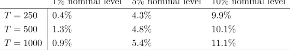
Tables 1 reports the size (i.e. the rejection frequencies under the null) of the bootstrap versions of theLRT test when we test forHR(1). From these results, we see that for moderate
and large sample sizes (T = 500and1000) the bootstrap test have very good size properties for both null hypohteses. In smaller sample sizes (T = 250), the size begin to deteriorate but is still acceptable.
1%nominal level 5%nominal level 10% nominal level
T = 250 0.4% 4.3% 9.9%
T = 500 1.3% 4.8% 10.1%
T = 1000 0.9% 5.4% 11.1%
Table 1: Size of bootstrap version ofsupLRT test for HR(1) : = 0.
The corresponding size performance for the LRT test of HR(2) are reported in Table 2.
Qualitatively the same picture as for the test of HR(1) appears: For moderate and large samples, the size is good while in smaller samples it is less precise.
1%nominal level 5%nominal level 10% nominal level
T = 250 0.4% 4.7% 11.8%
T = 500 1.0% 5.3% 11.7%
T = 1000 1.3% 6.3% 11.7%
Table 2: Size of bootstrap version ofLRT test for HR(2): = (1; 1).
Next, we examine the power of theLRT test for the two hypotheses. The results forHR(1)
are reported in Table 3 The test tends to have low power in small samples, and for example only rejects the incorrect hypothesis of = 0 with 16% probability for T = 250. However, as the sample size grows, the power quickly improvves and with T = 500 observations the bootstrap test exhibit acceptable power properties; for example, it rejects the incorrect null of = 0 with 67.6% probability at a 5% level. In large samples (T = 1000), the power is very good for the sup-test with rejection probabilities close to 100%.
1%nominal level 5%nominal level 10% nominal level
T = 250 2.7% 16.0% 29.2%
T = 500 37.5% 67.6% 78.1%
T = 1000 93.5% 97.0% 97.8%
Table 3: Power of bootstrap version ofsupLRtest for H0(1): = 0.
The power of the test of HR(2) is not quite as impressive as can be seen in Table 4. For example, it rejects at a 5% level with probability 49.5% and 76.4% for sample sizes of T = 500 and T = 1000 which is signi…cantly lower than the corresponding rejection probabilities reported in Table 3. This is to some extent probably a consequence of the DGP, which under the alternative of HR(2) is not too far away from the null with 0 having
been chosen as 0 = (1; 0:9282)0, cf. Appendix E. Hence it is more di¢ cult to detect the
departure from the null in …nite samples.
1%nominal level 5%nominal level 10% nominal level
T = 250 3.8% 17.0% 29.7%
T = 500 23.2% 49.5% 63.2%
T = 1000 63.5% 76.4% 81.4%
Table 4: Power of bootstrap version of LRT test for H0(2) : = (1; 1).
7
Conclusion
We have here proposed and analyzed likelihood-based estimators and tests in a class of nonlinear vector error correction models. The properties of estimators and tests prove to be non-standard in two distinct ways: First, due to the dependence between short- and long-run parameter estimators, their asymptotic distributions are not comparable to the standard Dickey-Fuller type asymptotics found in linear models. This in term a¤ects the test statistics. For example, tests only involving short-run parameters will in general not follow 2 in contrast to the situation in the linear cointegration model. The distribution of the test statistics get even more involved in the case of testing for linearity of the error correction mechanism due to vanishing parameters under the null.
Due to the complicated nature of the distributions, we proposed to implement the tests using a wild bootstrap procedure, and through simulations we demonstrated that the result-ing class of tests perform well both in terms of size and power. It would be of interest to show theoretically that the bootstrap procedure is consistent.
References
Andrews, D.W.K. and M. Buchinsky (2001) A Three-Step Method for Choosing the Number of Bootstrap Repetitions.Econometrica 68, 23-51.
Andrews, D.W.K. and W. Ploberger (1994) Optimal Tests When a Nuisance Parameter Is Present Only Under the Alternative. Econometrica 62, 1383-1414.
Andrews, D.W.K. and W. Ploberger (1995) Admissibility of the Likelihood Ratio Test When A Nuisance Parameter Is Present Only Under the Alternative. Annals of Statistics 23, 1609-1629.
Bec, F. and A. Rahbek (2004) Vector Equilibrium Correction Models with Non-linear Dis-continuous Adjustments. Econometrics Journal 7, 628-651.
Bickel, P.J. and M.J. Wichura (1971) Convergence Criteria for Multiparameter Stochastic Processes and Some Applications. Annals of Mathematical Statistics 42, 1656-1670. Brown, B.M. (1971) Martingale Central Limit Theorems. Annals of Mathematical Statistics
42, 59-66.
Caner, M. and B. Hansen (2001) Threshold Autoregression with a Unit Root.Econometrica
69, 1555–1596.
Cavaliere, G., A. Rahbek and R. Taylor (2010a) Testing for Cointegration in Vector Autore-gressions with Non-Stationary Volatility. Journal of Econometrics 158, 7-24.
Cavaliere, G., A. Rahbek and R. Taylor (2010b) Co-integration Rank Tests under Conditional Heteroskedasticity. Forthcoming in Econometric Theory.
Choi, I. and P. Saikkonen (2004) Testing Linearity in Cointegrating Smooth Transition Re-gressions.Econometrics Journal 7, 341–365.
Davies, R.B. (1987) Hypothesis Testing when a Nuisance Parameter is Present only under the Alternative. Biometrika 74, 33-43.
Doukhan, P., P. Massart and E. Rio (1995) Invariance Principles for Absolutely Regular Empirical Processes. Annales de l’Insitute Henri Poincaré 31, 393-427.
Gonzalo, J. and J.-Y. Pitarakis (2006) Threshold E¤ects in Multivariate Error Correction Models. In Palgrave Handbook of Econometrics: Econometric Theory (eds. T.C. Mills, K. Patterson), Vol. 1, 578-609.
de Jong, R.M. (2001) Nonlinear Estimation Using Estimated Cointegrating Relations. Jour-nal of Econometrics 101, 109-122.
de Jong, R.M. (2002) Nonlinear Minimization Estimators in the Presence of Cointegrating Relations. Journal of Econometrics 110, 241-259.
Hall, P. and C.C. Heyde (1980) Martingale Limit Theory and its Applications. New York: Academic Press.
Hansen, B.E. (1992) Convergence to Stochastic Integrals for Dependent Heterogeneous Processes. Econometric Theory 8, 489-500.
Hansen, B.E. (1996) Inference when a Nuisance Parameter is not Identi…ed under the Null Hypothesis. Econometrica 64, 413-430.
Hansen, B.E. and B. Seo (2002) Testing for Two-regime Threshold Cointegration in Vector Error Correction Models.Journal of Econometrics 110, 293-318.
Johansen, S. (1992) Estimation and Hypothesis Testing of Cointegration Vectors in Gaussian Vector Autoregressive Models. Econometrica 59, 1551-1580.
Johansen, S. (1996)Likelihood-Based Inference in Cointegrated Vector Autoregressive Models, 2nd Ed. Oxford: Oxford University Press.
Kapetanios, G. Y. Shin and A. Snell (2006) Testing for Cointegration in Nonlinear Smooth Transition Error Correction Models. Econometric Theory 22, 279–303.
Kilic, R. (2009) Testing for Co-integration and Nonlinear Adjustment in a Smooth Transition Error Correction Model. Manuscript, Georgia Institute of Technology.
Kristensen, D. and A. Rahbek (2005) Asymptotics of the QMLE for a Class of ARCH(q) Models,Econometric Theory 21, 946-961.
Kristensen, D. and A. Rahbek (2009) Asymptotics of the QMLE for Non-linear ARCH Models.Journal of Time Series Econometrics 1(1), Article 2.
Kristensen, D. and A. Rahbek (2010) Likelihood-Based Inference for Cointegration with Nonlinear Error-Correction. Journal of Econometrics 158, 78-94.
Kurtz, T.G. and P. Protter (1991) Weak Limit Theorems for Stochastic Integrals and Sto-chastic Di¤erential Equations. Annals of Probability 19, 1035-1070.
Magnus and Neudecker (1988) Matrix Di¤ erential Calculus with Applications in Statistics and Econometrics. New York: Wiley.
Meitz, M. and P. Saikkonen (2009) Parameter estimation in nonlinear AR-GARCH models. Working paper, University of Helsinki.
Nedeljkovic, M. (2008) Testing for Smooth Transition Nonlinearity in Adjustments of Coin-tegrating Systems, manuscript, Department of Economics, University of Warwick. Pitarakis, J.-Y. (2008) Comment on: Threshold Autoregression with a Unit Root.
Econo-metrica 76, 1207–1217.
Rahbek, A. H.C. Kongsted and C. Jørgensen (1999) Trend Stationarity in the I(2) Cointe-gration Model. Journal of Econometrics 90, 265-289.
Saikkonen, P. (2005) Stability Results for Nonlinear Error Correction Models. Journal of Econometrics 127, 69-81.
Saikkonen, P. (2008) Stability of Regime Switching Error Correction Models under Linear Cointegration. Econometric Theory 24, 294-318.
Seo, M.H. (2006) Bootstrap Testing for the Null of no Cointegration in a Threshold Vector Error Correction Model. Journal of Econometrics 134, 129–150.
Seo, M.H. (2008) Unit Root Test in a Threshold Autoregression: Asymptotic Theory and Residual-Based Block Bootstrap. Econometric Theory 24, 1699–1716.
Seo, M.H. (2010) Estimation of Nonlinear Error Correction Models. Forthcoming in Econo-metric Theory.
Straf, M.L. (1972) Weak Convergence of Stochastic Processes with Several Parameters. In
Proceedings of the Sixth Berkeley Symposium on Mathematical Statistics and Probability, Vol. 2, 187-221. University of California Press.
A
Proofs of Section 3
Proof of Theorem 3.4. Note initially that …nite dimensional convergence follows by stan-dard Martingale CLT results, see e.g. Brown (1971). In particular, ( T(s; ); T(~s;~))!D
( (s; ); (~s;~)) for any (s; ) and (~s;~) in [0;1] . Next, we show stochastic equicon-tinuity (tightness) by verifying the conditions of Theorem 3 in Bickel and Wichura (1971). Some further notation is needed for this: With s2[0;1]and 2 Rd ;let = (s; ) = (s; 1; :::; d ) and ~ = (~s;~) = ~s;~1; :::;~d be two arbitrary points in [0;1] . With
~ > , de…ne yT on( ;~), see Bickel and Wichura (1971),
T( ;~) := X 0=0;1 X 1=0;1 X d =0;1 ( 1)d +1 dj=0 j T(s 0ds; 1 1d 1; :::; d d d d );
whereds= (s s~)andd i = ( i ~i):Direct insertion gives that T ( ;~)can be written
as, T ( ;~) = 1 p T [Ts~] X t=[T s] ft( ;~)et; (A.1) where ft( ;~) = X 1=0;1 X d =0;1 ( 1)d dj=1 jf(y t 1; 1 1d 1; :::; d d d d ): (A.2)
Since (s; ) 7! (s; ) is almost surely continuous, then by Straf (1972, Theorem 5.6) in combination with Bickel and Wichura (1971, Theorem 1) it su¢ ces to establish that, for someq >0; >1,
Ek T( ;~]k2q Cjs~ sj i=1;2;::;d j~i ij : (A.3)
Under Assumptions 3.1-3.2, and using Rosenthal’s inequality (see Hall and Heyde, 1980, p.23), Cauchy-Schwarz, and eq. (A.1), it follows that forq >1,
Ek T( ;~)k2q C Tq 0 @ [T~s] X t=[T s] EhE ketk2k ft( ;~)k2jFt 1 i1 A q + C Tq [T~s] X t=[T s] Ehketk2qk ft( ;~)k2q i C [Ts~] [T T s] qk ekq Ek ft( ;~)k2 q +C [Ts~] [TqT s] h Eketk4q Ek ft( ;~)k4q i1=2 C [Ts~] [T T s] qEk ft( ;~)k2q+o(1); (A.4)
asT ! 1. Observe that for eachi2D =f1; :::; d g, one may write ft( ;~]as,
ft( ;~) =
X
j2D ; ;j6=i; "j=0;1
( 1)d j6=i"j@
where@ift( ;~]denotes the increments off( )over the ith coordinate of ,
@ift( ;~) =ft( 1 1d 1; :::; i 1 i 1d i 1;~i; i+1 i+1d i+1; :::; q qd d )
ft( 1 1d 1; :::; i 1 i 1d i 1; i; i+1 i+1d i+1; :::; q qd d );
withd i = ~i i:Using eq. (A.5), and by Assumption 3.2,
Ek ft( ;~)k2 C2d 1Ek@ift( ;~]k2 Cj~i ij2
As this holds for each i, one gets that forT large enough, eq. (A.4) is bounded by,
Ek T( ;~)k2q Cjs~ sjq Ek ft( ;~)k2 q
Cjs~ sjq i2D j~i ij2 q=d ;
and the desired holds.
Proof of Corollary 3.7. For …xed s the result holds by Doukhan et al (1995), see also
Hansen (1996), while for …xed the result holds by Brown (1971).
Proof of Theorem 3.5. It follows by standard results that the convergence holds for any given 2 , see e.g. Kurtz and Protter (1991, Theorem 2.2). Proceeding as in the proof of Theorem 3.4, de…ne VT ( ) = 1 p T T X t=1 x0t 1f(yt 1; )et; VT ( ;~) = 1 p T T X t=1 x0t 1 ft( ;~)et;
where ft is de…ned in eq. (A.2). Again by Rosenthal’s inequality (Hall and Heyde, 1980,
p.23) and Cauchy-Schwarz inequalities, forn >1,
Ehk VT( ;~)k2q i C Tq T X t=1 EhE kxt 1k2ketk2k ft( ;~)k2jFt 1 i!q + C Tq T X t=1 E kxt 1k2qketk2qk ft( ;~)k2q Ck ekq sup t Ekxt 1k4 Ek ft( ;~)k4 q=2 +CT1 qE sup t k xt 1k2qketk2qk ft( ;~)k2q Ck ekq sup t Ekxt 1k4Ek ft( ;~)k4 q=2 +CT1 q Esup t k xt 1k6qEketk6qEsup 2 k f(yt 1; )k6q 1=3 C i2D j~i ij2 q=d +o(1):
By the same arguments as employed in the proof of Theorem 3.4, the desired result now follows.
Proof of Theorem 3.6. De…ne the mean-zero sequenceut( ) =f(yt 1; ) E[f(yt 1; )] and write 1 T PT t=1x0t 1f(yt 1; ) = 1 T PT t=1x0t 1E[f(yt 1; )] + 1 T PT t=1x0t 1ut( ):
By Assumption 3.3 and the Continuous Mapping Theorem, the …rst term converges towards the claimed limit. We then need to show that the second term goes to zero in probability uniformly in . We follow the same arguments as in Caner and Hansen (2001, Proof of Theorem 3): For any given >0, de…ne N = [1= ], tk = [k T] + 1 and tk =tk+1 1, and
write 1 T T X t=1 x0t 1ut( ) = 1 T NX1 k=0 tk X t=tk xt 10ut( ) = 1 T NX1 k=0 tk X t=tk (xt 1 xtk 1) 0u t( ) + 1 T NX1 k=0 x0t k 1 tk X t=tk ut( ):
The …rst term is bounded by, 1 T NX1 k=0 tk X t=tk kxt 1 xtk 1ksup 2 k ut( )k ( sup jt t0j T k xt xt0k ) 1 T NX1 k=0 tk X t=tk sup 2 k ut( )k;
where, by the law of large numbers, 1 T NX1 k=0 tk X t=tk sup 2 k ut( )k= 1 T T X t=1 sup 2 k ut( )k P !E sup 2 k ut( )k <1; and, by Assumption 3.3, sup jt t0j T k xt xt0k!D sup js s0j x(s) x s0 :
The limit can be made arbitrarily small due to a.s. continuity ofx(s). The second term is bounded by 1 T NX1 k=0 kxtk 1k tk X t=tk ut( ) ( sup 1 t Tk xtk ) 1 T NX1 k=0 tk X t=tk ut( ) ;
where sup1 t Tkxtk = OP(1). Next, sup 2 jjPNt=1ut( )=Njj P
! 0 by Kristensen and Rahbek (2005, Proposition 1) as N ! 1, and hence the arguments following (A.10) in Caner and Hansen (2001, proof of Theorem 3) imply that
sup 2 1 T NX1 k=0 tk X t=tk ut( ) !P 0; asT ! 1:
B
Proofs of Section 4
Proof of Lemma 4.5. Choose any d , d and d and de…ne = vec(d ; d ; d ). We
consider the sequence
T(s; ) := 1 p T [T s] X t=1 0 uut( ) + 0vvt( ) + 0wwt( ) = 1 p T [T s] X t=1 f(yt 1; )et; withet:= 01"t,yt 1= Z00;t 1; Z20;t 1 0, and f(yt 1; ) := [d Z0;t 1+d (Z0;t 1; ) +d Z2;t 1]0:
Also note that = . Here, by Assumption 4.1
kf(yt 1; )k c(kZ0;t 1k+k (Z0;t 1; )k+kZ2;t 1k) c(kZ0;t 1k+kZ0;t 1k +kZ2;t 1k)
Thus,
kf(yt 1; )km c(kZ0;t 1km+kZ0;t 1km +kZ2;t 1km):
Furthermore, by the di¤erentiability of ,
E f(yt 1; ) f yt 1; 0 n =E (Z0;t 1; ) Z0;t 1; 0 n E " @ Z0;t 1; @ n# 0 n E[kZ0;t 1k n] 0 n ;
such that = 1. Thus, the requirement n > 2 translates into EhkZ0;t 1k(2+ )
i
< 1 for some >0, and the requirementm > m:= max (4;2d )translates intoE kZ0;t 1km <1
with = max (1; ), and E kZ2;t 1km <1.
This veri…es that Assumptions 4.2-4.4 imply that the Assumptions 3.1-3.3 of Theo-rem 3.4 hold, and hence the result follows for (u0t( ); vt0( ); w0t( )). The joint convergence holds by the marginal convergence in Assumption 4.3, in conjunction with the fact that (u0
t( ); v0t( ); w0t( ))and Xt are de…ned in terms of ("s)s t.
Proof of Theorems 4.6. For ease of notation, we treat = 0 as known such that
LT = LT. The extension to unknown is straigthforward and follows along the lines of
Kristensen and Rahbek (2010).
To establish the result, we apply a general formulation in Lemmas D.1 and D.2 in Appen-dix D below which will allow us to consider convergence uniformly in . To use the results in Section D, set =vec(#), = 0; QT( ; ) =QT (#) = T1LT(#), with LT (#) de…ned in
eq. (2.11), vT =T and UT =VT, whereVT is de…ned in eq. (4.3). To prove consistency, we
verify the conditions of Lemma D.1: We have that condition (i) holds by Assumption 4.1, while (ii)-(iii) follow by Lemmas C.1, C.2 and C.3:
dQT(#0; 0;UT1=2d ) =
1
TdLT(#0;V 1=2