Machine Learning techniques for energy consumption forecasting in Smart Cities scenarios

(1)

CAPSI 2020 Proceedings Portugal (CAPSI)

10-2020

Machine Learning techniques for energy consumption forecasting

in Smart Cities scenarios

Francisco Sério

Filipe Pinto

Cristina Wanzeller

Follow this and additional works at: https://aisel.aisnet.org/capsi2020

This material is brought to you by the Portugal (CAPSI) at AIS Electronic Library (AISeL). It has been accepted for inclusion in CAPSI 2020 Proceedings by an authorized administrator of AIS Electronic Library (AISeL). For more information, please contact [email protected].

(2)

20.ª Conferência da Associação Portuguesa de Sistemas de Informação (CAPSI’2020) 16 e 17 de outubro de 2020, Porto, Portugal

ISSN 2183-489X

1

Francisco Sério, Filipe Cabral Pinto, Cristina Wanzeller

CISeD – Research Centre in Digital Services, Polytechnic of Viseu, Portugal [email protected], [email protected], [email protected]

Abstract

Over the past few years, the number of sensors spread across cities has significantly increased. This led to an exponential growth in data volume, which can only be treated with Big Data techniques. Having such a large amount of generated data, turns possible to apply machine learning techniques more accurately, with the goal of making data predictions over time, finding anomalies, performing classification, among other tasks. This article aims to show the application of machine learning techniques, using a variant of the Recurrent Neural Networks, the Long Short-Term Memory (LSTM), in order to predict city's energy consumptions for the near future. This forecast will support municipal entities decisions, helping them to improve the managing of energy consumptions and budgets.

Keywords: Machine Learning, Smart Cities, Internet of Things, Big Data, LSTM

1. I

NTRODUCTION

Currently, electric energy is an essential asset for everyone. It is used in our homes, through electronic equipment and lighting, and also in agriculture, industry, public lighting and other varied forms in cities.

The fast urbanization of cities and the growth of the population, tend to hinder the energy consumptions management (Ejaz, Naeem, Shahid, Anpalagan and Jo, 2017). Solving this problem, will help counties to achieve proposed sustainability goals, which some are obligated to comply, improving the general quality of life of their population. Consequently, municipalities would have a greater view of their economy, being able to reduce costs in some areas. Moreover, this would result in a performance improvement in other domains, such as health and education (Pérez-Chacón, Luna-Romera, Troncoso, Martínez-Álvarez and Riquelme, 2018).

A possible solution to the presented problem is the use of Machine Learning (ML) algorithms in energy data to predict consumptions, for the near future. This is not exactly a new topic: currently, the scenario where this is most used is not in a cities’ context, but in buildings’ energy consumption or other isolated premises. A city scenario involves more challenges, since there are multiple factors that can influence these forecasts, such as temperature and air quality.

(3)

20.ª Conferência da Associação Portuguesa de Sistemas de Informação (CAPSI’2020) 2

Forecasting energy consumptions in cities was not as easy to perform as it is today, due to the lack of data from partners. Currently, there are already several devices of all types providing data. For example, smart meters, present information about the energy consumption in a web page. Every user of such devices can access data through their personal account (Lima, 2015).

In order to make accurate use of ML possible, concerning energy consumption data, and also data from other types of sources, a large data set is necessary. Having plenty of data, the algorithm can train, recognize patterns and be prepared for specific forecasts required by the user, providing the forecasts with lower percentage of error.

However, large amounts of data (Big Data), in itself, may not be totally advantageous for machine learning, if the data has no quality. Sometimes it is preferable, for example, to discard some of the data attributes than use them all and even add some more, so that the algorithm obtains a better result. Therefore, the importance of data mining and data science (Sessions and Valtorta, 2006). This article aims to show the application of Machine Learning techniques on real energy consumption data from a city, with the goal of forecasting consumptions in the near future. The studies conclude that the county is able to take better decisions based on these forecasts, as well as to better manage its resources, avoiding waste and over-reaching their expectations.

Also, with this project, it is intended to contribute in the scientific community, with regard to the forecast of energy consumptions, in smart cities’ scenarios.

The paper is organized as follows. Section 2 summarizes the state of the art, describing the concepts of Smart Cities, Internet of Things, Big Data, Machine Learning and Long Short-Term Memory. This section also describes appropriate related work. Section 3 details the various steps of the experimental setup, starting with the data set used, the feature engineering applied, the construction of the model and its evaluation. Section 4 presents the conclusions of the article.

2. S

TATE OF ART

In this new era of Smart Cities, there are several interconnected areas, working together to obtain a single result. This is the case of the areas mentioned in the next sections.

2.1. Smart Cities

Over the past few years, the concept of Smart Cities has been appearing more frequently, and the trend is to rise more and more. As Bolívar (2015) says, in recent years, cities managers are increasingly aware of the Smart City concept and developing several methods with the aim of turning the cities intelligent on their own and offering more efficient control over the cities.

(4)

Currently, there are several definitions about this concept that appeared for the first time in 1998 (Anthopoulos, 2015). According to Su, Li and Fu (2011), a smart city is a specific region, in which information and integrated management of the city are carried out. Further, from the same source, it can also be said that it is an intelligent and effective integration of planning ideas, modes of construction, management methods and development approaches. On the other hand, with the arrival of the concept of “Internet of Things” (IoT), Arasteh et al (2016) say that a smart city is equipped with different electronic devices, for different applications, such as, for example, surveillance cameras placed on the streets and sensors for transport systems, thus showing the importance of IoT in a smart city.

With the rapid growth of the population in recent years and the constant migration of them from the countryside to the urban area, many cities are having problems related to their sustainability, affecting the citizens’ lives. Some of the problems are in waste management, air pollution control, traffic congestion, deterioration of buildings, among many others (Chourabi et al, 2012).

In order to solve such kind of problems, many cities have created initiatives and projects, not only to improve the quality of life of their inhabitants, but also to meet sustainability goals imposed on them (Arroub, Zahi, Sabir and Sadik, 2016).

2.2. Internet of Things and Big Data

Like Smart Cities, the Internet of Things (IoT) and Big Data are two concepts that have appeared more frequently over the past few years and, due to that, several meanings have appeared.

According to Patel and Patel (2016), IoT is like a network of devices that are connected, where the information produced by them can be accessed by everyone, anytime and anywhere. Madakam, Ramaswamy and Tripathi (2015) say that IoT is a technological revolution, representing the future of computing and communications, from wireless sensors to nanotechnology, with the aim of control these technological innovations and monitoring the information flow produced by them, even in real time.

About Big Data, De Mauro, Greco and Grimaldi (2016) think that it is a large amount of information characterized by its volume, velocity and variety. So, knowledge from other areas, such as Data Science and Data Mining, is needed to get the real value from that information. With a similar idea, Youssra and Sara (2018) state that Big Data refers to large diversified data sets, consisting of structured, semi-structured and unstructured data, where they are increasingly arriving data more quickly, mentioning the three “V's” once again: Volume, Velocity and Variety.

Over time, these two terms have been increasingly directly related. De Mauro, A. Et al (2016) even say that IoT generates Big Data for several reasons. One of them is the speed associated with the massive IoT devices’ production and the wide variety of data that different sensors produce daily,

(5)

generating more and more different kinds of data. This augment can have very positive consequences for some areas of information technology, mostly for Data Analytics and Machine Learning, because without a large amount of data, these two areas are unable to give the user the best results (Bomatpalli and Vemulkar, 2016).

2.3. Machine Learning

Machine learning is a concept that has been gaining more importance in the last years, due to the increase of data. It has been applied to several areas, such as health, industry, agriculture, among others.

According to El Naqa and Murphy (2015), machine learning is a branch of computational algorithms with the aim of simulating the human intelligence that learns with the environment that surrounds it. With a similar idea, Surden (2014) says that machine learning is a branch of artificial intelligence where the computer system can learn from experience, improving its performance in some tasks over time.

A generic framework for cognitive cities was proposed by Carvalho, Pinto, Borges, Machado and Oliveira (2019). Machine Learning techniques were applied to enhance the city management by predicting behaviors and automatically adapt rules mechanisms in order to mitigate city problems. The application of Machine Learning in electricity consumption has been widely used, especially in buildings, such as schools, personal houses and skyscrapers, due to the growing number of IoT devices present in the markets.

Currently there are several machine learning algorithms, each for its own purpose, type of problem and data. In the case of energy consumption forecasting, in most cases, data are associated with the time they were collected, which means that the data sets are time series. One of the models that, for this type of scenarios, has obtained better results is called the Artificial Neural Network (ANN) (Siami-Namini, Tavakoli and Namin, 2018).

ANNs, over the last few years, have been widely used, due to their ability to solve complex classification problems and time series.

This model is based on the Human brain and nervous system, as can be seen in Figure 1. In a neural network, the neuron of a human brain is represented by a neuron, which is basically a mathematical expression. These neurons together form the neural network, where each receives input values. These values are multiplied by their weights, passing, finally, to an activation function, producing a final value. This value passes to the next layer, repeating the process in all neurons until reaching the final layer, called Output layer, which will generate the set of output values (Walczak and Cerpa, 2003).

(6)

Figure 1 – Example of a typical neural network1

In a typical ANN, two successive inputs are independent of each other. However, there are scenarios where the inputs depend on the previous ones. For example, for forecasting the price of a stock, based on time or predicting the next word in a given sequence, ANNs are not the most suitable. For these types of problems, there are the Recurrent Neural Networks (RNN), where each layer is dependent on the previous one, allowing the cell to have a kind of memory. However, this kind of neural network has the problem of vanishing gradient and exploding gradient. So, in practice, they are difficult to train when it is necessary to memorize a large amount of previous sequential data. To solve this problem, a variant of the RNN, called Long Short-Term Memory, was created (Yue, Fu and Liang, 2018).

2.4. Long Short-Term Memory (LSTM)

LSTM networks are a specific kind of Recurrent Neural Networks, created to solve the problem mentioned in the previous section. These neural networks are one of the most used over the past few years, especially to solve problems where data are sequential, such as speech recognition, stock forecasting, among others (Fischer and Krauss, 2018).

The architecture of an LSTM cell, which is represented in Figure 2, consists of 3 gates (Forget gate, Input gate and Output gate) and 2 cells, one of memory (Memory) and another of state (Hidden state).

(7)

Figure 2 –LSTM architecture2

The Forget gate is responsible for removing information from the State cell, which is the output of the previous unit. This is an important operation to optimize the performance of the neural network, because it eliminates information that is no longer needed or that has no longer importance. The Forget gate (Ft) is defined by the following expression (1), where σ is the sigmoid activation

function, Xt is the input at a given time, the Wxf and Whf the weights of the matrices, the Ht−1 the

Hidden State and o bf the bias:

Ft= σ (XtWxf + Ht−1Whf + bf) (1)

The Input gate (It) is responsible for adding information to the State cell. This gate has two parts:

the first (2) is similar to the Forget gate, where it filters all the information from the State cell and the Input and the second (3), where it transforms that information into a vector and adds it to the State cell ( Hu and Balasubramaniam, 2008).

It= σ (XtWxi + Ht−1Whi + bi) (2)

Ct= tanh (XtWxc + Ht−1Whc+ bc) (3)

Output gate (Ot) selects useful information from the current State cell (4). Then, the tangent

hyperbolic (tanh) activation function is applied in order to create a vector with values between -1 and +1 (5) (Kim, Kim, Thu and Kim, 2016).

Ot= σ (XtWxo + Ht−1Who + bo) (4)

Ht = Ot*tanh (Ct) (5)

2.5. Related works

The idea of forecasting energy consumptions is not exactly new. Many researchers have tried to find the algorithm with the lowest percentage of error in forecasting this kind of time based data.

(8)

Edwards, New and Parker (2012), having data from sensors in three residential buildings, applied machine learning algorithms to predict the energy consumptions of buildings for the next hour, with very positive results, mostly for the LS-SVM (Least-squares Support-vector Machine).

In a similar project, Ahmad, Mourshed and Rezgui (2017) used two ML algorithms, ANN and

Random Forest (RF), to predict energy consumptions in buildings. In this work, a hotel data set was used to make consumption forecasts for the next hour. The algorithm with the best results was ANN.

On the other hand, Seyedzadeh, Rahimian, Glesk and Roper (2018) compared four of the most

well-known ML models for predicting the consumption of electrical energy in buildings. The models are: Artificial Neural Network, Support Vector Machine (SVM), Gaussian-based Regression and Clustering. With this research, it was concluded that all these models have their advantages and disadvantages, depending on the type of data and the input variables.

Amasyali and El-Gohary (2016) used the SVM algorithm to forecast building lighting consumptions. In these forecasts, the variables used were the type of day and the sky coverage. This work allows to conclude that this algorithm can be applied, successfully, in the prediction of lighting energy consumptions.

Vinagre, Pinto, Ramos, Vale and Corchado (2016) used, once again, the SVM algorithm to predict the energy consumption of a building. The data was collected every 10 seconds and used to forecast energy consumption on the last Friday of each month. This experience showed that it is possible to use this algorithm to predict this kind of data, in complex scenarios, even with better results than ANN algorithm.

3. E

XPERIMENTAL

S

ETUP

In the following sections, some ML techniques are presented, as well as the steps applied in an experimental work. This work aims to build a model for making predictions of energy consumptions in a city, using the LSTM.

3.1. Dataset

Finding a dataset from an entire city is a real challenge, because what is usually found are datasets

about buildings and houses. There is also the question of data confidentiality, where many companies

are not comfortable providing data for studies.

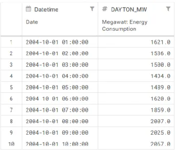
The data set chosen for the forecast of energy consumptions was the PJM Hourly Energy Consumption Data, from the city of Dayton (Ohio, United States of America). This data set is freely available by the PJM Interconnection organization. Figure 3 shows the first 10 rows of the data set.

(9)

20.ª Conferência da Associação Portuguesa de Sistemas de Informação (CAPSI’2020) 8 This data set has 2 columns, the first referring to the collection date of each reading and the second

to energy consumptions, in Megawatts. Data was collected since 2004, which is good for training

ML models, because they usually require a lot of data and, since the forecast is based on time, it is important that the dataset has data over several years, what makes this dataset a great choice for this article.

Figure 3 – Data set used

It can be said that this data set is a univariate time series, because it only presents a single attribute which is, in this case, the energy consumption column.

For a better visualization of the data set, a graph with the total data is shown in Figure 4, where the X axis represents the date of data collection and the Y axis the measures, in Megawatt.

(10)

20.ª Conferência da Associação Portuguesa de Sistemas de Informação (CAPSI’2020) 9 3.2. Feature Engineering

As stated in the previous section, the data set is a univariate time series. In order to generate a greater number of attributes, the feature engineering was made. This is a process of using the domain of knowledge of the data to create attributes, which may be used in ML as inputs. Using feature engineering, it is possible to get a greater knowledge of the data set and helps in the model validation (Zaidi, 2015).

Through the column of time (Datetime), the columns “dayofweek”, “year”, “month”, “day” and “hour” were created, representing the day of the week, the year, the month, the day and the hour in which energy consumptions data were collected, respectively.

These attributes were chosen because they are directly related to the increase of energy consumptions, as can be seen in Table 1. The table shows the variation of the average consumption depending on the day of the week.

DAYOF THE WEEK ENERGY CONSUMPTION (MEGAWATT)

Monday 2100.55

Tuesday 2146.55

Wednesday 2146.07

Thursday 2136.36

Friday 2085.28

Table 1 – Average electricity consumption grouped by day of the week

Checking the results, it can be concluded that from Monday to Friday, the average of the energy consumptions is higher than on Saturday and Sunday. These numbers can be considered within the normal band, because, on weekdays, for example, in the case of information technology companies, they spend more energy due to the use of computers, monitors, printers, among other equipment. At weekends, these companies are normally closed and that’s why there is a decrease in the average of energy consumptions.

This kind of information is also important for the validation of the model. Considering the previous example, if, for example, a forecast of a data whose day of the week is “Tuesday” and has a consumption less than 2000 Megawatt, is possible to conclude that this forecast is probably wrong.

3.3. Model

The python programming language was used for the construction of the model, because there is a large community using it in the ML area. As a backend, were used the Tensorflow 2.0 and the Keras library, which offers an easy application programming interface (API) for several models, including LSTM.

(11)

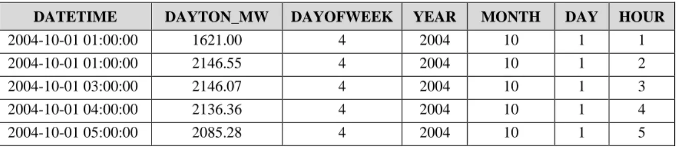
Having the feature engineering performed, presented in the previous section, the final data set has a total of 7 columns, as shown in Table 2. The first column refers to the date when each energy consumption data was collected. This column was converted as an index of the table because it is a time series. The other 6 columns are the attributes that will be used in the model.

DATETIME DAYTON_MW DAYOFWEEK YEAR MONTH DAY HOUR

2004-10-01 01:00:00 1621.00 4 2004 10 1 1 2004-10-01 01:00:00 2146.55 4 2004 10 1 2 2004-10-01 03:00:00 2146.07 4 2004 10 1 3 2004-10-01 04:00:00 2136.36 4 2004 10 1 4 2004-10-01 05:00:00 2085.28 4 2004 10 1 5

Table 2 – Data set with the first 5 rows

For the data pre-processing, it was not necessary any kind of data cleaning technique, such as removing data with null values and changing data that are outside the normal range of the set, because the data set had all the data in the correct form and in the normal range. The only operations performed were the ordering of the data, in ascending order of the data collection date, and the normalization of the data with an interval between 0 and 1. This assures that the data can be within the same interval, to prevent the algorithm going the wrong direction due to the difference in the value of each data.

For the future validation of the model, the data set was divided into training and test. The percentage chosen was 75% for training and 25% for test. Because it is a time series, the collection date matters and, therefore, the training data were the first 75% and the test data were the remaining 25% of the data set (Reitermanova, 2010).

To use the API of the LSTM model, the Keras library requires an input format of a three-dimensional vector, where the first dimension is the number of data set rows (samples), the second represents the number of data that the neural network will have to remember (time steps) and the last one refers to the number of data set attributes (Brownlee, 2018).

In the model, using, then, the Keras library, were used 4 layers, the first (input layer) with 128 memory cells, the next 2 layers (hidden layers) with the same number of memory cells and the last (output layer) with a single memory cell. The activation function used in each layer was the Tanh (hyperbolic tangent). At the end of each layer, a Dropout of 0.2 was used to prevent overfitting. This operator is very important, because it corrupts the information carried by the memory cells, forcing them to perform their intermediate calculations more robustly, preventing the neural network from “decorating” the data during training and offering incorrect predictions (Zaremba, Sutskever and Vinyals, 2014). The number of times used was 100 and the batch size was 64, which means that the neural network trains with 64 data at a time.

(12)

The number of layers, epochs, memory cells, dropout and the type of activation function were chosen precisely for this kind of data set. There is no general rule that says, for example, the ideal number of layers that a LSTM network must have. It is all about the type and quantity of the data set. Using the example of the number of layers chosen, if the data set had a higher level of complexity, it would be necessary a greater number of layers, so that the neural network could be able to know more complex patterns, which would imply that the network would take more time to train.

3.4. Model evaluation

Model evaluation was made by building models for 1, 10 and 100 periods and for two types of data sets: one with the original data set, which only has the attribute related to energy consumptions (univariate time series) and the other with the 6 attributes (multivariate time series), which was made after performing the feature engineering.

For both models, it was used the Root Mean Square Error (RMSE) for the evaluation, because it is one of the most common metrics for evaluating numerical predictions (Roondiwala, Patel and Varma, 2017). The Table 3 shows the comparison between the results of the two models.

EPOCHS UNIVARIATE TIME SERIES MULTIVARIATE TIME SERIES

1 474 68

10 349 22

100 197 11

Table 3 – Comparison between the results of the two models

As can be seen in the previous table, the multivariate time series got better results, because has a lower RSME. About the number of epochs, it can be said that in both models that had more epochs, had better results.

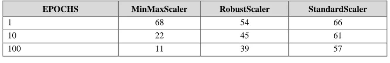
In order to compare which type of normalization would obtain better results, were built 3 more models with 3 of the most common types of normalization: MinMaxScaler (used in the previous models), RobustScaler and StandardScaler. For these models was used the multivariate data set. The Table 4 shows the comparation between the normalizations in 3 different epochs.

EPOCHS MinMaxScaler RobustScaler StandardScaler

1 68 54 66

10 22 45 61

100 11 39 57

(13)

Regarding to the previous table, it can be concluded that the MinMaxScaler normalization type got better results with a greater number of epochs, compared to the other 2 types.

Another important metric that deserves to be mentioned is the used activation function on the output layer. Were build models using 3 of the most used activation functions in ANNs: Tanh (used in the previous models), Sigmoid and ReLu. For these models was used the multivariate data set. The Table 5 shows the comparation between the activation functions in 3 different epochs.

EPOCHS Tanh Sigmoid ReLu

1 68 68 66

10 22 28 32

100 11 33 13

Table 5 – Comparison between the used activation functions

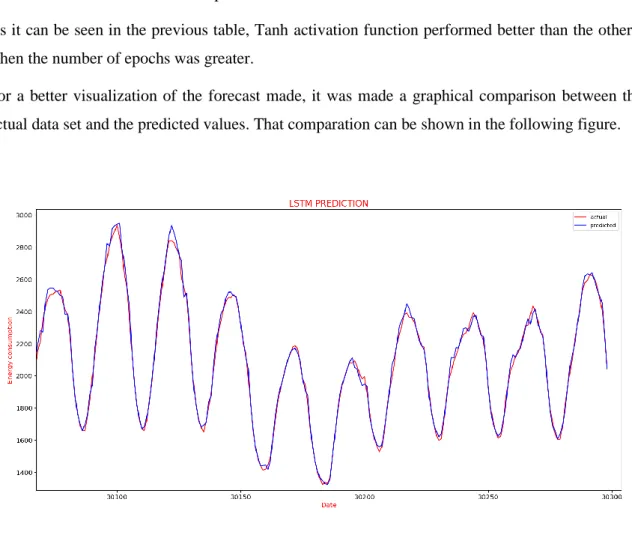
As it can be seen in the previous table, Tanh activation function performed better than the others, when the number of epochs was greater.

For a better visualization of the forecast made, it was made a graphical comparison between the actual data set and the predicted values. That comparation can be shown in the following figure.

Figure 5 – Last current and forecast data

Through the previous figure, it can be seen that the model was able to predict quite well, learning the different patterns that the data set had.

(14)

4. C

ONCLUSION

The developed work allows to conclude that the use of Long Short-Term Memory in the energy consumption data of a city, is, in fact, a good option to make predictions for the next future. One of the steps of the machine learning process that is, sometimes, undervalued is the feature engineering. Based on this work it is also possible to conclude that it is important to have a data set with more than one attribute for time series problems, in order to try to reduce the error and getting better results in the forecast.

It is important to note that the choice of the normalization type and the activation function on the output layer are important because some of these choices can obtain different results for other types of datasets.

One limitation of this article is the number of attributes that the original dataset offers. It would be interesting if it had attributes about, for example, temperature, because not only could offer a better result in the forecasts, but also could help in the data analysis process. It would also be interesting to test the model in datasets from other cities, to verify if it would forecast as well as for this dataset. As a future work, we intend to build machine learning models, using LSTM, on other types of data from smart cities, such as data related to waste, water and air quality, temperature, among others, with the goal of enabling the city to forecast different uses, allowing to offer optimized services, improving citizens’ lives.

5. A

CKNOWLEDGEMENTS

” This work is funded by National Funds through the FCT - Foundation for Science and Technology, I.P., within the scope of the project Ref UIDB/05583/2020. Furthermore, we would like to thank the Research Centre in Digital Services (CISeD), the Polytechnic of Viseu for their support.”

R

EFERENCES

Ahmad, M.W., Mourshed, M. & Rezgui, Y., 2017. Trees vs Neurons: Comparison between random forest and ANN for high-resolution prediction of building energy consumption. Energy and Buildings, 147, pp.77-89.

Amasyali, K. & El-Gohary, N., 2016. Building lighting energy consumption prediction for supporting energy data analytics. Procedia Engineering, 145, pp.511-517.

Anthopoulos, L.G., 2015. Understanding the smart city domain: A literature review. In Transforming city governments for successful smart cities (pp. 9-21). Springer, Cham.

Arasteh, H., Hosseinnezhad, V., Loia, V., Tommasetti, A., Troisi, O., Shafie-Khah, M. and Siano, P., 2016, June. Iot-based smart cities: a survey. In 2016 IEEE 16th International Conference on Environment and Electrical Engineering (EEEIC) (pp. 1-6). IEEE.

Arroub, A., Zahi, B., Sabir, E. & Sadik, M., 2016, October. A literature review on Smart Cities: Paradigms, opportunities and open problems. In 2016 International Conference on Wireless Networks and Mobile Communications (WINCOM) (pp. 180-186). IEEE.

Bolívar, M.P.R., 2015. Smart cities: Big cities, complex governance?. In Transforming city governments for successful smart cities (pp. 1-7). Springer, Cham.

(15)

20.ª Conferência da Associação Portuguesa de Sistemas de Informação (CAPSI’2020) 14 Bomatpalli, T. & Vemulkar, G. (2016). BLENDING IOT AND BIG DATA ANALYTICS.

INTERNATIONAL JOURNAL OF ENGINEERING SCIENCES & RESEARCH TECHNOLOGY, 5(4), 192-196.

Brownlee, J. (2018). Deep Learning for Time Series Forecasting: Predict the Future with MLPs, CNNs and LSTMs in Python. Machine Learning Mastery.

Chourabi, H., Nam, T., Walker, S., Gil-Garcia, J.R., Mellouli, S., Nahon, K., Pardo, T.A. & Scholl, H.J., 2012, January. Understanding smart cities: An integrative framework. In 2012 45th Hawaii international conference on system sciences (pp. 2289-2297). IEEE.

Carvalho, C., Pinto, F., Borges, I., Machado, G. & Oliveira, I. (2019). Cognitive Cities an Architectural Framework for the Cities of the Future. International Conference on Machine Learning & Applications. 173-182.

De Mauro, A., Greco, M. & Grimaldi, M., 2016. A formal definition of Big Data based on its essential features. Library Review, 65(3), pp.122-135.

Edwards, R.E., New, J. & Parker, L.E., 2012. Predicting future hourly residential electrical consumption: A machine learning case study. Energy and Buildings, 49, pp.591-603.

Ejaz, W., Naeem, M., Shahid, A., Anpalagan, A. & Jo, M., 2017. Efficient energy management for the internet of things in smart cities. IEEE Communications Magazine, 55(1), pp.84-91.

El Naqa, I. & Murphy, M.J., 2015. What is machine learning?. In Machine Learning in Radiation Oncology (pp. 3-11). Springer, Cham.

Fischer, T., & Krauss, C. (2018). Deep learning with long short-term memory networks for financial market predictions. European Journal of Operational Research, 270(2), 654-669.

Hu, X., & Balasubramaniam, P. (Eds.). (2008). Recurrent neural networks (Vol. 400). InTech. Kim, J., Kim, J., Thu, H. L. T., & Kim, H. (2016, February). Long short term memory recurrent neural

network classifier for intrusion detection. In 2016 International Conference on Platform Technology and Service (PlatCon) (pp. 1-5). IEEE.

Lima, C.M.N., 2015. Previsão de consumo de energia elétrica em contexto de smart grids (Doctoral dissertation).

Madakam, S., Ramaswamy, R. & Tripathi, S., 2015. Internet of Things (IoT): A literature review. Journal of Computer and Communications, 3(05), p.164.

Patel, K.K. & Patel, S.M., 2016. Internet of things-IOT: definition, characteristics, architecture, enabling technologies, application & future challenges. International journal of engineering science and computing, 6(5).

Pérez-Chacón, R., Luna-Romera, J., Troncoso, A., Martínez-Álvarez, F. & Riquelme, J., 2018. Big data analytics for discovering electricity consumption patterns in smart cities. Energies, 11(3), p.683.

Reitermanova, Z. (2010). Data splitting. In WDS (Vol. 10, pp. 31-36).

Roondiwala, M., Patel, H., & Varma, S. (2017). Predicting stock prices using LSTM. International Journal of Science and Research (IJSR), 6(4), 1754-1756.

Sessions, V. & Valtorta, M. (2006). The Effects of Data Quality on Machine Learning Algorithms. ICIQ, 6, 485-498.

Seyedzadeh, S., Rahimian, F.P., Glesk, I. & Roper, M., 2018. Machine learning for estimation of building energy consumption and performance: a review. Visualization in Engineering, 6(1), p.5. Siami-Namini, S., Tavakoli, N., & Namin, A. S. (2018). A comparison of ARIMA and LSTM in forecasting time series. In 2018 17th IEEE International Conference on Machine Learning and Applications (ICMLA) (pp. 1394-1401). IEEE.

Su, K., Li, J. & Fu, H., 2011, September. Smart city and the applications. In 2011 international conference on electronics, communications and control (ICECC) (pp. 1028-1031). IEEE. Surden, H., 2014. Machine learning and law. Wash. L. Rev., 89, p.87.

Vinagre, E., Pinto, T., Ramos, S., Vale, Z. & Corchado, J.M. (2016). Electrical energy consumption forecast using support vector machines. In 2016 27th International Workshop on Database and Expert Systems Applications (DEXA) (pp. 171-175). IEEE.

Walczak, Steven & Cerpa, Narciso. (2003). Artificial Neural Networks. 10.1016/B0-12-227410-5/00837-1.

Youssra, R. & Sara, R., 2018. Big data and big data analytics: concepts, types and technologies. Int J Res Eng, 5(9), pp.524-528.

Yue, B., Fu, J., & Liang, J. (2018). Residual recurrent neural networks for learning sequential representations. Information, 9(3), 56.

Zaidi, Nayyar. (2015). Feature Engineering in Machine Learning. 10.13140/RG.2.1.3564.3367. Zaremba, W., Sutskever, I., & Vinyals, O. (2014). Recurrent neural network regularization. arXiv