LiDAR Data Classification Using Extinction Profiles
and A Composite Kernel Support Vector Machine
Pedram Ghamisi,
Member, IEEE,
Bernhard H¨ofle
Abstract—This letter proposes a novel framework for the classification of LiDAR-derived features. In this context, several features are extracted directly from the LiDAR point cloud data using aggregated local point neighborhoods, including laser echo ratio, variance of point elevation, plane fitting residuals, and echo intensity. Additionally, the LiDAR Digital Surface Model (DSM) is input to our classification. Thus, both the LiDAR raster DSM and also rich geometric and also backscatter 3D point cloud information aggregated to images are considered in our workflow. These extracted features are characterized as base images to be fed to extinction profiles to model spatial and contextual information. Then, a composite kernel SVM is investigated to efficiently integrate the elevation and spatial information suitable for the LiDAR data. Results indicate that the proposed method can obtain high classification accuracy using LiDAR data alone (e.g., more than 86% overall accuracy on the benchmark Houston LiDAR data using the standard set of training and test samples on all 15 classes) in a short CPU processing time.
Index Terms—Extended multi-extinction profile, Composite Kernel SVM, LiDAR
I. INTRODUCTION
Light Detection and Ranging (LiDAR), also referred to as laser scanning, provides high resolution 3D spatial point cloud data, elevation models, and further raster derivatives for large areas such as entire countries. Fast and accuracte analysis of these big LiDAR datasets is of major importance for wide area of Earth observation applications. The capability of such data has already been proven for different number of research areas, in which mapping of objects and the classification of different land cover classes play a central role.
Supervised classification plays a vital role in remote sensing image processing. However, the use of LiDAR raster data alone for the fast mapping of complex areas (e.g., where many classes are located close to each other) is limited compared to optical data (e.g., multispectral and hyperspectral data) due to the lack of spectral information (and thus many features) provided by this type of sensors [1], which led to the re-search era of multisensor (e.g., LiDAR and hyperspectral) data fusion [2, 3]. Surprisingly, in the hyperspectral community, it was shown that the consideration of spatial information (i.e., extracting information from neighborhood pixels) can equivalently be beneficial as the use of spectral information in terms of eventual classification accuracy [4]. Very recently, Pedram Ghamisi is with German Aerospace Center (DLR), Remote Sensing Technology Institute (IMF) and Technische Universit¨at M¨unchen (TUM), Signal Processing in Earth Observation, Munich, Germany (corresponding author, e-mail: [email protected]). Bernhard H¨ofle is with GIScience at the Institute of Geography, Heidelberg University, Germany.
This research has been partly supported by Alexander von Humboldt Fellowship for postdoctoral researchers, Helmholtz Young Investigators Group “SiPEO” (VH-NG-1018, www.sipeo.bgu.tum.de).
in [5, 6], a method, entitled extinction profile (EP), has been established to extract spatial and contextual information from raster images, which can considerably improve final classification accuracies in an unsupervised manner. The EP simplifies the input raster image driven by an arbitrary measure which can be related to characteristics of regions in the scene such as the scale, shape, contrast etc. It is apparent that the capability of the EP can further be improved by feeding informative features as base images to it [6]. In order to keep the advantages of image-based processing and classification and make use of the inherent 3D information and signal backscatter of LiDAR point clouds, we developed a method-ology that derives additional features as raster layers directly from the georeferenced point cloud, which can be fed to the EP to effectively extract spatial information. Those additional features contain valuable aggregated geometric and backscatter information of LiDAR points’ 2D and 3D neighborhood and support to distinguish classes that cannot be distinguished in traditional LiDAR elevation models.
This paper proposes an efficient and effective classification approach suitable for a situation when only airborne LiDAR point clouds are available without additional optical image data. To do so, we first extract several informative features from the LiDAR point cloud data, such as the Digital Sur-face Model (DSM), and point cloud derived geometric and backscatter features (i.e., here we call them as Xlidar for the sake of simplicity). Then, the concept of the EP is adopted according to the specification of the LiDAR-derived features to extract useful spatial information (i.e., here we call them as EPlidar). Finally, the Xlidar and EPlidar are integrated and classified using a composite kernel SVM especially designed for the extracted features to produce accurate classification results very swiftly and automatically.
The rest of the paper is organized as follows: Section II is devoted to the proposed methodology. Section III presents ex-perimental results. Section IV wraps up the paper by providing the main concluding remarks.
II. METHODOLOGY A. LiDAR-Derived Features
Since the data set shared by the fusion committee [7] is of 2.5m spatial resolution, we aimed at deriving also 2.5m as target cell size for the LiDAR features. We derive three different types of LiDAR features, which contain complemen-tary information about the objects to be classified. First, we use the (1) Digital Surface Model (dsm), which is generally available or can be easily derived from the point cloud. The used point cloud comprises 7641595 single 3D points for an
area of 4775×889m2 and has a median point count per 2.5
×2.5m2 pixel of 11.0 (standard deviation of 4.6). The DSM contains information about the upper surface of all objects (e.g. tree canopy). In our case the DSM was already provided by the University of Houston for the fusion contest 2013 [7]. Second, we derive geometric point cloud information via three different features that are aggregated into 2.5m raster cells, (2) elev: variance of all point elevations within a cell, (3) echoratio: median of all points’ slope-adapted echo ratio values describing the ratio of the number of points in a local 3D versus 2D point neighborhood of 2.5m radius [8] and (4) sigmaz: standard deviation of residuals of robustly fitting a local plane into the points within a search radius of 2.5m around each cell center. All features are computed within the OPALS framework [9]. Furthermore, (5) intensity: we derive an image from LiDAR points’ intensity values by taking the 10%-quantile of intensity values per 2.5m raster cell. Due to missing flight trajectory data we cannot perform intensity correction [10]. However, by taking the quantile of intensity values, effects from flight strip data from higher altitudes and neighboring strips are suppressed for image generation. Thus, the LiDAR featuredsm(Xdsm) gives us information about the upper surface of different objects. Our features elev (Xelev), echoratio(Xecho), andsigmaz, (Xsig) are derived from full 3D data and give input about the vertical LiDAR echo distribution and the “roughness” of the local surface [11]. The feature intensity (Xint) is related to the backscatter strength of the surface in the LiDAR’s wavelength [8, 10] and complements the geometric LiDAR features. The Xlidar is obtained by concatenating all the aforementioned features on the third dimension (i.e., Xlidar={Xdsm,Xelev,Xsig,Xecho,Xint}). B. Extinction Profiles (EPs)
EPs are based on applying a sequence of thinning and thick-ening transformations (extinction filters) with stricter criteria (the number of extrema) on an input raster image [5]. An EP for the input gray scale image, F, can be defined as follows:
EP(F) ={φPλL(F),φPλL−1(F), . . . ,φPλ1(F) | {z } thickening profile , (1) F,γPλ1(F), . . . ,γPλL−1(F),γPλL(F) | {z } thinning profile },
withPλ:{Pλi} (i= 1, . . . , L) a set of Lordered predicates
(i.e., Pλi ⊆ Pλk, i ≤ k). φ and γ show thickening and
thinning transformations, respectively [5].
In [5], it was shown that EPs works more effectively than attribute profiles (APs) [12], one of the best approaches in the literature for extracting spatial and contextual information) [12], in terms of simplification for recognition, since EPs are able to preserve more regions and correspondences found by affine region detectors. In addition, in contrast to APs, the parameters of EPs can be simply (automatically) set without needing a prior knowledge of the scene since they are independent of the kind of attribute being used (e.g. area, volume,...), and are only based on the number of extrema [5]. In this work, a set of LiDAR-derived features, Xlidar, have been considered as inputs for the EP, i.e., Xlidar =
{X1, . . . ,Xn} where{Xi} n
i=1 shows the corresponding fea-tures extracted from the LiDAR point cloud data. Then, the EP can be performed on the {Xi}
n
i=1 and form the spatial features,EPlidar, which can be defined as follows
EPlidar={EP(X1),EP(X2), . . . ,EP(Xn)}. (2) Extinction filters have a flexible concept and can be of any type. Therefore, EPlidar can be obtained by considering different types of extinction attributes [e.g., area (a), height (h), volume (v), diagonal of bounding box (bb), and standard deviation (std) on different extracted features] into a single stacked vector, as follows:
EPalllidar =nEPalidar,EPvlidar,EPbblidar,EPhlidarEPstdlidaro, (3) Since different extinction attributes can extract different and complementary spatial information, the EPalllidar has a greater capability in modeling contextual information than a single
EPlidar. In addition, the computational cost of the EPalllidar
andEPlidar are almost the same since the max-tree and min-tree construction, which are the most time consuming part of producing profiles, are done only once for each LiDAR-derived feature (except for the standard deviation extinction attribute) [5]. A complete analysis of the max-tree construction complexity for different data types and different implementa-tions is given in [13]. In our implementation, we use the array-based node-oriented max-tree representation proposed in [14]. This representation is very flexible, and for some attributes, like height, it reduces their computational complexity from
O(N)toO(M), whereM andN are the number of max-tree nodes and the number of image pixels, respectively. Also, the structure is suitable for parallel processing of the max-tree.
C. Support Vector Machines
SVM was originally introduced as a linear classifier, while decision boundaries are often nonlinear for classification prob-lems. To solve this downside, kernel methods have been proposed to extend the linear SVM approach to nonlinear cases. In this context, a nonlinear mapping is used to project the data into a high-dimensional feature space. After the transformation, the input pattern x can be shown as Φ(x), where xi ∈ IRd,i =1,. . ., n is a set of n training samples with their corresponding class labels yi ∈ {−1,+1}. The nonlinear mapping function Φ is applied according to the Cover’s theorem [15], which guarantees that the transformed training samples in the new feature space are more likely to be linearly separable. It should be noted that allΦtransformations in kernel SVMs are applied in the form of inner products, which can be given as follows:
hΦ(xi),Φ(xj)i=k(xi,xj). (4) The transformation into the higher-dimensional space can be computationally intensive. The computational cost can be decreased using a positive definite kernelk, which fulfills the so-calledMercer’s conditions [16]. If the Mercer’s conditions
are met, the final decision function for any test vector xcan be defined by f(x) =sgn n X i=1 αiyik(x,xi) +b ! , (5)
whereαi denotes the Lagrange multipliers andbis obtained using primal-dual relationship [17]. For a detailed derivation of (5) please see [18]. In the new feature space, an explicit knowledge ofΦis not required, except having enough knowl-edge about the kernel functionk. For kernel SVMs, any kernel
k(., .), which fulfills Mercer’s condition, can be used. Theorem 1: Mercer’s kernel.Letχbe any input space and
k : χ×χ −→ < a symmetric function. k is regarded as a Mercer’s kernel if and only if the kernel matrix formed by restricting kto any finite subset of χ ispositive semidefinite (i.e., having no negative eigen values). The Mercer condition comprises the vital requirement to achieve a unique global solution when developing kernel-based classifiers (e.g., SVM) since they reduce to solving a convex optimization problem [19]. There are several kernel approaches to integrate different types of features in a consolidate framework such as the stacked features approach, direct summation kernel, weighted summation kernel, and cross-information kernel [19]. Here, we use the weighted summation kernel to integrate the Xlidar andEPlidarinformation derived from point cloud LiDAR data. To do so, let xw
i ∈ IR
Nw represent the sample vectors of
the Nw LiDAR-derived features and xsi ∈ IR
Ns be the N
s spatial features of the EPlidar. A composite kernel that can balance the Xlidar andEPlidar information can be defined as
k(xi,xj) =µks(xsi,xjs) + (1−µ)kw(xwi ,xwj), whereµ is a positive free parameter (0< µ <1), which defines a trade-off between spectral and spatial information to classify a given pixel. The advantages of this composite kernel are: it enables to inject a priori knowledge to the classifier by allocating specific µ values per class, and also enables to extract some information from the best tuned µparameter [19].
EPs simplify input images by eliminating some unnecessary information with respect to the threshold value (i.e., the number of extrema). As a result, EPs decrease the nonlinearity of the input data by excluding extra information of the scene, which increases between class distances in the feature space. This is the main motivation to use linear kernel for the classification of the spatial features extracted by the EPs. In addition, for reducing the corresponding CPU processing time way, we used a linear kernel for spatial features (EPlidar), while an RBF kernel was used for spectral features (Xlidar). To this end, the linear kernel is defined as k(xi,xj) = hxi,xji, while the RBF kernel isk(xi,xj) = exp(− kxi−xjk
2
/2σ2), whereσ∈R+ is a free parameter.
III. ALGORITHMSETUP ANDDISCUSSION A. Data Set Descriptions
Houston LiDAR data: The data were distributed for the 2013 GRSS data fusion contest. Here, we use only LiDAR point cloud data for the experiments, without getting any feedback from the corresponding hyperspectral image. The LiDAR data were acquired on June 22, 2012 over the University of Houston
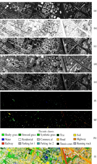
campus and the neighboring urban area. The size of the LiDAR-derived features are set to 349×1905 with the spatial resolution of 2.5m. The 15 classes of interests are: Grass Healthy, Grass Stressed, Grass Synthetic, Tree, Soil, Water, Residential, Commercial, Road, Highway, Railway, Parking Lot 1, Parking Lot 2, Tennis Court and Running Track. The “Parking Lot 1” includes parking garages at the ground level and also in elevated areas, while “Parking Lot 2” corresponded to parked vehicles. The number of training and test samples for all 15 classes are reported in Table I. It is important to note that we used exactly the same sets of training and test samples prepared for the fusion contest 2013 [7], which makes our results fully comparable with the state-of-the-art. Fig. 1.(f), (g), and (h) show the training samples, test samples, and the corresponding colorbar, respectively.
B. Algorithm Setup
In order to compare classification accuracies of different approaches, overall accuracy (OA), average accuracy (AA) and Kappa coefficient (K) have been taken into account.
In terms of the EP, the values of n used to generate the profile for different attributes are automatically given by
bαjc j = 0,1, ..., s−1. The total EP size is 2s including thinning and thickening profiles [5]. The term above was determined experimentally. The larger the α, the larger the differences between consecutive images are. The smaller the
α, the profile will concentrate in keeping few extrema, where most of the image information is usually present. Our recom-mendation is to use anαbetween2and5. In the experiments here, we used α = 3, and set s = 7. The profiles were computed considering the 4-connected connectivity rule.
RFandSVMshow a situation when RF and SVM are ap-plied todsm.EPechoratio,EPelev,EPintensity,EPdsm, and
EPsigmaz are referred to situations when an SVM with the RBF kernel (and five-fold cross-validation to tune hyperplane parameters) are performed to EPs onechoratio,elev,intensity, dsm, and sigmaz, respectively. RF EPall and SVM EPall
show situations where RF and SVM with the RBF kernel (and five-fold cross-validation to tune hyperplane parameters) are applied to the concatenation of the EPs on echoratio, elev,intensity, dsm, and sigmaz. The proposed method, CK, considers a composite kernel SVM (RBF kernel forXlidar and linear kernel forEPlidar).
C. Discussion
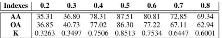
Table II investigates an optimal value for the parameter µ, which finds a trade-off between different kernels. As can be seen, the best performance is reported when µ is set to 0.5. In this way, the proposed method can define more optimal boundaries in feature space to classify different classes of interest by injecting information obtained by both LiDAR-derived features and EPs. The ignorance of the spatial infor-mation (µ= 0.2) leads to very poor performance, which prove that the EP plays an important role for the classification of the scene.
(a) (b) (c) (d) (e) (f) (g) (h) (i)
Fig. 1. (a)-(e) are the LiDAR-derived features including DSM, echo ratio, elev, intensity, and sigmaz. The figures (f)-(i) demonstrate training samples, test samples, thematic maps, and the classification map obtained by the proposed approach.
Table I demonstrates class specific accuracies for all 15 available classes followed by AA, OA, kappa, and the cor-responding CPU processing time, obtained by different ap-proaches. As can be seen the consideration of spatial informa-tion extracted by EPs (RF EPall,SVM EPall,EPintensity,
EPelev,EPdsm, andEPsigmaz) can significantly improve the classification accuracies compared to the situations where the classifiers are directly applied to the LiDAR-derived features (RF andSVM).
The proposed method demonstrates the best classification accuracy (i.e., OA, AA, and kappa) compared to the other approaches. For example, the proposed approach improved
SVM,SVM EPall, andEPdsmby almost 57.5%, 0.7%, and 19% in terms of overall accuracy, respectively. In addition, the CPU processing time of the proposed method is much less than RF EPall and SVM EPall, since it considers the linear kernel on the EPs.
Table III demonstrates the contribution of different LiDAR derived features (i.e.,dsm,intensity,elevation,echoratio, and sigmaz) on the final classification accuracy in terms of OA,
AA, kappa coefficient using the proposed composite kernel method. As can be seen, the set of features, dsm, intensity, and elevation, provides slightly the best result. The strong value of signal intensity additionally to the geometric LiDAR features is highlighted in our results, and suggests that LiDAR backscatter can compensate missing spectral optical data to a certain degree. As discusses in [8], LiDAR backscatter combines surface reflectance as well as geometry of scanned objects, and thus helps to discriminate several classes that cannot be separated in elevation or spectral data only.
IV. CONCLUSION
In this letter, we designed an effective and efficient frame-work for the classification of LiDAR point cloud derived fea-tures in terms of classification accuracy and CPU processing time. The proposed approach is based on extracting a few features such as echoratio, elevation, DSM, intensity, and sigmaz and consider them as base images for the EPs. For the classification step, the designed composite kernel SVM (RBF kernel for LiDAR-derived features and linear kernel for the concatenation of EPechoratio, EPelev, EPintensity, EPdsm, and EPsigmaz) have been taken into account. Results demon-strate that the proposed approach can effectively classify a complex urban area (more than 86% in terms of overall accuracy) composing of the 15 classes within a short CPU processing time.
V. ACKNOWLEDGMENT
The authors would like to express their appreciation to the National Center for Airborne Laser Mapping (NCALM) for providing the Houston data set. The authors would also like to appreciate the School of Electrical and Computer Engineering - UNICAMP, Brazil for providing the platform to produce extinction profile features.
REFERENCES
[1] Q. Chen, “Airborne lidar data processing and information extraction,” Photogrammetric Engineering & Remote Sensing, vol. 73, no. 2, pp. 109 – 112, 2007.
[2] M. Khodadadzadeh, J. Li, S. Prasad, and A. Plaza, “Fusion of hyperspectral and lidar remote sensing data using multiple feature learning,” IEEE Jour. Sel. Top. App. Earth Obs. Remote Sens., vol. 8, no. 6, pp. 2971– 2983, 2015.
[3] P. Ghamisi, B. H¨ofle, and X. X. Zhu, “Hyperspectral and LiDAR data fusion using extinction profiles and deep convolutional neural network,”IEEE Jour. Sel. Top. App. Earth Obs. Remote Sens., in press.
[4] J. A. Benediktsson and P. Ghamisi, Spectral-Spatial Classification of Hyperspectral Remote Sensing Images. Artech House, Boston, USA, 2015.
[5] P. Ghamisi, R. Souza, J. A. Beneiktsson, X. X. Zhu, L. Rittner, and R. Lotufo, “Extinction profiles for the classification of remote sensing data,”IEEE Trans. Geos. Remote Sens., vol. 54, no. 10, pp. 5631–5645, 2016.
TABLE I
CLASSIFICATION ACCURACY VALUES OBTAINED BY DIFFERENT APPROACHES. THE BEST ACCURAY AMONG DIFFERENT APPROACHES IS SHOWN IN BOLD TYPE FACE. THE REPORTEDCPUPROCESSING TIME(IN SECONDS)IS FOR THE CLASSIFICATION STEP.
No Name Training Test RF SVM RF EPall SVM EPall EPechoratio EPelev EPintensity EPdsm EPsigmaz CKall
1 Grass Healthy 198 1053 13.48 11.68 75.78 74.26 26.11 0 78.53 57.35 26.59 76.16 2 Grass Stressed 190 1064 16.25 0 83.55 79.51 0.18 0 78.38 40.78 38.81 80.45 3 Grass Synthetic 192 505 56.63 87.12 99.40 98.81 98.61 99.01 99.20 98.61 39.40 98.81 4 Tree 188 1056 44.03 51.79 89.67 92.89 83.80 85.13 47.25 92.32 77.36 92.99 5 Soil 186 1056 58.04 12.12 95.83 96.21 74.33 37.88 93.27 83.42 51.13 98.86 6 Water 182 143 58.04 78.32 91.60 83.91 78.32 79.02 74.82 78.32 79.02 87.41 7 Residential 196 1072 39.08 56.9 81.15 81.43 72.94 55.22 58.30 55.22 66.23 84.42 8 Commercial 191 1053 29.53 13.10 93.16 93.54 80.72 22.79 47.29 29.05 18.70 95.16 9 Road 193 1059 13.59 14.91 81.39 80.54 18.31 11.33 67.61 67.32 10.19 78.66 10 Highway 191 1036 11.29 8.30 66.98 71.42 96.33 0 97.20 61.39 62.25 74.23 11 Railway 181 1054 40.41 72.67 98.10 96.11 65.55 85.01 78.08 99.71 65.65 99.15 12 Parking Lot 1 192 1041 9.99 0 68.01 77.52 23.53 28.81 57.44 63.11 22.86 70.41 13 Parking Lot 2 184 285 15.08 12.28 69.47 82.45 43.85 35.09 64.91 49.12 56.49 79.65 14 Tennis Court 181 247 80.16 97.57 100.00 97.97 94.33 24.29 91.09 100.00 83.80 99.19 15 Running Track 187 473 75.89 27.90 97.46 97.04 0 0 94.92 74.20 45.66 97.04
Average Accuracy (AA) 37.43 36.31 86.10 86.91 57.13 28.89 75.22 70.00 49.61 87.51
Overall Accuracy (OA) 31.83 28.82 84.72 85.60 54.72 26.99 72.79 67.20 45.38 86.30
Kappa Coefficient (K) 0.2677 0.2422 0.8342 0.8445 0.5239 0.2229 0.7050 0.6440 0.4103 0.8513
CPU Processing Time 8 29 481 4692 232 180 249 237 282 119
TABLE II
THE INFLUENCE OF THEµVALUE ON CLASSIFICATION PERFORMANCE.
Indexes 0.2 0.3 0.4 0.5 0.6 0.7 0.8
AA 35.31 36.80 78.31 87.51 80.81 72.85 69.34
OA 36.85 40.73 77.02 86.30 77.22 67.11 62.94
K 0.3263 0.3497 0.7506 0.8513 0.7534 0.6447 0.6001
TABLE III
PERFORMANCE EVALUATION OF THELIDARDERIVED FEATURES. FOR THE SAKE OF SIMPLICITY,HERE,int,ele,ech,ANDsigREPRESENT
intensity,elevation,echoratio,ANDsigmaz,RESPECTIVELY.
Indexes CKdsm,int CKdsm,int,ele CKdsm,int,ech CKdsm,int,sig
AA 84.54 87.34 82.77 83.27
OA 82.55 85.93 80.63 81.88
K 0.8106 0.8473 0.7917 0.8034
[6] P. Ghamisi, R. Souza, J. A. Benediktsson, L. Rittner, R. Lotufo, and X. X. Zhu, “Hyperspectral data classi-fication using extended extinction profiles,” IEEE Geos. Remote Sens. Let., vol. 13, no. 11, pp. 1641–1645, 2016. [7] C. Debes, A. Merentitis, R. Heremans, J. Hahn, N. Frangiadakis, T. van Kasteren, W. Liao, R. Bellens, A. Pizurica, S. Gautama, W. Philips, S. Prasad, Q. Du, and F. Pacifici, “Hyperspectral and lidar data fusion: Outcome of the 2013 grss data fusion contest,” IEEE Jour. Selec. Top. App. Earth Obs. Remote Sens., vol. 7, no. 6, pp. 2405–2418, June 2014.
[8] B. H¨ofle, M. Hollaus, and J. Hagenauer, “Urban vege-tation detection using radiometrically calibrated small-footprint full-waveform airborne lidar data,”ISPRS Jour. Photo. Remote Sens., vol. 67, pp. 134–147, 2012. [9] N. Pfeifer, G. Mandlburger, J. Otepka, and W. Karel,
“{OPALS} a framework for airborne laser scanning data analysis,” Computers, Environment and Urban Systems, vol. 45, pp. 125 – 136, 2014.
[10] B. H¨ofle and N. Pfeifer, “Correction of laser scanning in-tensity data: Data and model-driven approaches,”ISPRS Jour. Photo. Remote Sens., vol. 62, no. 6, pp. 415 – 433, 2007.
[11] M. Hollaus, C. Aubrecht, B. Hfle, K. Steinnocher, and W. Wagner, “Roughness mapping on various vertical scales based on full-waveform airborne laser scanning data,” Remote Sensing, vol. 3, no. 3, p. 503, 2011. [12] P. Ghamisi, M. Dalla Mura, and J. A. Benediktsson, “A
survey on spectral–spatial classification techniques based on attribute profiles,” IEEE Trans. Geos. Remote Sens., vol. 53, no. 5, pp. 2335–2353, 2015.
[13] E. Carlinet and T. Geraud, “A comparative review of component tree computation algorithms,” IEEE Trans. Image Proc., vol. 23, no. 9, pp. 3885–3895, Sept 2014. [14] R. Souza, L. Rittner, R. Lotufo, and R. Machado, “An
array-based node-oriented max-tree representation,” in ICIP’15, Sept 2015, pp. 3620–3624.
[15] T. M. Cover, “Geometrical and statistical properties of systems of linear inequalities with application in pattern recognition,” IEEE Trans. Electron. Comp., vol. EC-14, pp. 326–334, 1965.
[16] B. Scholkopf and A. J. Smola, Learning with Kernels. MIT Press, 2002.
[17] B. Schlkopf and A. Smola, Learning With Kernels-Support Vector Machines, Regularization, Optimization and Beyond. Cambridge, MA: MIT Press, 2002. [18] C. J. C. Burges, “A tutorial on support vector machines
for pattern recognition,” Data Mining and Knowledge Discovery, vol. 2, no. 2, pp. 121–167, 1998.
[19] G. Camps-Valls, L. Gomez-Chova, J. Munoz-Mari, J. Vila-Frances, and J. Calpe-Maravilla, “Composite ker-nels for hyperspectral image classfication,” IEEE Geos. Remote Sens. Lett., vol. 3, no. 1, pp. 93–97, 2006.