Lecture 6: Discovering Domain Entities

5. Discovering Domain Entities

• Lecture 2 briefly characterised, informally and also a bit more

formally, what we mean by a domain.

• Lecture 3 informally and systematically characterised the four

categories of entities: parts, actions, events and behaviours.

• Lectures 4–5 more-or-less “repeated” Sect. 3’s material but by now

giving more terse narratives (that is, informal descriptions) and, for the fist time, also formalisations.

• Lectures 4–5 did not hint at how one discovers domain parts (i.e.,

their types), actions, events and behaviours.

• In this section we try unravel a set of techniques and tools —

5.1. Preliminaries

• Before we present the discoverers and analysers we need establish

some concepts. These are:

– Part Signatures Slides 223–224

– Domain Indices Slides 225–226

– Inherited Part Signatures Slides 227–227

– Domain Signatures Slides 228–231

5.1.1. Part Signatures

• Let us consider a part p : P.

• Let p : P, by definition, be the principal part of a domain. – Now we need to identify

∗ (i) the type, P, of that part;

∗ (ii) the types, S₁, . . . , Sm, of its proper sub-parts (if p is composite);

∗ (iii) the type, PI, of its unique identifier;

∗ (iv) the possible types, MI₁, . . . , MIn, of its mereology; and

∗ (v) the types, A₁, . . . , Ao, of its attributes.

• We shall name that cluster of type identifications – the part signature.

• We refer to P as identifying the part signature. • Each of the S (for i : {1..m}) identifies sub-parts

Example 41 (Net Domain and Sub-domain Part Signatures)

The part signature of the hubs and the links are here chosen to be those of

• (i) N, • (ii) Hs, • (ii) Ls and

• Net name, Net owner, etc.

The part signatures Hs and Ls are • (ii) Hs = H-set, H

• (iii,iv) HI, LI-set

• (v) Hub Nm, Location, HΣ, HΩ, ...

• (ii) Ls = L-set, L

5.1.2. Domain Indices

• By a domain index we mean a list of part type names that identify

a sequence of part signatures.

• More specifically

– The domain ∆ has index h∆i.

– The sub-domains of ∆, with part types A, B, ..., C, has indices

h∆,Ai, h∆,Bi, . . . , h∆,Ci.

– The sub-domains of sub-domain with index ℓ and with part

Example 42 (Indices of a Road Pricing Domain) We refer to

the the Road-pricing Transport Domain, cf. Example 36 on page 184.

The sub-domain indices of the road-pricing transport domain, ∆, are:

• h∆i, • h∆,Ni, • h∆,Fi, • h∆,Mi, • h∆,N,Vsi, • h∆,N,Lsi, • h∆,N,Hi, • h∆,N,Li and • h∆,F,Vi. •

5.1.3. Inherited Domain Signatures

• Let h∆,A,B,C,Di be some domain index.

• Then

– h∆,A,B,Ci – h∆,A,Bi – h∆,Ai – h∆i

5.1.4.

• By the domain category of the domain indexed by ℓ_bhDi we shall

mean

– the domain signature of D,

and the

– action,

– event and

– behaviour

definitions whose signatures involves

– just the types given in the domain signature of D or

Example 43 (The Road-pricing Domain Category) The road-pricing domain category consist of

• the types N, F and M,

• the create Net create Fleet and create M actions, and

• corresponding Net, Fleet and M behaviours

• By a sub-domain category, of index ℓ, we shall mean

– the sub-domain types of the sub-domain designated by index ℓ,

and the

– actions,

– events and

– behaviours

whose signatures involves just the types

– of the ℓ indexed sub-domain

– or of any prefix of ℓ indexed sub-domain

Example 44 (A Hub Category of a Road-pricing Transport Domain)

The ancestor sub-domain types of the hub sub-domain are: HS, N

and ∆.

• The hub category thus includes

– the part (etc.) types H, HI, ...,

– the insert Hub and the delete Hub actions,

– perhaps some saturated hub (and/or other) event(s),

– but probably no hub behaviour as it would involve at least the

type LI which is not in an ancestor sub-domain of the Hub

sub-domain.

5.1.5. Simple and Compound Indexes

• By a simple index we mean a domain or a sub-domain index.

• By a compound index we mean a set of two or more distinct indices

of a domain ∆.

• Compound indices, c_idx : {ℓ_i, ℓ_j, . . . , ℓ_k}, designate parts, actions,

events and behaviours each of whose types and signatures involve

types defined by all of the simple indexes of c_idx.

Example 45 (Compound Indices of the Road-pricing System)

We show just one compound index:

• {h∆,N,HS,Hi,h∆,N,LS,Li}.

5.1.6. Simple and Compound Domain Categories

• By a simple domain category we shall mean any ℓ-indexed

[sub-]domain category.

• By the compound domain category of compound index

c_idx : {ℓ_i, ℓ_j, . . . , ℓ_k}, we shall mean

– the set of types, actions, events and behaviours

– as induced by compound index c_idx, that is,

– parts, actions, events and behaviours

– each of whose types and signatures involve types defined by all of

Example 46 (The Compound Domain Category of Hubs and Links)

The compound domain category designated by

{h∆,N,HS,Hi,h∆,N,LS,Li} includes:

type

HIs = HI-set

axiom ∀ his:HIs•card his=2

LIs = LI-set

HΣ = (LI×LI)-set

LΣ = (HI×HI)-set

HΩ = HΣ-set LΩ = LΣ-set value mereo L: L → HIs, mereo H: H → LIs attr HΣ: H → HΣ attr LΣ: L → LΣ attr HΩ: H → HΩ attr LΩ: L → LΩ axiom ∀ h:H•attr HΣ(h)⊆attr HΩ(h) ∀ l:L•attr LΣ(l)⊆attr LΩ(l) •

5.1.7. Examples

• We repeat some examples, but now “formalised”.

Example 47 (The Root Domain Category) We start at the root, ∆, of the Road Pricing Domain. See Fig. 13.

∆

< >

∆

Figure 13: The h∆i Root

N F M

∆ ∆

∆

New indices: {< ,N>,< ,F>,< ,M>}∆

When observing the very essence of the road pricing domain “at the

h∆i level” one observes:

type N, F, M value obs N: ∆ → N obs F: ∆ → F obs M: ∆ → M attr ...: ∆ → ...

where ... stands for types of road pricing domain attributes.

Example 48 (The Net Domain Category) We then proceed to

explore the domain at index h∆,Ni. See Fig. 15.

F

M

Hs

Ls

∆

∆

∆

N

New indices: {< ,N,Hs>,< ,N,Ls>}

When observing the very essence of the Net domain, “at the h∆, Ni

level” one observes:

type Hs = H-set Ls = L-set H L ... value obs Hs: N → Hs obs Ls: N → Ls attr Hs: Hs → ... attr Ls: Ls → ...

where ... stand for attributes of the Hs and the Ls parts of N.

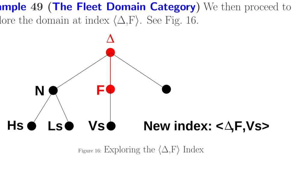
Example 49 (The Fleet Domain Category) We then proceed to

explore the domain at index h∆,Fi. See Fig. 16.

N

Hs

Ls

Vs

New index: < ,F,Vs>

∆

∆

F

When observing the very essence of the Fleet domain, “at the h∆, Fi

level” one observes:

type Vs = V-set V ... value obs Vs: F → Vs attr ... Vs → ...

where ... stand for attributes that we may wish to associate with

Fleets of vehicles.

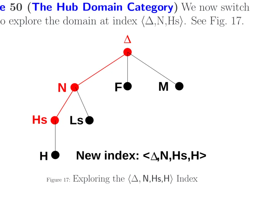
Example 50 (The Hub Domain Category) We now switch

“back” to explore the domain at index h∆,N,Hsi. See Fig. 17.

F

M

Ls

H

New index: < ,N,Hs,H>

∆

∆

N

Hs

When observing the very essence of the Fleet domain, “at the

h∆, N,Hs,Hi level” one observes:

type HI ... value uid HI: H → HI attr ...: H → ...

where ... stand for LOCation, etc.

Example 51 (The Link Domain Category) Next we explore the link domain. See Fig. 18.

N F M

Hs Ls

H H

New index: < ,N,Ls,L>∆

∆

When observing the very essence of the Fleet domain, “at the

h∆, N,Ls,Li level” one observes:

type LI ... value uid LI: L → LI attr ...: L → ...

where ... stand for LOCation, LENgth, etc.

Example 52 (The Compound Hub and Link Domain Category)

We next explore a compound domain. See Fig. 19.

F

M

Exploring composite index:

∆

N

Hs

Ls

H

L

{< ,N,Hs,H>,< ,N,Ls,L>}

∆

∆

When observing the very essence of the Fleet domain, at the {h∆, N,Hs,Hi,h∆, N,Ls,Li} level one observes:

type

HΣ = (LI×LI)-set, HΩ = HΣ-set, LΣ = (HI×HI)-set, LΩ = LΣ-set value

attr HΣ: H → HΣ, attr HΩ: H → HΩ attr LΣ: L → LΣ, attr LΩ: L → LΩ

mereo L: L → HI-set axiom ∀ l:L:card mereo L(l)=2 mereo H: H → LI-set (= LI-set)

remove H: HI → N →∼ N insert L: L → N →∼ N remove L: LI → N →∼ N ... axiom ∀ hσ:HΣ ..., ∀ hω:HΩ ... ∀ lσ:HΣ ..., ∀ lω:HΩ ...

5.1.8. Discussion

• The previous examples (47–52), especially the last one (52),

– illustrates the complexity of a domain category;

– from just observing sub-part types and attributes (as in

Examples 47–49),

– Example 52 observations grow to intricate mereologies etcetera.

• The ‘discoverers’ that we shall propose

– aim at structuring the discovery process by focusing, in turn, on

∗ part sorts,

∗ concrete part types,

∗ unique identifier types of parts, ∗ part mereology,

∗ part attributes, ∗ action signatures, ∗ event signatures, ∗ etc.

5.2. Proposed Type and Signature ‘Discoverers’ • By a ‘domain discoverer’ we shall understand

– a tool and a set of principles and techniques – for using this tool

– in the discovery of the entities of a domain.

• In this section we shall put forward a set of type and signature discoverers. – Each discoverer is indexed by a simple or a compound domain index. – And each discoverer is dedicated to some aspect of some entities.

• Together the proposed discoverers should cover the most salient aspects of domains.

• Our presentation of type and signature discoverer does not claim to help analyse “all” of a domain.

• We need formally define what an index is. type

Index = Smpl Idx | Cmpd Idx

Smpl Idx = {| h∆i_bidx | idx:Type Name∗ |} Cmpd Idx′ = Smpl Idx-set

Cmpd Idx = {| sis:Cmpd Idx′

• wf Cmpd Idx(sis) |}

value

wf Cmpd Idx: Cmpd Idx′

→ Bool wf Cmpd Idx(sis) ≡ ∀ si,si′

:Smpl Idx • {si,si′}⊆sis ∧ si6=si′

DISCOVERER KIN D: Index → Text DISCOVER KIN D(ℓ_bhti) as text

pre: ℓ_bhti is a valid index beginning with ∆ post: text is some, in our case, RSL _text

– where DISCOVERER KIN D is any of the several different “kinds” of domain forms:

[90 (Slide 255)] PART SORTS,

[91 (Slide 257)] HAS A CONCRETE TYPE, [92 (Slide 260)] PART TYPES,

[93 (Slide 264)] UNIQUE ID, [96 (Slide 265)] MEREOLOGY, [98 (Slide 267)] ATTRIBUTES,

[100 (Slide 275)] ACTION SIGNATURES, [101 (Slide 276)] EVENT SIGNATURES and [103 (Slide 280)] BEHAVIOUR SIGNATURES.

• In a domain analysis (i.e., discovery) the domain description emerges “bit-by-bit”.

– Initially types are discovered and hence texts which define ∗ unique identifier types and functions,

• The two most important aspects of an algebra are those of

– its parts and

– its operations.

• Rather than identifying, that is, discovering or analysing individual

parts

– we focus on discovering their types —

– initially by defining these as sorts.

• And rather than focusing on defining what the operations achieve

– we concentrate on the signature,

• It (therefore) seems wise to start with the discovery of parts, and hence of their types.

– Part types are present in the signatures of all actions, events and

behaviours.

– When observing part types we also observe a variety of part type

analysers:

∗ possible unique identities of parts,

∗ the possible mereologies of composite parts, and

5.2.1.1. Domain Part Sorts and Their Observers

• Initially we “discover” parts —

– by deciding upon their types,

– in the form, first of sorts,

5.2.1.1.1. A Domain Sort Discoverer

90. A part type discoverer applies to a simply indexed domain, index,

and yields

(a) a set of type names

(b) each paired with a part (sort) observer.

value

90. PART SORTS: Index →∼ Text

90. PART SORTS(ℓ_bhTi):

90(a). tns:{T₁,T₂,...,Tm}:TN-set ×

Example 53 (Some Part Sort Discoveries) We apply a concrete version of the above sort discoverer to the road-pricing transport domain ∆:

PART SORTS_(h∆i):

type N, F, M value obs N: ∆ → N obs F: ∆ → F obs M: ∆ → M

PART SORTS_(h∆,Ni):

type Hs, Ls value

obs Hs: N → Hs obs Ls: N → Ls

PART SORTS(h∆,Fi):

type Vs value

obs Cs: F → Vs

5.2.1.2. Domain Part Types and Their Observers

5.2.1.2.1. Do a Sort Have a Concrete Type ?

• Sometimes we find it expedient

– to endow a “discovered” sort with a concrete type expression,

that is,

– “turn” a sort definition into a concrete type definition.

91. Thus we introduce the “discoverer”:

91 HAS A CONCRETE TYPE: Index → Bool

Example 54 (Some Type Definition Discoveries) We exemplify two true expressions:

HAS A CONCRETE TYPE(h∆,N,Hsi)

HAS A CONCRETE TYPE_(h∆,N,Lsi)

∼ HAS A CONCRETE TYPE(h∆,N,Hs,Hi)

∼ HAS A CONCRETE TYPE(h∆,N,Ls,Li)

5.2.1.2.2. A Domain Part Type Observer

• The PART TYPES(ℓ_bhti) invocation yields one or more sort definitions of part types together with their observer functions.

– The domain analyser can decide that some parts can be

immediately analysed into concrete types.

– Thus, together with yielding a type name, the PART TYPES

can be expected to yield also a type definition, that is, a type expression (paired with the type name).

– Not all type expressions make sense.

92. The PART TYPES discoverer applies to a composite type, t, and yields

(a) a type definition, T = TE,

(b) together with the sort and/or type definitions of so far undefined

type names of TE.

(c) The PART TYPES discoverer is not defined if the designated

sort is judged to not warrant a concrete type definition.

92. PART TYPES_{: Index →}∼ _Text

92. PART TYPES(ℓ_bhti):

92(a). type t = te,

92(b). T₁ or T₁ = TE₁ 92(b). T₂ or T₂ = TE₂ 92(b). ...

Example 55 (Some Part Type Discoveries) We exemplify two discoveries:

PART TYPES_{(h∆,N,Hsi):}

type H

Hs = H-set

PART TYPES(h∆,N,Lsi):

type L

Ls = L-set

PART TYPES_(h∆,Fi):

type V

5.2.1.2.3. Concrete Part Types

• In Example 55 on the preceding page we illustrated one kind of concrete part type: sets.

• Practice shows that sorts often can be analysed into sets. • Other analyses of part sorts are

– Cartesians, – list, and – simple maps: 90(b). te: tn1 × tn2 × ... × tnm 90(b). te: tn∗ 90(b). te: Token →m tn • where

5.2.1.3. Part Type Analysers

• There are three kinds of analysers:

– unique identity analysers,

– mereology analysers and

5.2.1.3.1. Unique Identity Analysers

• We associate with every part type T, a unique identity type TI.

93. So, for every part type T we postulate a unique identity analyser function uid TI. value

93. UNIQUE ID: Index → Text 93. UNIQUE ID₍ℓ_bhTi):

93. type 93. TI 93. value

5.2.1.3.2. Mereology Analysers

• Given a part, p, of type T, the mereology, MEREOLOGY_{, of that part}

– is the set of all the unique identifiers

of the other parts to which part p is partship-related – as “revealed” by the mereo TIi functions applied to p.

94. Let types T₁, T₂, . . . , T_n be the types of all parts of a domain.

95. Let types TI₁, TI₂, . . . , TI_n22, be the types of the unique identifiers of all parts of that domain.

96. The mereology analyser MEREOLOGY is a generic function which applies to an index and yields the set of

(a) zero, (b) one or

type

94. T = T₁ | T₂ | ... | Tn

95. T_idx = TI₁ | TI₂ | ... | TI_n

96. MEREOLOGY: Index → Text

96. MEREOLOGY({ℓ_ibhT_ji,...,ℓ_kbhT_li}):

96(a). either: {}

96(b). or: mereo TIx: T → (TIx|TIx-set)

96(c). or: { mereo TIx: T → (TIx|TIx-set),

96(c). mereo TI_y: T → (TI_y|TI_y-set),

96(c). ...,

96(c). mereo TI_z: T → (TI_z|TI_z-set) }

• where none of TIx, TIy, . . . , TIz are equal to TI and each is some

5.2.1.3.3. General Attribute Analysers

• A general attribute analyser analyses parts beyond their unique

identities and possible mereologies.

97. Part attributes have names. We consider these names to also abstractly name the corresponding attribute types, that is, the names function both as attribute names and sort names. Finally we allow attributes of two or more otherwise distinct part types to be the same.

98. ATTRIBUTES applies to parts of any part type t and yields

99. the set of attribute observer functions attr at, one for each

type

97. AT = AT₁ | AT₂ | ... | AT_n

value

98. ATTRIBUTES_{: Index → Text}

98. ATTRIBUTES(ℓ_bhTi): 99. type 99. AT₁, AT₂, ..., AT_m 99. value 99. attr AT₁: T → AT₁ 99. attr AT₂: T → AT₂ 99. ..., 99. attr AT_m: T → AT_m, m≤n

Example 56 (Example Part Attributes) We exemplify attributes of composite and of atomic parts:

ATTRIBUTES(h∆i):

type

Domain Name, ...

value

attr Name: ∆ → Domain Name

...

• where

– Domain Name could include State Roads or Rail Net.

ATTRIBUTES(h∆,Ni):

type

Sub Domain Location, Sub Domain Owner, Kms, ...

value

attr Location: N → Sub Domain Location

attr Owner: N → Sub−Domain Owner

attr Length: N → Kms

...

• where

– Sub Domain Location could include Denmark,

– Sub Domain Owner could include The Danish Road Directorate23, respectively BaneDanmark24,

ATTRIBUTES_{(h∆,N,Hs,Li):}

type

LOC, LEN, ...

value

attr LOC: L → LOC attr LEN: L → LEN

... ATTRIBUTES_{({h∆,N,Hs,Li.h∆,N,Hs,Hi}):} type LΣ = HI-set, LΩ − LΣ-set HΣ = LI-set, HΩ − HΣ-set value attr LΣ: L → LΣ attr LΩ: L → LΩ attr HΣ: H → HΣ attr HΩ: H → HΩ • where

– LOC might reveal some Bezier curve25 representation of the possibly curved three dimensional location of the link in question,

– LEN might designate length in meters,

⋆ Attribute Sort Exploration ⋆

• Once the attribute sorts of a part type have been determined

– there remains to be “discovered” the concrete types of these

sorts.

– We omit treatment of this point in the present version of these

5.2.2. Discovering Action Signatures

5.2.2.1. General

• We really should discover actions, but actually analyse function

definitions.

• And we focus, in these lectures, on just “discovering” the function

signatures of these actions.

• By a function signature, to repeat, we understand

– a functions name, say fct, and

– a function type expression (te), say dte→rte∼ where

∗ dte defines the type of the function’s definition set

5.2.2.2. Function Signatures Usually Depend on Compound Domains

• We use the term ‘functions’ to cover actions, events and behaviours.

• We shall in general find that the signatures of actions, events and

behaviours depend on types of more than one domain.

– Hence the schematic index set {ℓ_1bht₁i,ℓ_2bht₂i,...,ℓ_nbhtni}

5.2.2.3. The ACTION SIGNATURES Discoverer

100. The ACTION SIGNATURES meta-function applies to an index set and yields (a) a set of action signatures each consisting of an action name and a pair of

definition set and range type expressions where

(b) the type names that occur in these type expressions are defined by in the domains indexed by the index set.

100 ACTION SIGNATURES_{: Index →}∼ _Text

100 ACTION SIGNATURES_({ℓ_1bhT1i,ℓ2bhT2i,...,ℓnbhTni}):

100(a) act fcti: tei_d ∼ → teir, 100(a) act fctj: tej_d ∼ → tejr, 100(a) ... , 100(a) act fctk: tek_d ∼ → tekr 100(b) where:

• Events are from the point of view of signatures very much like actions.

101. The EVENT SIGNATURES _{meta-function applies to an index set and yields}

(a) a set of action signatures each consisting of an action name and a pair of definition set and range type expressions where

(b) the type names that occur in these type expressions are defined either in the domains indexed by the index set or by the environment (i.e., “outside” the domain ∆).

101 EVENT SIGNATURES_{: Index →}∼ _Text 101 EVENT SIGNATURES_({ℓ_1bhT₁i,ℓ_2bhT₂i,...,ℓ_nbhTni}): 101(a) evt fct_i: te_id →∼ te_ir, 101(a) evt fct_j: te_jd →∼ te_jr, 101(a) ... , 101(a) evt fct_k: te_kd →∼ te_kr 101(b) where: 101(b) type names of te_(i|j|...|k)

d and te(i|j|...|k)r are type names

101(b) defined by the indices which are prefixes of ℓ_mbht_mi

101(b) and where tm is in some signature act fct_i|j|...|k or may

• We choose, in these lectures, to model behaviours in CSP26_.

• This means that we model (synchronisation and) communication between

behaviours by means of messages m of type M, CSP _{channels (channel ch:M)}

and CSP

output: ch!e [offer to deliver value of expression e on channel ch], and input: ch? [offer to accept a value on channel ch].

• We allow for the declaration of single channels as well as of one, two, ..., n

dimensional arrays of channels with indexes ranging over channel index types type Idx, CIdx, RIdx . . .:

channel ch:M, { ch v[vi]:M′|vi:Idx }, { ch m[ci,ri]:M′′|ci:CIdx,ri:RIdx }, . . . etcetera.

• A behaviour usually involves two or more distinct sub-domains.

Example 57 (The Involved Subdomains of a Vehicle Behaviour)

Let us illustrate that behaviours usually involve two or more distinct sub-domains.

• A vehicle behaviour, for example, involves

– the vehicle subdomain,

– the hub subdomain (as vehicles pass through hubs),

– the link subdomain (as vehicles pass along links) and,

– for the road pricing system, also the monitor subdomain.

102. The BEHAVIOUR SIGNATURES _{is a meta function.}

103. It applies to a set of indices and results in a text, 104. The text contains

(a) a set of zero, one or more message types,

(b) a set of zero, one or more channel index types, (c) a set of zero, one or more channel declarations,

(d) a set of one or more process signatures with each signature containing a behaviour name, an argument type expression, a

result type expression, usually just Unit, and

(e) an input/output clause which refers to channels over which the signatured behaviour may interact with its environment.

103. BEHAVIOUR SIGNATURES_{: Index →}∼ _Text

103. BEHAVIOUR SIGNATURES({ℓ_1bhT₁i,ℓ_2bhT₂i,...,ℓ_nbhT_ni}):

104(a). type M = M₁ | M ₂| ... | Mm, m≥0

104(b). I = I₁ | I₂ | ... | In, n≥0

104(c). channel ch,vch[ i ],{vch[ i ]:M|i:Ia},{mch[ j,k ]:M|j:Ib,k:Ic},...

104(d). value

104(d). bhv₁: ate₁ → inout₁ rte₁, 104(d). bhv₂: ate₂ → inout₂ rte₂, 104(d). ... ,

104(d). bhvm: atem → inoutm rtem,

104(d). where type expressions ateii and rtei for all i involve at least two

104(d). types t′_i and t′′_j of respective indexes ℓ_ibhtii and ℓjbhtji

104(e). where inout_i: in k | out k | in,out k

Example 58 (A Vehicle Behaviour Signature Discovery) We refer, for example, to Examples 36 (Slides 184–198) and 40 (Slides 215–219).

let ih=h∆.N.LS,Hi,il=h∆.N.HS,Li,iv=h∆,F,Vi,im=h∆,Monitori in

BEHAVIOUR SIGNATURES_{({iv,ih,iv,im}) as text}

let n:N, hs=obs HS(n), ls=obs LS(n), vs=obs F(PART SORTS)(h∆i) in where text:

type

VL Msg, VH Msg, VM Msg channel

62(a). {vh ch[ attr VI(v),attr HI(h) ]|v:V,h:H•v ∈ vd∧h ∈ hs}:VH Msg

62(b). {vl ch[ attr VI(v),attr LI(h) ]|v:V,l:L•v ∈ vs∧h ∈ ls}:VL Msg

62(c). m ch:VM Msg value

64. vehicle: VI → V → VP →

83. out,in {vl ch[ vi,li ]|li:LI•li ∈ xtr LIs(ls)}

83. {vh ch[ vi,hi ]|hi:HI•hi ∈ xtr HIs(hs)} out m ch,... Unit

5.3. What Does Application Mean ?

• Now what does it actually mean “to apply” a discover function ?

• We repeat our list of discoverers.

[90 (Slide 255)] PART SORTS,

[91 (Slide 257)] HAS A CONCRETE TYPE_,

[92 (Slide 260)] PART TYPES_,

[93 (Slide 264)] UNIQUE ID_,

[96 (Slide 265)] MEREOLOGY_,

[98 (Slide 267)] ATTRIBUTES,

[100 (Slide 275)] ACTION SIGNATURES, [101 (Slide 276)] EVENT SIGNATURES _and

• The first “formal” domain inquiry is that of PART SORTS(h∆i).

– We refer to Item 90 on page 255, for example as captured by the

formulas, Items 90–90(b) (Slide 285).

• For the domain engineer to ‘issue’ one of the ‘discovery commands’

means that that person has

– (i) prepared his mind to study the domain and is open to

impressions,

– (ii) decided which DISCOVERER KIN D to focus on, and

– (iii) studied the “rules of engagement” of that command, that is

∗ which pre-requisite discoverers must first have been applied,

∗ with which index, that is, in which context the command

5.3.1. PART SORTS

• Let us review the PART SORTS discoverer:

value

90. PART SORTS: Index →∼ Text

90. PART SORTS₍ℓ_bhTi):

90(a). tns:{T₁,T₂,...,Tm}:TN-set ×

90(b). { obs T_j: T → T_j | T_j:tns}

• The domain analyser has decided to “position” the search at

domain index ℓ_bhTi

– where T = ∆ if ℓ = hi and

• From Item 90(a) the domain analyser is guided (i.e., advised) to

analyse the domain “at position ℓ_bhTi:

– is the domain type T a type of one or more subpart types ?

∗ If so then decide which they are, that is: T₁,T₂,...,Tm,

that is, the “generation” of the text type T₁,T₂,...,Tm,

∗ if not then tns={} and no text is “generated”.

• Item 90(b), and given the domain analyser’s resolution of

Item 90(a), then directs

– the “generation” of m observers obs T_j: T → T_j

5.3.2. HAS A CONCRETE TYPE

• Let us review the HAS A CONCRETE TYPE analyser:

91 HAS A CONCRETE TYPE: Index → Bool

91 HAS A CONCRETE TYPE(ℓ_bhTi):true|false

• Item 91 directs the domain analyser to decide

– whether the domain type T at “position” ℓ_bhti

– should be given a concrete type definition.

• It is a decision sˆolely at the discretion of the domain analyser

– whether domain type T should be given a concrete type

definition,

5.3.3.

• Let us review the PART TYPES analyser:

92. PART TYPES: Index →∼ Text

92. PART TYPES(ℓ_bhti):

92(a). type T = TE,

92(b). T₁ or T₁ = TE₁

92(b). T₂ or T₂ = TE₂

92(b). ...

92(b). T_n or T_n = TE_n

• The domain analyser has decided to “position” the search at

domain index ℓ_bhTi

– where T = ∆ if ℓ = hi and

– where T is some “previously discovered part type.

• From Item 92 the domain analyser is guided (i.e., advised) to

analyse the domain “at position ℓ_bhTi:

– can an abstract, yet concrete type definion be given for T ?

– If so then decide which it should be, that is, should it be an

atomic type

∗ a number type, Intg, Rat, Real,

∗ a Boolean type, Bool, or

– or should it be a composite type

∗ either a set type: TE: Ts-set of te: Ts-infset, ∗ or a Cartesian type: TE: T1×T2×...Tm,

∗ or a list type: TE: T⋆_ℓ or te: Tω_ℓ

∗ or a map type: TE: Td →m Tt ?

• In either case the text – type T = TE, – T₁ or T₁=TE₁, – T₂ or T₁=TE₂, – ..., – Tn or Tn=TEn is generated

• where TE (TEx) is a type expression whose

5.3.4. UNIQUE ID

• Let us review the UNIQUE ID _analyser:

value

93. UNIQUE ID_{: Index → Text}

93.a UNIQUE ID(ℓ_bhTi):

93.b type 93.c TI 93.d value

93.e uid TI: T → TI

• Item 93.a inquires as to the

• Line 93.b type name

• Line 93.c of the inquired part type’s unique identifiers

• Line 93.d and the function signature value

• Etcetera, etcetera.

5.4. Discussion

• We have presented a set of discoverers:

[90 (Slide 255)] PART SORTS,

[91 (Slide 257)] HAS A CONCRETE TYPE_,

[92 (Slide 260)] PART TYPES,

[93 (Slide 264)] UNIQUE ID,

[96 (Slide 265)] MEREOLOGY_,

[98 (Slide 267)] ATTRIBUTES,

[100 (Slide 275)] ACTION SIGNATURES,

[101 (Slide 276)] EVENT SIGNATURES and

• There is much more to be said:

– About a meta-state component in which is kept the “text” so far

generated.

– A component from which one can see which indices and hence

which type names have so far been “generated”,

– and on the basis of which one can perform tests of

well-formedness of generated text,