GEOLOGICA ULTRAIECTINA
Mededelingen van de
Faculteit Aardwetenschappen
Universiteit Utrecht
No. 127GEODYNAMIC EVOLUTION
AND
MANTLE STRUCTURE
MARC DE JONGE
27-012
CIP-GEGEVENS KONINKLIJKE BIBLIOTHEEK, DEN HAAG Jonge, Marc Rene de
Geodynamic evolution and mantle structure / Marc Rene de Jonge.
- Utrecht : Faculteit Aardwetenschappen, Universiteit Utrecht. - (Geologica Ultraiectina, ISSN 0072-1026 ; no. 127)
Proefschrift Universiteit Utrecht. - Met lit. opg. Met samenvatting in het Nederlands.
ISBN 90-71577-81-3
Trefw.: geodynamica ; Middellandse Zee-gebied / tomografie ; Middellandse Zee-gebied.
GEODYNAMIC EVOLUTION AND
MANTLE STRUCTURE
Geodynamische ontwikkeling en mantelstructuur
(met een samenvatting in het Nederlands)
PROEFSCHRIFT
TER VERKRIJGING VAN DE GRAAD VAN DOCTOR
AAN DE UNIVERSITEIT UTRECHT,
OP GEZAG VAN DE RECTOR MAGNIFICUS
PROF. DR. J. A. VAN GINKEL, INGEVOLGE HET BESLUIT
VAN HET COLLEGE VAN DEKANEN IN HET OPENBAAR
TE VERDEDIGEN OP
WOENSDAG 13 SEPTEMBER 1995
OM HALF DRIE 'S MIDDAGS
DOOR
MARC RENE DE JONGE
PROMOTOR: PROF. DR. M.
J.
R. WORTEL
COPROMOTOR: DR. W. SPAKMAN
The research in this study was carried out at the Department of Geophysics of the Institute of Earth Sciences, Utrecht University, Budapestlaan 4, 3584 DC Utrecht, The Netherlands. It was funded by NWO/AWON (Netherlands Organisation for Scientific Research, Earth Sciences branch) as project 751-354-019.
The tomographic inversions described in chapter 4 were calculated at the NCF (National Computer Facilities) in Amsterdam and were funded with grant SC-245.
The following publications have resulted from this study:
M. R. de Jonge and M. J. R. Wortel, The thermal structure of the Mediterranean upper mantle; a forward modelling approach, Terra Nova, 2, 609-616, 1990.
M. R. de Jonge, M. J. R. Wortel, and W. Spakman, From tectonic evolution to upper mantle model: an application to the Alpine-Mediterranean region, Tectonophysics, 223, 53-65, 1993.
M. R. de longe, M. J. R. Wartel, and W. Spakman, Regional scale tectonic evolution and the seismic velocity structure of the lithosphere and upper mantle: the Mediterranean region.
J. Geophys. Res., 99, 12091-12108, 1994. (chapter 3)
M. R. de Jonge, W. Spakman, and M. J. R. Wortel, Geodynamic evolution of the Alpine Mediterranean region: a tomographic analysis, J. Geophys. Res., <submitted>, 1995. (chapter 4)
After all, it is possible I may be mistaken; and it is but a little copper and glass, perhaps, that I take for gold and diamonds. I know how very liable we are to delusion in what relates to ourselves, and also how much the judgements of our friends are to be suspected when given in our favour. But I shall endeavour in this discourse to describe the paths I have followed ...
Rene Descartes, Discourse on the method of rightly conducting the reason and seeking truth in the sciences, 1637
- Contents - 7
Contents:
Introduction 9
Chapter 1, Mesozoic and Cenozoic tectonic evolution of the
Alpine-Mediterranean region 14
1.1 Introduction 15
1.2 Tectonic reconstructions 16
Chapter 2, Thermal modelling of tectonic processes 27
2.1 Initial thermal structure 28 2.2 Determining a kinematic model from a tectonic reconstruction 33 Convergent plate boundaries 34
Intra-plate extension 36
2.3 Calculating the thermal development from the initial structure and the
kinematic model 37
2.4 Determining thermally controlled quantities 41
Basement heat flow density 41
Basin topography 42
P-wave velocity structure 43
Appendix 1, The temperature distribution of the upper mantle 51 Chapter 3, Forward models for the seismic velocity structure
of the Alpine-Mediterranean region 57
3.1 Introduction 58
3.2 Forward Modelling Procedure 59 Stage 1: constructing a displacement field from a tectonic reconstruction 60
Convergent plate boundaries (61 ) Intra-plate extension (63)
Stage 2: thermal model 64
Initially oceanic regions (65) Initially continental regions (65) Initial mantle structure (65)
Thermal development of initial structures (65)
Time-dependent three-dimensional temperature structure (66)
Stage 3: from model temperature to geophysically observable quantities 66
Seismic velocity perturbations (66)
Thermal subsidence and heat flow density (67)
3.3 Application to the Evolution of the Mediterranean Region 68
Synthetic mantle models 71
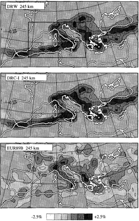
Comparing the Oercourt et al. [1986] models: ORC-I and DRC-II (7 I) A different evolution: The Dewey et al. [1989J based model DRW (72)
8 - Contents
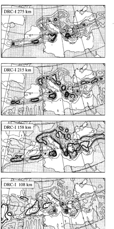
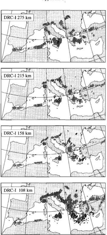
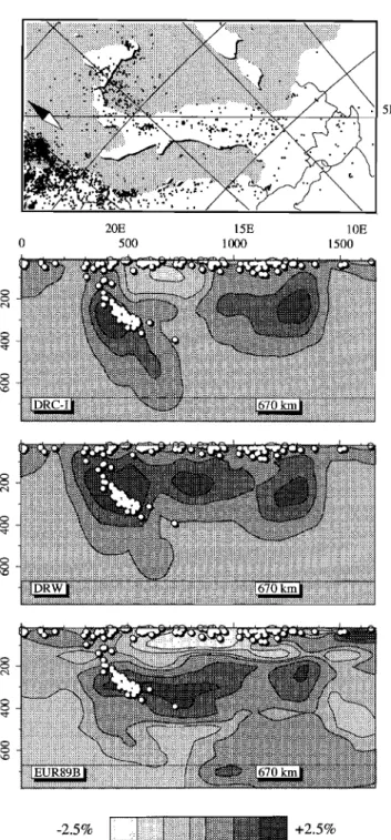
3.4 Comparing the synthetic velocity structure and tomographic results _ _ 80
Vertical Sections 80
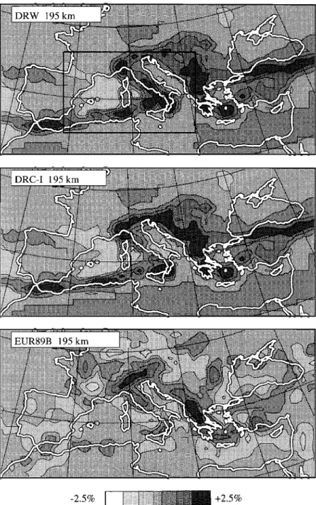
Horizontal sections 80
95 km. (81) 195km.(81) Deeper structure. (8 I)
3.5 Reliability and limitations of the modelling approach 89
3.6 Shallow detail 90
Basin subsidence 90
Heat flow density 90
3.7 Discussion and Conclusions 92
Chapter 4, Testing forward models with tomographic inversion results;
testing tomographic inversion results with forward models 97
4.1 Introduction 98
4.2 Forward and inverse models of the Alpine-Mediterranean region 100
Forward models 100
Inverse models 101
4.3 Procedure for comparison of forward and inverse models 103 Limitations of the method of resolution analysis 106 4.4 Assessing the quality of tomographic mapping 106 General experiment description 107
Experiments 113
TEST-I (113) TEST-2. (I 13) TEST-3 (I 13)
TESTA and TEST-4b (I 17) TEST-5 and TEST-5b (122) TEST-6 and TEST-6b (122) TEST-7 and TEST-7b (125) TEST-8 (125)
Conclusions on the imaging quality of the tomographic mapping 126 4.5 Assessing the quality of the tectonic reconstructions 126 Overall fit of forward and inverse results 127 Comparison of different forward models 131
Comparison of ORC-I and ORC-II (132) Comparison of ORC-I and ORW (134) Comparison of ORC-I and ORCIII (136)
4.6 Discussion and Conclusions 137
Quality of models 138
Quality of tectonic reconstructions 139
Appendix 2, Verification of
aV;aT
143Introduction
We have now another object in our view; this is to investigate the operations of the globe, at the time that the foundation of this land was laying in the waters of the ocean, and to trace the existence and the nature of things, before the present land appeared above the surface of the waters.
James Hutton, Theory of the Earth, 1788
W
ith the advent of plate tectonic theory a framework has become available in which many observed features of the structure of the Earth can be understood. The theory can explain the geological processes that have resulted in terranes as diverse as oceans, mid-oceanic ridges, mountain belts, and intra continental basins. However, despite its explanatory power plate tectonic theory is rarely used for its predictive properties, which should after all be an important aim of any scientific theory. In this research I will address someimplications of the plate tectonic concepts, by using plate tectonic theory, to predict thermal and elastic properties of the interior of the Earth which were not used to formulate the theory. This prediction is made by forward numerical modelling of lithosphere scale tectonic processes. The work will focus on the Alpine-Mediterranean region, but the method described is applicable to any part of the Earth where Mesozoic or later plate collision processes can be reconstructed with sufficient detail from geological observations.
In the past much effort has been placed in trying to understand the
complicated tectonic structures found in the Alpine-Mediterranean system and the development of this region in terms of lithospheric processes. Whereas for most parts of the world the prime source of information for reconstructing lithosphere-scale processes is the pattern of magnetic reversals of the oceanic floor, this data set is of limited use within the Mediterranean region. This is a result of the fact that oceanic lithosphere in the region shows only very little consistent magnetic structure. It falls into two categories: very young, extending -formerly continental- regions, where no clear ridges and associated magnetic patterns have (yet) developed and old Cretaceous lithosphere (dated by stratigraphic means), which was formed in the long magnetically quiet interval. Reconstructions of plate tectonic processes within this realm are therefore poorly bounded by magnetic data.
Despite the virtual absence of the oceanic data inside the region, it is possible to reconstruct the large-scale motion of the Eurasian and Mrican plates (bounding the region in the north and south) from the opening history of the Atlantic ocean [Savostin et al., 1986] and from the difference between polar wander curves of Africa and Eurasia [Westphal et al., 1986]. By cOInbining the geometrical boundary conditions given by large scale motions with information of (micro-)plate rotations, stratigraphy and structural geology
10 - Introduction
some workers have succeeded in determining a geometrically consistent descriptions of plate motions and internal deformation throughout the development of the currently observed geological structure [Dercourt et aI., 1986 and Dewey et aI., 1989].
These reconstructions are known as paleogeographic reconstructions, when the attention is mainly focused on the distribution of continental and oceanic environments, or palinspastic reconstructions when basin sedimentology and geology is the prime subject. In either case an important feature included in the recent reconstructions is the general tectonic setting of the studied region during its evolution. For the sake of uniformity I will refer to all sufficiently detailed reconstructions of geological processes as tectonic reconstructions. These reconstructions are characterised by a substantial amount of geological interpretation as many instances of oceanic lithosphere formation, subduction, and intra-plate deformation are only recognizable in the form of narrow zones of anomalous lithology in old orogenic belts. It is for example virtually impossible to accurately quantify the size of the old basins that have become incorporated in the Alps and Carpathians. Furthermore, the motion of plates or plate-fragments is often only known with a large margin of error. An important aim of this study is to assess the quality of the tectonic reconstructions by studying their implications for the underlying mantle structure. In Chapter 1 I will present a brief outline of the currently available hypotheses concerning the development of the Mediterranean region and illustrate some of the problems encountered.
In chapter 2 the forward modelling approach designed to study the implications of the tectonic reconstructions is presented. In the forward models the information implicit in the tectonic reconstructions is used to determine an unperturbed (but not necessarily homogeneous) initial mantle structure and an accompanying material flow field. It is then possible to calculate the thermal effects of the tectonic development on the underlying mantle.
The first objective of this research is testing the quality of various interpretative reconstructions by modelling their implications for the present lithosphere and upper mantle structure. The modelling approach produces predictions (from the unperturbed past situation towards the present structure) that follow from the plate tectonic assumptions and the time dependent tectonic reconstructions. It is clear that a prediction of the mantle has only limited use if it cannot be checked against observations. There is however, a means to test the predicted structure because we can compare it with the detailed seismic velocity structure of the lithosphere and upper mantle that is obtained by delay-time tomography.
The second objective of this research stems from the lack of explanatory power that seismological studies of the structure of the mantle provide. When the first experiments with seismic delay-time tomography were performed it was already suggested that the imaged lateral P-wave velocity heterogeneities were indicative for the tectonic processes in the area. [Aki et aI., 1977 and Dziewonski et aI., 1977]. In these initial studies, however, no connection
II - Introduction
between the tomographic results and the actual tectonic history could be given, either because of the small area covered or because of the low spatial resolution of the mantle images. Although the resolution and accuracy of global models improved in subsequent years [Clayton and Comer, 1984 and Dziewonski 1984], the correlation between imaged mantle P-wave velocity heterogeneities and the expected structure from plate tectonic theory remained poor.
This situation changed when results obtained by Spakman [1986] and Spakman et al. [1988] showed a clear P-velocity anomaly with a spatial extent that suggested it was directly related to a northward subduction of Mrican lithosphere below Crete. One important observation in this study was that the maximum depth of subduction is substantially larger than that of seismic events in the region. This result indicates that P-wave velocity anomalies of the mantle can reflect a much longer portion of the subduction history than earth quake hypocentre locations. The image of the Mediterranean upper mantle in this work furthermore shows a number of zones of high P-velocity that roughly follow the orogenic belts found in the region, but that were not always associated with deep seismicity. The interpretation was made that these zones were also the result of past subduction processes. This study will go a step further in the interpretation of the presently observed seismic structure. When the forward models and the tomographic results show a good correlation (a problem that will be extensively addressed in Chapter 4) we have in the underlying tectonic reconstruction a true quantitative explanation for the current seismic velocity heterogeneities. The development of the mantle towards its present structure can then be understood in terms of tectonic processes that have also left their mark in the surface geology. In this way we quantitatively verifY the tectonic processes that are responsible for the development of the complicated structure presently observed by seismological means.
A third use of the modelling approach exists from an epistemological viewpoint: especially a well established theory like plate tectonics needs to provide falsifiable predictions to be of scientific value [Popper, 1963]. It is of course beyond the scope of this research to reassess the validity of plate tectonics, but by comparing forward models and recently obtained tomographic results previously unaddressed implications of the theory can be confronted with observations. This somewhat philosophical consideration does playa role in the error discussion of chapters 3 and 4 where limitations of the modelled plate-like nature of subducted lithosphere may be part of the source of discrepancies between forward models and tomographic results. It is in those errors of the forward models that we encounter the limits of the simple plate tectonic approximation of the dynamics of the Earth and we find new questions on the nature and properties of the Earth's mantle.
12 - Introduction
References:
Aki, K., E. Husebye, and A Christofferson, Determination of the three-dimensional seismic structure ofthe lithosphere, J. Geophys. Res., 82, 277-296, 1977.
Clayton, R. W., and P. Comer, A tomographic analysis of mantle heterogeneities, Terra
Cognita, 4, 282~283, 1984.
Dercourt, J., L. P. Zonenshain, L.-E. Ricou, V. G. Kazmin, X. Le Pichon, A L. Knipper, C. Grandjacquet, I. M. Sbortshikov, J. Geyssant, C. Lepvrier, D. H. Perchersky, J. Boulin, J.-C. Sibuet, L. A Savostin, O. Sorokhtin, M. Westphal, M. L. Bazhenov, J. P. Lauer, and B. Biju-Duval, Geological evolution of the Tethys from the Atlantic to the Pamirs since the Lias, in Evolution of the Tethys, edited by J. Auboin, X. Le
Pichon, and A S. Monin, Tectonophysics, 123, 241-315, 1986.
Dewey, J. F., M. L. Helman, E. Turco, D. H. W. Hutton, and S. D. Knott, Kinematics of the western Mediterranean, in Alpine Tectonics, edited by M. P. Coward, D.
Dietrich, and R. G. Park, Spec. Publ. Geol. Soc. London, 45,265-283, 1989.
Dziewonski, A M., Mapping the lower mantle: determination of lateral heterogeneity in P velocity up to degree and order 6, J. Geophys. Res., 89, 5929-5952, 1984.
Dziewonski, AM., B. H. Hager, and R. O'Connell, Large-scale heterogeneities in the lower mantle, J. Geophys. Res., 82, 239-255, 1977.
Popper, K. L., Conjectures and refutations, the growth of scientific knowledge, Routledge and Kegan Paul Ltd., London, 1963.
Spakman, W., Subduction beneath Eurasia in connection with the Mesozoic Tethys,
Geol. Mijnbouw, 65, 145-153, 1986.
Spakman, W., M. J. R. Wortel, and N. J. Vlaar, The Hellenic subduction zone: a tomographic image and its geodynamic interpretation, Geophys. Res. Lett., 15, 60
63,1988.
Savostin, L. A, J.-C. Sibuet, L. P. Zonenshain, X. Le Pichon, M.-J. Roulet, Kinematic evolution of the Tethys belt from the Atlantic ocean to the Pamirs since the Triassic, in Evolution of the Tethys, ed. by J. Auboin, X. Le Pichon, and AS. Monin, Tectonophysics, 123, 1-35, 1986
Westphal, M., M. L. Bazhenov, J. P. Lauer, D. M. Pechersky, and J.-C. Sibuet, Paleomagnetic implications on the evolution of the Tethys belt from the Atlantic ocean to the Pamirs since the Triassic, in Evolution of the Tethys, ed. by J. Auboin,
13
14 - Chapter 1
Chapter 1
Mesozoic and Cenozoic tectonic
evolution of the
Alpine-Mediterranean region
Some think that even the ancients who lived long before the present generation, and first framed accounts of the gods, had a similar view of nature; for they made Ocean and Tethys the parents of creation, ...
Aristotle, Metaphysics, 350 E.G.
1.1 Introduction
T
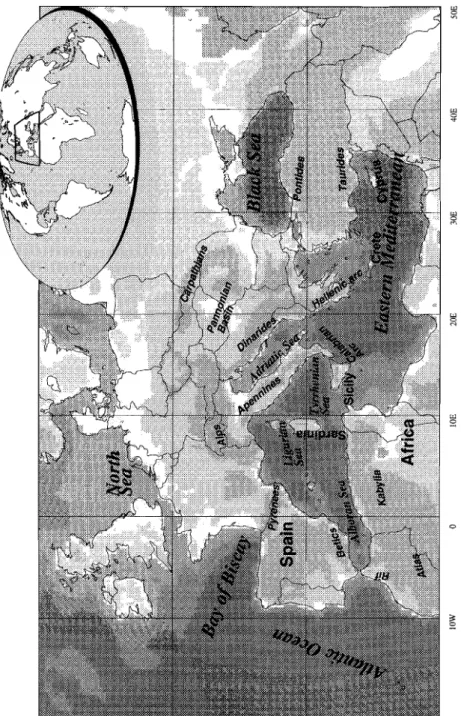
he forward modelling of tectonic processes described in the next chapters is based on tectonic reconstructions of the Alpine-Mediterranean region. Both the model kinematics and the initial mantle and lithosphere structure are derived from these reconstructions. In this chapter I will therefore present a brief synthesis of the different reconstructions. I will discuss aspects of a number of models, based on work by Dercourt et al. [1986, 1990] and Dewey et al. [1989]. These reconstructions of the tectonic evolution are currently the most widely accepted, and provide sufficient information for the forward modelling. The modelling approach could be used to test other reconstructions but it is not the aim of this study to analyse every proposed history of the Mediterranean region. Instead, I will focus on the most recent hypotheses.For orientation Figure 1 shows a map of the area addressed in this study. The tectonic processes in this region have resulted in a number of mountain belts and basins. Along the northern side the present terrane is dominated by the chains of the Pyrenees, the Alps, the Carpathians and the Pontides. These four chains delimit the northern side of the Mesozoic Tethys area. A common characteristic is the northward tectonic transport of Late-Mesozoic to Cenozoic sediments and Palaeozoic metamorphics over a presently continental basement belonging to the Eurasian mainland. A large strike-slip component of later motion on the delimiting faults is also often observed.
The southern edge of the region is dominated by the Mesozoic Atlas mountain belt of northern Africa, and by the island arcs of Sicily-Calabria, the Hellenides and Cyprus. A common characteristic of these regions is overthrusting over of various crustal fragments over the north-Mrican and southern Tethys lithosphere. In a very condensed form the history of the Mediterranean could be summarized as the subsequent creation and destruction of the Tethys ocean that was located between these two zones of
16 - Chapter 1
orogenic belts. In the interior of the Alpine-Mediterranean region other mountain chains are also present: around the Adriatic Sea the Apennines and Dinarides and around the Alboran Sea the Betic, Rif, and Kabylia mountains. Furthermore, inside the region a number of basins are found: the oceanic remnant of the Mesozoic southern Tethys in the eastern Mediterranean, the newly formed oceanic basins of the Alboran, Ligurian and Tyrrhenian Sea, the Intra-continental Pannonian basin behind the Carpathians, and the strongly extended Sea of Crete behind the Hellenic arc.
1.2 Tectonic reconstructions
ISO m.y. HKlm.y. 50 m.y.
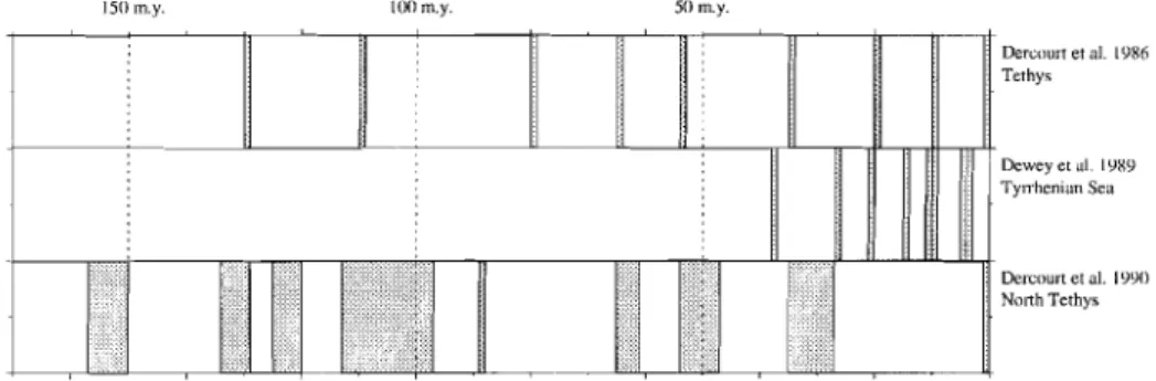
Dercourt et £II. 1986 Tethy" Dewey et £II. [~89 Tyn"henian Sea Dercourt et £II. 1990 NOith Tethys
Figure 2. Time coverage of the tectonic reconstructions considered in this study. Grey bars show the periods where maps are available.
It is no simple undertaking to assemble all these different terranes into a single scenario for their development, yet it is precisely this that the tectonic reconstructions aim to do. In this section I will briefly describe the reconstructions used in this study. These reconstructions are made by Dercourt et al. [1986], Dewey et al. [1989], and Dercourt et al. [1990]. The tectonic information is represented as a number of maps for different times in the past (see Figure 2), featuring the main tectonic structures and geography. The large scale framework of these reconstructions is essentially the same, therefore the following section will focus on one, while differences between various hypotheses will be noted when applicable.
The history of the Alpine-Mediterranean region will be considered from the early Jurassic onwards, because before this time the mantle structure is determined by a stable configuration of continental lithosphere. The breaking up of the Pangean landmass is the initial setting for the modelling of the history of the region. By Early Jurassic time the African and European shelf regions are moving with a strike slip displacement. Eastward of the modelled
17
- Tectonic evolution
in between [Savostin et aI., 1986 Westphal et aI., 1986], but this occurs outside the region of interest for this study.
Figure 3 (page 20) shows the paleogeography and main structural features and type of lithosphere taken from the Dercourt et al. [1986] reconstruction close to the Jurassic-Cretaceous boundary (130 m.y., in this study I will use absolute ages from Harland e't ai. [1982], but small differences in absolute timing of the processes will not be noticeable in the forward modelling results). The map inset is the alternative reconstruction for the Alpine region given by Dercourt et ai. [1990]. The mentioned parameters are the ones I will use in the subsequent modelling. Figure 3 shows the onset of oceanic lithosphere formation in the Western (Neo-) Tethys and Valais Trough. It is this lithosphere that will become incorporated in subduction processes later in the development. The Adriatic promontory of the African plate and the adjoining Ionian, Gavrovo and Pindos regions are still and integral part of the African shelf region, although the Lago Negro basin is already starting to form. The first subduction in the region also begins during this time that will later develop into the Dinaride and Hellenide belts (see also Figure 1 for geographic names). The formation of oceanic lithosphere continues from this time onward to the end of the Cretaceous (65 m.y.) along different ridge systems. The tectonic development at this time however, is largely determined by extension and spreading processes. Note that the amount of oceanic lithosphere present in the Valais Trough is much larger in the map inset of Figure 3 (Dercourt et al. [1990] reconstruction). The total size of the oceanic basins in the Alpine Mediterranean region is hard to assess, because subduction and oceanic lithosphere formation occur simultaneously. In this study I will use a minimum estimate for the oceanic basin surface area, but a larger amount of subducted lithosphere cannot be ruled out from the tectonic information. As a result the possibility should be taken into account that the forward models of the Alpine region show less high-velocity material than is actually present in the mantle. Between 130 and 110 m.y. the reconstructions indicate a spreading ridge active between the Ionian Trough and North-Africa, thus separating the Hellenide-Adriatic region and the latter and producing the oceanic lithosphere that is presently found in the Eastern Mediterranean basin. Around 80 m.y. the Bay of Biscay is formed by south-eastward migration and rotation of the Iberian microplate. Already during this spreading phase of the Neo-Tethys, subduction processes are thought to start consuming lithosphere along the Valais trough, Carpathian Flysch basin and Pindos suture in the northern part of the region. During the Cretaceous ocean floor formation in the South and subduction in the North continue.
Figure 4 (page 21) shows a reconstruction of a more advanced stage of the development ( 65 m.y.). This time subduction and thrusting processes occur in the region of the Kabylia mountains, where oceanic lithosphere that was formed in the Cretaceous disappears below the Iberian microplate. Northward subduction is also interpreted in the Calabrian arc (still located far west of its present position), Along the entire northern Tethys margin (Alps, Carpathians
18 - Chapter 1
and Pontides) the Austro-Alpine and adjacent regions overrides the Eurasian foreland. From this time onward to the Oligocene also the thinned continental lithosphere of the Pindos and Gavrovo zones are thought to become involved in thrusting, and to disappear below Dinarides and Hellenides. In the forward
modelling we have assumed that these thrusting processes represent subduction. Oceanic crust formation in the region has stalled. In a general
sense the plate geometry has become simpler as a result of this: the kinematics are now dominated by a two-plate Africa-Eurasia convergence.
The next maps (Figure 5, page 22) show the paleogeography at 35 m.y.. For this period we have three possible reconstructions (the lower left inset shows the Dewey et al. [1989] interpretation). This time some thrusting is given around the Iberian plate: in the Pyrenees and Betic cordillera. Soon after, the Iberian microplate becomes an integral part of the European continent. The Valais Trough has been consumed below the Alpine front. In the western
Mediterranean subduction of old oceanic lithosphere marks the beginning of the formation of the Apennines. Note that Dewey et al. [1989] suggest a different shape and position for this convergent boundary.
Tectonic activity in the Alps is present from the Oligocene until after the Tortonian (10 m.y.) as is illustrated in Figure 6 (page 23). In this period large
nappes are overthrusting the French, Swiss and Austrian molasse basins. But the type of lithosphere present at the contact has changed to continental somewhere around the early Oligocene, when the oceanic basins have been completely consumed.
The Carpathians show a similar evolution to the Alps, only the amount of oceanic crust, formed in the Cretaceous, is larger and subsequently more material gets subducted in the later stages. A difference is the typical back-arc extension that occurs during the Oligocene and Miocene in the Pannonian basin, which is not found in the Western part of the Alps. After the Oligocene subduction in the Dinarides has ceased, but further south, convergence rate along the Hellenides has increased. Also thrusting in the Pontide region is thought to have ceased while to the South the Cyprus arc and Tauride zones are still active. During the Early Miocene new oceanic crust is formed in the Ligurian Sea, because of very strong extension between Sardinia and Spain, and in the Alboran Sea. These processes started with continental rifting during the Aquitanian ( 20 m.y.). The eastward migration of the Apennine thrust front is well underway (but note the different amounts of extension at this time implicit in the Dercourt et al. [1986] and the Dewey et al. [1989] reconstructions).
The final stage of the tectonic development is shown in Figure 7 (page 24). The Tyrrhenian Sea has been formed by late stage extension (in the Late Miocene to Pliocene depending on the reconstruction considered) of the overriding plate. Thrusting in Alpine-Carpathian chains has (almost) stopped. The fastest moving plate boundary is found in the Hellenic arc system, where extension of the Sea of Crete accommodates much of the relative displacement. At present this region appears to be the only active subduction zone in the
19
- Tectonic evolution
Alpine-Mediterranean, although the possibility exists that the Calabrian arc is also still active.
In the following chapters I will test what the effects of the above described processes on the present lithosphere and mantle the above described must be, and whether these processes can explain the current seismological observations. In order to do so, the next chapter will give a description of the modelling method used to translate the tectonic hypotheses into physical processes.
po >:rj
5.
r!i1' tJ~ CD CD ;:; W o ' ~ "'d <",-po CD til ct-O poll'l_CD . 0 ~~~po ~'O 2::>" . '< § Po S po S'~
~
'"
~ > w o S ~ po ;:+> CDf
...~
CD ct ~ ~ ~ 00 ~ o ~ 'ON Oceanic ridgeIII
Convergent margins and faults Emerged landContinental shelf
!1~i~1~~J~;,i;,ili;::"ii~ii,j.iii
~~:~~n::~e::;~~~~os
phereQ
.§
~~<.Oaq 3~• <ll :I>
;p
r0 o aq <ll 0 ~~ '0 ::r '< ~ .... O"l 01 S ~ ~ ~ <ll '"1 U <ll rl 0 ~ ~ <ll .... ~ ;:;' <.0 00 23 ~ ::; 0. U <ll '"1 I> 0 ~....
<ll .... ~ 50N 25N Oceanic ridgeConvergent margins and faults Emerged land
Continental shelf Thin continental lithosphere Oceanic lithosphere ~ n 8" ;:; c:;. C\) <:: c 1::
....
c·
;:; t-.:l....
22 - Chapter 1
Figure 5. Paleogeography at 35 m.y., after Dercourt et al. [1986], Dewey et al. [1989], and Dercourt et al. [1990].
~"%j ... ~oq 00::: ~'"l ':"""'CD cr> "d o
i
~*'
o ~ ... o S ~ ~11
'"l t:l CD8
::: ;:\. ~ ~ p CD 00 ~[
t:l ~ ~ CD ... ~ 50N ;;;'l'"
~.
'"
<I> <:: ~ .::....
o·
;;l J5E Oceanic ridgeConvergent margins and faults Emerged land
Continental shelf
19
rn:y.
Deweyeta!.1289J
Thin continental lithosphereOceanic lithosphere
t>:l
24 - Chapter 1
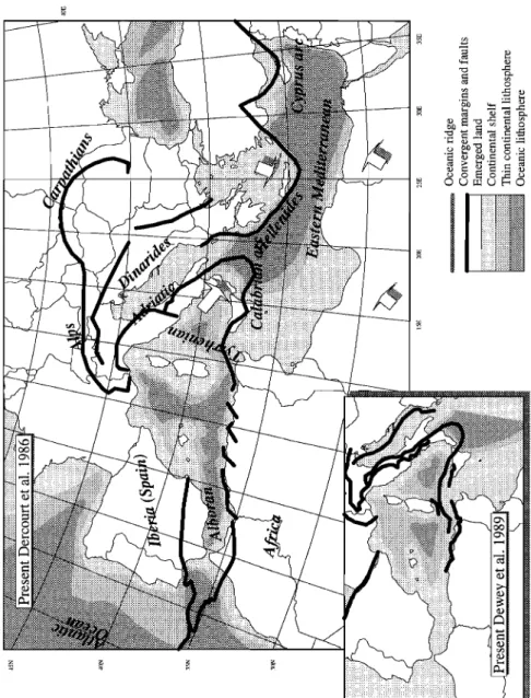
Figure 7. Present distribution of tectonic features and lithosphere types, after Dercourt et al. [1986) and Dewey et al. (1989).
25
- Tectonic evolution
References:
Dercourt, J., L. P. Zonenshain, L.-E. Ricou, V. G. Kazmin, X. Le Pichon, A L.
Knipper, C. Grandjacquet, I. M. Sbortshikov, J. Geyssant, C. Lepvrier, D. H. Perchersky, J. Boulin, J.-C. Sibuet, L. A Savostin, O. Sorokhtin, M. Westphal, M. L. Bazhenov, J. P. Lauer, and B. Biju-Duval, Geological evolution of the Tethys from the Atlantic to the Pamirs since the Lias, in Evolution of the Tethys, edited by J. AUboin, X. Le Pichon, and AS. Monin, Tectonophysics, 123,241-315, 1986. Dercourt, J., L.-E. Ricou, S. Adamia, G. Csaszar, H. Funk, J. Lefeld, M. Rakus, M.
Sandalescu, A Tollman, and P. Tchoumachenko, Anisian to Oligocene paleogeography of the European margin of Tethys (Geneva to Baku), in Evolution
of the Northern margin of the Tethys: The results of IGCP project 198, edited by M.
Rakus, J. Dercourt and A E. M. Nairn, Mem. Soc. Geol. Fr., 153(II!), 159-190, 1990. Dewey, J. F., M. L. Helman, E. Turco, D. H. W. Hutton, and S. D. Knott, Kinematics of the western Mediterranean, in Alpine Tectonics, edited by M. P. Coward, D. Dietrich, and R. G. Park, Geol. Soc. Lond. Spec. Publ., 45, 265-283, 1989.
Harland, W. B., A V. Cox, P. G. Llewellyn, C. A G. Pickton, A G. Smith, and R.
Walters, A geologic time scale, 131 pp., Cambridge Univ. press, Cambridge, 1982. Savostin, L. A, J.-C. Sibuet, L. P. Zonenshain, X. Le Pichon, M.-J. Roulet, Kinematic
evolution of the Tethys belt from the Atlantic ocean to the Pamirs since the Triassic, in Evolution of the Tethys, ed. by J. AUboin, X. Le Pichon, and AS. Monin,
Tectonophysics, 123, 1-35, 1986
Westphal, M., M. L. Bazhenov, J. P. Lauer, D. M. Pechersky, and J.-C. Sibuet, Paleomagnetic implications on the evolution of the Tethys belt from the Atlantic ocean to the Pamirs since the Triassic, in Evolution of the Tethys, ed. by J. Auboin, X. Le Pichon, and AS. Monin, Tectonophysics, 123,37-82, 1986.
Chapter
2
Thermal modelling of tectonic
processes
The forms of bodies are infinitely varied; the distribution of the heat which penetrates them seems to be arbitrary and confused; but all the inequalities are rapidly cancelled and disappear as time passes on.
Joseph Fourier, The analytical theory of heat, 1878
T
he information contained in tectonic reconstructions consists of results of a large number of geological and geophysical studies. However, in the forward modelling method described in this study, these results are treated as input data. In the modelling approach the objective is to predict physical properties of the lower lithosphere and mantle from this 'data'. In this chapter I will describe the model assumptions and calculations that are used to predict mantle and lithosphere properties from tectonic reconstructions. The method is basically the same as the one described by De Jonge and Wortel [1990].Important starting points of the modelling are the following two assumptions:
1) The structure of the lithosphere and underlying mantle are closely related. By this I mean that large scale tectonic processes, like those proposed in the tectonic reconstructions, are the surface expression of processes involving crustal, lithospheric and mantle levels of the earth. Horizontal motion of plates implies vertical displacement of material in the mantle.
II) A vertical component of motion affects the temperature distribution, because it can introduce cool lithospheric material into the mantle and it can bring hot material to the surface.
The first assumption is obvious from geometric considerations alone. When two lithospheric plates converge, the surface area destroyed is largely consumed in a subduction process. This means that surface motions of the tectonic reconstructions are associated with material flow that has a vertical component. For the same reason diverging and extending plates are accompanied by a vertical flow component. The second assumption is valid when the vertical motion takes place in a not purely adiabatic setting. Since the thermal gradient of the lithosphere is largely determined by conductive processes this condition is met when lithosphere is involved in the vertical motion (either as source or as destination of the flowing material).
A working hypothesis for this study is furthermore that the observable structure of lithosphere and mantle is strongly influenced by the temperature distribution. I consider the temperature effect as a prime cause for the observed mantle heterogeneity for a number of reasons. Firstly, subduction processes produce thermal anomalies that are associated with seismic velocity structure comparable in magnitude to seismic observations [Minear and
28 - Chapter 2
Toksoz, 1970; Sleep 1973], in other words: temperature differences suffice to explain the amplitude of the seismological structure. Secondly, the thermal effects of subduction and extension are better known and less dependent on the specific study area than compositional or anistropic features. Unlike these latter two features the temperature effect of subduction and extension is a minimum necessity (composition mayor may not affect P-wave velocity in a certain region, anisotropy mayor may not be present at a certain level, but thermal contraction or expansion is unavoidable when material moves). When I model the mantle structure as purely temperature determined the number of unknown parameters is therefore reduced to a minimum. The temperature dominance is not a required modelling assumption like the previous two, because its falsehood can be readily established by comparing model predictions and geophysical observations.
With these considerations the approach for the modelling becomes straightforward:
1 Determine an initial thermal state of the mantle (from the earliest stage of the reconstruction or from other considerations).
2 Determine the surface-displacement and deformation of lithosphere fragments through time.
3 Determine vertical flow associated with the horizontal motion.
4 Use both vertical (interpreted) and horizontal (directly from the tectonic reconstruction) material flow to displace the initial structure (stepwise through time in a numerical model).
5 Calculate diffusion of heat (after each step).
6 Calculate the effect of the present temperature structure (last step) on the required physical quantities.
In the following sections I will explain these modelling steps in more detail.
2.1 Initial thermal structure
In the tectonic reconstructions an indication is often given of the type of
lithosphere present in different parts of the region (see for example Figure 2 of the previous chapter). When oceanic lithosphere is present at the time, it is possible to determine the initial thermal structure if the reconstruction specifies the time of formation of this lithosphere. This initial structure is derived from the cooling half-space approximation with average material properties (table 1). This model yields a conductive temperature distribution which has the following form (for a derivation see for example Carslaw and Jaeger [1959] or Turcotte and Schubert [1982]):
z
T(z,t}=To erf{--) 1)
fW
In equation 1 To, denotes the mantle temperature at surface conditions
(extrapolated along an adiabat), known as potential temperature [McKenzie, 1969; 1970], z is the depth coordinate, t is the time elapsed since the formation
29
- Thermal modelling of tectonic processes
of the lithosphere, and K is the thermal diffusion parameter: k / PCp' The cooling
half-space approximation yields good predictions for basin depth and heat-flow of young oceanic lithosphere (less than 80 m.y. old), as shown by Sclater and Francheteau [1970], Sclater et al. [1971], and Trehu [1975]. For older lithosphere it is expected to be less accurate because upward heat flow from below the conductive layer is for example ignored in this expression.
Note that old oceanic basins are not present in the studied region during the Early Jurassic (following the reconstructions rifting in the region started in the Triassic), and therefore these do not constitute an 'initial' condition. In the
subsequent time-dependent thermal modelling a small net heat-low into the base of the model is included to allow for a heat contribution from the cooling core and slightly radiogenic lower mantle (both a few times 1012
W following Stacey [1992]), resulting in an upward heat flux of 10mW/m2
at the base (1000 km depth) of the forward models. As a result the modelling for old oceanic lithosphere, starting from a young initial state provides a better prediction of heat-flow density and ocean floor topography than the half-space model at a large age (but not perfect, latent heat release from solidification is for example ignored).
Table l:Physical properties for thermal modelling. Values from Turcotte and Schubert [1982], Toksoz et al. [1973]. Unit Oceanic crust and mantle (m) Lower continental crust (2) Upper continental crust (1) specific heat (cp) Jlkg,K 1050 1050 1200 conductivity expansion (k) (a) W/m,K 11K 3.34 3.610-5 3.3 1.610'5 3.0 2.4 10-5 density (p) kg/m3 3400 2900 2650 heat prod. (H) Wlkg 0 10-11 10-9
Initial temperature structure in continental regions is calculated with a steady state approximation of a typical three layer continental model. Figure 1 shows the expressions used to determine the initial geotherm. The thermal parameters and symbols are shown in Table 1. The values for this modelling are average for a crust with an upper part of granitic and a lower part of an average diorite and amphibolite composition, comparable with values given by Rybach [1987]. The parameter that is required from the tectonic reconstructions is an estimate of the total thickness of the continental crust, which we obtain by combining the paleo-position of continental areas and indications of lithosphere type from the reconstructions with present crustal thickness information from Meissner et al. [1987] shown in Figure 2. Note that this present crustal thickness can only be used for terranes that have not been
30 - Chapter 2
changed by tectonic processes during the period we intend to model. In other cases the thickness is estimated from adjacent regions.
Z=O, T=To
T I , AI, k] T](z)~o -(A]/2k]) Z2 +(qm+A2d+A]d)/k] Z
Z=2d
T2, Al, k2 Tiz)~](d)-(Ai2k2) (Z_d)2 +(qm+A2d)/k2 (z-d)
Figure 1. Schematic view and equation 2) for a I-dimensional steady-state continental model with two layers of constant radiogenic heat production.
The mantle contribution of heat flow for the initial continental models is kept at a fixed value of 21 mW/m2, corresponding to the adiabatic gradient in the
underlying asthenosphere [Anderson, 1981]. This is only the initial and steady state value, the heat flow, and subsequently the continental geotherm, are free to change in the modelling (although of course they will not do so if no material flow is occurring).
For both continental and oceanic regions the underlying mantle temperatures are calculated using an adiabatic temperature rise with depth (Equation 3). This expression yields the temperature at a given depth, from the potential temperature Tp [McKenzie, 1970]. p T is also the temperature determined with Equations 1 and 2 in the conductive part of the model, it is 1600K below the conductive part if no perturbations are present (e.g. Anderson [1981], Turcotte and Schubert [1982]).
31
- Thermal modelling of tectonic processes
SON
40N
30N
o
toE 20E 30EFigure 2. Thickness of crust (including sedimentary cover) after Meissner et al.
(1978).
za.g
p 3)
T(z)=T/z)e C
In Equation 3, g is the gravitational acceleration, a the thermal expansion coefficient, Cp the specific heat, and T is expressed as absolute temperature.
The mantle temperatures are furthermore corrected with phase transition effects. A second order polynomial approximation for the depth of the 400km phase transition and a linear estimate for the depth of the 670km transition are used. These two corrections simulate phase transition effects by increasing the temperature with 150 K below both transitions at a depth that depends (mildly) on temperature. The parameters for these effects are shown in table 2. The depth and latent heat release of the 400 km discontinuity are fairly well established (see for example Anderson [1989] or Turcotte and Schubert [1982]). The value for the 670 km discontinuity is less well constrained. Estimates for the slope of the Clapeyron line for the transition from y-spinel to silicate perovskite plus magnesiowllstite are uncertain. In. this study I will approximate this process with a simple linear estimate for the depth of this transition, based on seismological data. The depth of transition shown in table 2 is chosen so that a 1000K colder slab produces a depression in the phase boundary of 30 km [Barley et al., 1982; Richards and Wicks, 1990]. This may be a low estimate, as more recent work [Wicks and Richards, 1993] indicates a larger (46 to 80km) downward deflection for the comparably cold Izu-Bonin subduction zone. The entropy change for this transition is estimated to be
32 - Chapter 2
somewhat less than that of the 400 km transition [Navrotsky and Akaogi, 1984] but the ambient temperature at which the entropy change occurs is higher. Therefore I will assume that the latent heat released (TAS) also increases the temperature by 150K (TAS/cp )' Turcotte and Schubert [1982] arrive at a larger effect of 200K based on a different estimate for TAS, but uncertainties in the thermodynamic properties are so large that this is can be regarded as essentially equivalent.
The modelling of phase transitions as abrupt temperature increases and the superposition of an adiabatic temperature rise on the geotherm implies that material is convecting freely in the model. The instantaneous temperature rise approximation in fact implies an isentropic flow [Turcotte and Schubert,1971]. This is valid for subduction zones, where material moves with a relatively high vertical velocity component. For the other parts of the mantle it is likely, given typical convection velocities, that the temperature rise occurs in a zone with a width of up to 50 km [Turcotte and Schubert, 1971]. Note that the uncertainties in these phase transitions is significant for the modelled temperature distribution, but for the seismic velocity anomalies, the quantity that will actually compared to observations, their contribution is much less important. The reason for this will become apparent in section 2.4, where the expression for the seismic velocity perturbation is discussed.
With the material properties and approximations mentioned, the thermal structure at the beginning of the tectonic reconstruction is determined. Figure 3 shows a combination of the possible initial structures found in the modelling. Here, the vertical temperature distribution is calculated with the above mentioned equations for oceanic and continental lithosphere. From these geotherms it is clear that especially the age of oceanic lithosphere will have an important impact on the thermal structure. The fact that continental lithosphere is present in a region is also important, but the actual thickness of the continental crust will have a much smaller effect on the thermal structure.
Table 2. Temperature effect and depth of phase transitions as a function of temperature.
Transition LlT depth of transition Olivine-spinel +150 K
'400 km'
Spinel-perovskite + +150 K 700-T*1.5 10-2 km
-33
- Thermal modelling of tectonic processes
Oceanic geotherms ,Continental geotherms
o o N Age of lithosphere --- 3m.y. o - - - 30 m.y. o 00 90m.y. 60km 36 km 2lkm I Crustal thickness 500 1000 1500 500 1000 1500
Temperature (0C) Temperature (OC)
Figure 3. Initial geotherms for oceanic and continental lithosphere.
2.2 Determining a kinematic model from a
tectonic reconstruction
The second step of the modelling requires information on the time-dependent displacement of material that is (implicitly) given in the tectonic reconstruction. I will discern two important categories of kinematic processes that influence the mantle and lithosphere structure: relative convergence between plates and intra-plate extension.
34 - Chapter 2
Convergent plate boundaries.
The relative motion occurring when two plates converge is considered to be accommodated at a subduction zone located at the (time-dependent) position taken from the tectonic reconstruction. As I will model the thermal effects of subduction in two-dimensional sections, the relevant parameters for this modelling are the component of the convergence rate parallel to the plane of the vertical section, and the angle under which the lithosphere is subducting in this section.
LowerPl\
Trench all-At
Point at t-~t
Point at t~~1
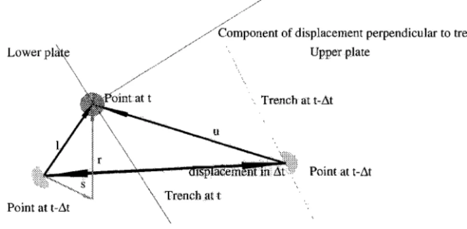
Figure 4. Determination of the convergence rate of a subduction zone from the tectonic reconstruction in the time interval t-~tto t.
The convergence rate of subduction zones is determined from the reconstruction in the following manner: Rigid body motion of the subducting plate for a given point of the plate are given by the rotation of the lower plate as reconstructed from Paleomagnetic data. For the Dercourt et al. [1986] reconstruction, Savostin et al. [1986] specify Paleomagnetic rotation poles relative to Eurasia for the African, Adriatic, and Iberian plates. Similar data are available in the Dewey et al. [1989] reconstruction. The incremental -i.e. for a small time step- rotation of a point at the trench gives the lower plate motion vector relative to this point (1'). When the subducting plate shows an active oceanic ridge a vector (8) representing the ocean floor spreading during the time step is added to this motion vector. These two contributions comprise the rigid body motion of the lower plate (t) at the subduction zone (see Figure 4 for the symbols).
During the time step evaluated the upper plate may also have moved (either rigidly or as a result of intra-plate deformation). This motion
eli
in Figure 4) can be derived directly from the position of the trench indicated in thepaleogeographic maps. The convergence velocity at the trench is now given by
35 - Thermal modelling of tectonic processes
magnitude of the time step. The component of this motion perpendicular to the trench is the controlling rate of convergence used in the thermal modelling of the subduction zone, because it is this component that determines how much lithosphere must have been subducted in the time interval. Note that the vectors shown if Figure 4 are calculated for motions on a spherical earth, not as vectors in a flat plane. Furthermore, the time intervals used for the evaluation need not be equal to those of the tectonic reconstruction (like those shown in Chapter 1, Figure 2): in cases where the reconstruction shows large gaps the trench position has been interpolated (linearly between the known times). This is not quite the same as interpolating the resultant relative velocities derived from a large displacement and time step, as both the changing trench geometry and the plate rotation have complicated effects on the magnitude of the relative motion.
The convergence rate determined in this manner for different reconstructions of the studied area can vary strongly, both in space and in time. Figure 5 shows a few representative cases derived from the Dercourt et al. [1986] and the Dewey et al. [1989] reconstructions. In these figures the height of the bars denotes the perpendicular rate of convergence, while the horizontal position of the bar on the map gives the position of the subduction zone at the pertaining time. These figures show the convergence at the Tyrrhenian plate boundary, which is dominated by the outward migration of the Apennine-Calabrian system.
The second parameter controlling subduction processes is the angle under which the subducted lithosphere disappears into the mantle. In this study this angle is determined from the average type of lithosphere that has subducted. For the old oceanic basins (formed in or before the early Cretaceous, and only recently subducting) the angle was estimated to be 700
Younger oceanic basins
•
are modelled with smaller dip angles, down to 300
for subduction zones with an average age of the descending lithosphere of 20 m.y.. In those cases where the reconstruction implies the disappearance of substantial amounts of continental lithosphere an angle down to 300
is also used.
The determination of the dip angle from lithosphere properties has the disadvantage that the true dip of a subduction zone may not always be modelled correctly. However, the alternative -using the present dip angle from seismological data- would imply that seismological information is used in the forward models. I have deliberately avoided this circular reference because forward models will be compared to seismological results. Furthermore the present dip angle of Benioff zones is ill-constrained for many parts of the region. The primary quantities that will be addressed in this study are strongly controlled by the bulk amount of subducted lithosphere and the residence time of this material in the mantle. Neither of these properties is strongly dependent on small errors in the dip angle.
36 - Chapter 2
34m.y.
IOm.y. IOm.y.
2 m.y. Data derived from Dewey et al. [1989] 2 m.y. Data derived from Dercourt et al. [1986]
Figure 5. Perpendicular component of the relative convergence rate for three times and two tectonic reconstructions. Shading levels at 1 cm/yr intervals.
Intra-plate extension
The second process that will be evaluated in the forward modelling is extension of lithosphere. This process occurs in many parts of the Alpine Mediterranean region, predominantly in the form of back-arc type regions on the overriding continental plate of subduction/convergence systems (eg. Western Mediterranean and Tyrrhenian region, Aegean Sea, and Pannonian basin). The material flow can be approximated with a pure shear type of deformation leg.McKenzie, 1978].
Note that it is not my intention to claim that pure-shear is the actual mode of deformation in all modelled extensional regions. This approximation is chosen because the scale of features I intend to study is such that only average
thermal effects on the scale of ten kilometres are needed, at that scale the
37
- Thermal modelling of tectonic processes
shear deformation. Furthermore, this approximation is computationally less intensive than simple shear models and it requires one less unconstrained assumption in the forward models (the nature of the extension fault).
The amount of extension is derived from the tectonic reconstruction by comparing the size of basins in the different stages of the development in the way shown in Figure 6. The modelling of extension is also done in a vertical section. The change in basin width in this section between two successive stages of the development determines the stretching factor (P). The vertical flow of material is determined by filling in the space created by lithospheric thinning with material from the asthenosphere below and on the sides of the basin.
Figure 6. Modelling of (back-arc) extension process in time interval t-l:..t to t.
With the initial structure derived from the tectonic reconstruction as in section 2.1 and the kinematics derived from the reconstruction derived as indicated in this section it is now possible to calculate the thermal effects of the lithosphere scale tectonic processes by numerical means.
2.3 Calculating the thermal development from the
initial structure and the kinematic model
The thermal structure of a two-dimensional section of the study area is calculated in a way similar to the subduction zone modelling method published by Minear and Toks6z [1970] and Toksoz et al. [1971, 19731. In this modelling the vertical section is subdivided in a large (400x200 in this study) number of cells. The initial temperature distribution is mapped to this grid. The motion of the subduction process is then modelled by shifting this temperature along a path determined by the dip angle of the slab, with a rate determined by the convergence rate of the subduction zone. Extension processes are modelled by shifting temperature (and material parameters of the crustal rocks) in
38 - Chapter 2
accordance with the (incremental) stretching factor (See Figure 7).
-v
-
--
'I'
- IEx ensiOI flow
V V
Subc uctiOI flow
V V V
T.
T
l ' ... I,J ... ... 1+ ,JV V
V
'lIII' 'lIII'...
....
-T
i,j+1V
Figure 7. Material displacement derived from the tectonic reconstruction for a vertical section in the thermal modelling.
The thermal diffusion is calculated after each time step using a finite difference solution of the thermal problem (Equation 4).
aT
=
~\;pi + ~ 4)at
pCp cpIn the current models A is only non zero for the crustal parts of continental models (radiogenic heat production is ignored for mantle material). Limited subduction of continental crust may have occurred in the Adriatic and Alpine region. In the modelling the contribution to the thermal structure is only evaluated for the upper 100km of the model, below this depth the properties of the mantle are considered identical for all cells. Boundary conditions for the thermal calculation consist of a fixed temperature of
oDe
at the top, no heat flow through the left and right hand sides, and a constant heat flux at the bottom (to simulate the effect of a cooling core and lower mantle radiogenic heat production)For computation this equation is discretized in a manner originally proposed by Douglas [1955], Peaceman and Rachford [1955], this method is known as the A(lternating) D(irection) I(mplicit) method, which has stability and convergence
properties comparable to a two-dimensional Crank-Nicholson operator, but at
- Thermal modelling of tectonic processes - 39
the equations resulting from this discretization in the case of zero heat production and constant material properties. Equation 4 then reduces, after some rearranging to:
V2T=! aT (with
K=~)
K
at
pCpWith the A.D.I. discretization the V2 and alot operators are approximated with a two-step finite difference form, the two steps being:
T *n+ I_Tn T. 1·-2T .. +T. l ' T .. I-2T.,+T., I*n+I *n+l *n+l n n n
I i,j i,j 1- J IJ 1+ J + IJ - IJ IJ + K t::.t (~)2 (t::.y)2 and yn.+.I_T~. T: n+~-2T*~:1+T:n+~ T~.+1 _2yn.+.l +T~.+I I IJ IJ 1-1J IJ 1+IJ + IJ -1 IJ IJ +1 K t::.t (Llx)2 (t::.y)2
Rearranging and grouping K, Lit, LIx, and Lly in the parameters A. and J1 (l+2KLltl Llx2
and 1+2KLlt I LlY respectively) yields:
*n+I *n+I *n+I n n n
T. I·-AT .. +T. 1 .=T.. 1+/lT ..+T.. 1
1- J IJ 1+ J IJ- IJ IJ+
and
In these Equations the
iJ
indices denote the grid points of the modelling, the n-index is for the total time step (=2Llt), and T'is an intermediate temperature solution (with no direct physical significance). Performing these two steps in succession is the identical to calculating one two-dimensional diffusion step. However, the advantage (over a standard 2D Crank-Nicholson operator) of the expressions above is that for the two half-steps the solution of both T*II+1 andT'+1 (from T' and T"1I+1 respectively) requires only the -computationally very
efficient- inversion of tri-diagonal matrices. This means that an implicit solution for the forward stepping of a large number of high resolution sections becomes computationally well feasible. A minor disadvantage of the method is the necessity to maintain more storage space (T"1I+1 needs to be kept available between steps).
The alternation of a displacement step (where the temperatures are shifted
like in Figure 7) and a diffusion calculation in the above described manner results in a numerical estimate for the development of the temperatures in the
40 - Chapter 2
vertical section throughout the tectonic history. The final stages of the development of the vertical cross-sections are combined into a three dimensional model by mapping the calculated temperatures into a three dimensional cell model. Because the thermal modelling results will be compared to results from delay-time tomography obtained by Spakman [1993] and Remkes and Spakman [1994], the cells of the three-dimensional model are chosen so that they coincide with their tomographic models. In practice this means that a number of temperatures of the two-dimensional section are averaged, since the tomographic model uses larger cells (Figure 8). As a result the detail of the forward models is reduced to what the tomographic cell volume can contain.
Note that the mapping of thermal results to the coarser grid should only be done for comparison of P-wave velocities. Other temperature dependent parameters should be derived from the higher resolution thermal results directly. In Appendix 1 at the end of this chapter I will describe the resulting temperature model. This model is projected on a much finer grid (O.2XO.2 degrees) to illustrate the attainable resolution of the synthetic models
Figure 8. Three-dimensional cell model for the seismic velocity structure. Lines on the surface denote the traces of the vertical sections calculated in modelling the Dercourt et al. (1986) reconstruction (and that are combined into the 3D model).
41 - Thermal modelling of tectonic processes
2.4 Determining thermally controlled quantities
The calculated present thermal structure cannot be compared directly with observations of the lithosphere and mantle properties. Instead derived quantities are used to compare predictions with observations. In this study three quantities will be addressed in more detail:- Basement heat-flow density: a prediction of the present shallow structure. This quantity is an almost direct translation of the temperature of the top layers of the model.
- Subsidence of extensional basins: a prediction of the time integrated shallow structure. This quantity requires some additional assumptions on material properties (density, expansion).
- P-wave velocity structure: a prediction of the -present- whole-volume structure. This quantity contains the most complete information on the mantle structure, but it also requires more 'post-processing' of the model temperatures than the previous two. In this study the focus of attention will be on the P-wave velocity structure because this quantity holds information on the whole mantle structure and its evolution, whereas the other two only give a constraint for the integrated properties of the shallow present-day structure.
Basement heat flow density
The temperature in the upper layers of the model follows from thermal calculations. In this study the surface heat-flow is free to change (the boundary condition for the top model layer is a fixed temperature of O°C). Therefore it is possible to calculate the average heat-flow density from the temperature gradient and the crustal composition (Equation 5):
q=lkT(z+Llz)-T(z)
I
5)Llz
Heat-flow density is most strongly determined by late stages of extensional deformation, as these have a strong impact on the near surface temperature gradient. In Chapter 3 I will show the results of this approximation for two different reconstructions of the development of the Tyrrhenian sea. Physically, the modelled heat-flow density corresponds to the basement contribution in a sedimentary basin with an average granitic composition. A sedimentary cover is not included in the calculation. This is not a very important omission as, for sediments, a cover with a thickness d gives an maximum additional heat flow contribution of A.d W/m2
• A quick calculation shows that the neglected additional heat flow is of the order 1.5 mW/m2
for every kilometre of average sediment in an old sedimentary basin (which is 2% of the typical total of 70mW/m2
). In fact, in the Mediterranean region it will often be much less (and
sometimes even negative) as the thermal structure has not yet reached an equilibrium (a result of high sedimentation rates [Hutchinson et aI., 1985].) Since the small-scale heterogeneity and uncertainty resulting from local fluid circulation and local geological structure in the observed heat flow is generally
42 - Chapter 2
much larger than the possible few percents error in the predicted heat flow, the sedimentary cover contribution can be ignored for regional scale modelling.
Basin topography
The second parameter than can be obtained from the temperature distribution is the subsidence of the basement as a result of stretching and subsequent temperature development. This parameter is derived from a simple local isostasy approximation. For the calculation of subsidence the following is assumed:
- Lithostatic pressure is constant (both laterally and through time) at a large depth.
- Elastic strength of interesting -i.e. strongly extending- regions is negligible (note that this is not the case if one wants to study basin edges, on- and offlap sequences or small-scale synthetic stratigraphy, but these phenomena are beyond the scope of this study).
Both these assumptions are of course only approximations of the real situation, but the main features of extensional basins should be predicted to the amount of detail present in the tectonic reconstruction.
The lithostatic pressure is found by numerically integrating the weight of a vertical column of material, down to a compensation depth of 200 kIn. If the pressure at this depth has changed from the previous time step, the amount of material added to or removed from the base of the column determines the subsidence in the way shown in Equation 6 and Figure 9:
6)
i--
(T+T 1)[with: P(t) =LJ gLlyp;O -cx} } j+ ) ]
}=o 2
In Equation 6 the m-indices denote values at the compensation depth, the j grid index runs from the surface (0) down to this value.
g is the average gravitational acceleration,
p and C( depend on the composition (like
shown in table 1 of this chapter). L1y is the thickness of the layer for which the quantities hold. L1H then equals the subsidence for a column with a basin infill with density Pr (in this study the density of water). The subsidence calculated in this way is a prediction of the back-stripped,
water loaded, subsidence of the modelled
basin (see for an example Sleep [1971] or
1-81 Figure 9. balance.
t Isostasy with pressure