Choosing the proper link function for binary data

(1)

Copyright by Jingwei Li

(2)

The Report Committee for Jingwei Li

Certifies that this is the approved version of the following report:

Choosing the Proper Link Function for Binary Data

APPROVED BY

SUPERVISING COMMITTEE:

Daniel A. Powers

Matthew Hersh

(3)

Choosing the Proper Link Function for Binary Data

by

Jingwei Li, B.M.S.; M.M.S.

Report

Presented to the Faculty of the Graduate School of The University of Texas at Austin

in Partial Fulfillment of the Requirements

for the Degree of

Master of Science in Statistics

The University of Texas at Austin

May, 2014

(4)

Acknowledgements

I would like to take this opportunity to express my deepest gratitude to Dr. Daniel Powers who has walked me through the whole journey of this master report. Without his in-depth knowledge and patient guidance it would be impossible for me to finish this study. I also would like to thank Dr. Matthew Hersh who has been my instructor since I joined the statistics program. His broad knowledge has inspired me to study and research.

I would like to thank all the faculty members who have taught my courses, including Dr. Michael Daniels, Dr. Tiffany Whittaker and Dr. Keenan Pituch who introduced me to the statistical modeling and programming and helped to build a foundation of the whole study.

A special thank-you note goes to our dearest graduate coordinator and administrative manager, Ms. Vicki Keller, who is always my go-to person for any program related questions and issues. Your prompt response, understanding of the systems, friendly yet professional dealing with issues have helped me overcome all the hurdles and continue my study successfully.

Finally I would like to thank my family and many friends who always give me encouragement and support.

(5)

Abstract

Choosing the Proper Link Function for Binary Data

Jingwei Li, M.S.Stat

The University of Texas at Austin, 2014

Supervisor: Daniel A. Powers

Since generalized linear model (GLM) with binary response variable is widely used in many disciplines, many efforts have been made to construct a fit model. However, little attention is paid to the link functions, which play a critical role in GLM model. In this article, we compared three link functions and evaluated different model selection methods based on these three link functions. Also, we provided some suggestions on how to choose the proper link function for binary data.

(6)

List of Tables

Table 2.1 Binomial link functions ... 5

Table 2.2 Link functions and the corresponding distributions ... 5

Table 4.1 Age of Menarche ... 11

Table 4.2 Adult Beetle Mortality ... 12

Table 5.1 Predicted values for Age of Menarche data ... 14

Table 5.2 Information indexes for Age of Menarche data ... 15

Table 5.3 Predict values for Adult Beetle Mortality data ... 16

Table 5.4 Information indexes for Adult Beetle Mortality models ... 16

Table 5.5 Posterior summary for p.chisq ... 19

Table 5.6 Age of Menarche ... 21

Table 5.7 Adult Beetle Mortality ... 21

(8)

List of Figures

Figure 2.1 Cumulative density functions corresponding to the logit, probit and

complementary log-log link functions. ... 6

Figure 4.1 Success rate verses continuous predict variable ... 12

Figure 5.1 ROC for Age of Menarche ... 20

Figure 5.2 ROC for Adult Beetle Mortality ... 21

(9)

1. Introduction

Generalized linear models (GLM) are often used in analyzing binary response data. One key aspect for building a satisfactory model is choosing a proper link function. A link function is the function g( ) that links the linear model specified in the design matrix (or linear predictor), where columns represent the matrix of predictor variables ( ) and rows the true parameters ( ) to the conditional mean of response variable μ. However, the choice of the link function is often made arbitrarily. Researchers tend to adopt the logit link for binary response data, since the logit link has a closed form and also generates easy to interpret results in the form of log odds and odds ratios. But logit link function cannot guarantee a good fit for all binary response data. We need to find out an efficient way to distinguish better link in statistic practice.

In this report, I applied three different methods to compare models with different link functions. First approach uses the information indexes, which includes Bayesian information criterion (BIC) and Akaike information criterion (AIC). The second method involves evaluation of the posterior predictive distribution in a Bayesian approach. Finally, I applied a receiver operating characteristic (ROC) analysis to compare three common link functions, which are the logit link, the probit link and the complementary log-log link in a binary regression. For a more comprehensive description of the difference within these common link functions, I applied analysis to two different datasets. At the end of this article, I divided these datasets into two different categories and introduced two families of transformations which may fit better for the two categories.

(10)

The main purpose of this report is twofold: 1) to use real data to demonstrate the effectiveness of different model comparing approach; 2) to provide some suggestions for choosing proper link functions.

This report is organized as follows: I will first discuss the role of link functions in GLM models and the characteristics of link functions in Section 2 and review different approaches for model comparison in Section 3. Then I will introduce two datasets for analysis and demonstrate the difference of these two datasets in Section 4 and compare three link functions will been proposed in Section 5. In Section 6, I will introduce two transformation families for binary response data, and Section 7 will be the conclusion section.

(11)

2. Link Functions for Binary Data

In this section, we will introduce the generalized linear model and three common link functions for binary response data. Also, we will talk about different characteristics of these three link functions.

2.1GENERALIZED LINEAR MODEL

Generalized linear models[1]_{are frequently used to model the dependence of a}

response variable Y on a set of possible explanatory variables , ,…, . In its simplest form, the generalized linear model is specified by:

(i) independent observations ,…, distributed according to an exponential family distribution,

(ii) a set of explanatory variables X, available for each observation, describing the systematic linear component through g[E(Y|X)] = g(μ) = , and

(iii) the link function g(μ) relating the conditional mean response μ of an observation to the systematic linear component .

To find an appropriate generalized linear model for regression data involves choosing the independent variables, the link function and the variance function. In this article, I am focus on the different choice of the link functions in binary and binomial response models.

2.2LINK FUNCTION

A link function is the function that links the linear model to the conditional mean response. The critical role that link function plays in GLM is linking the actual Y to the E(Y|X) = μ using a transformation, or linking function, that will allow the parameter range to be unbounded (from negative infinity to positive infinity) while ensuring that the model predictions will be in the plausible range. For example, in binary response models,

(12)

μ is a vector of probabilities, each element of which must be in the interval [0,1]. A proper link function will guarantee that regardless of the input, the model will produce predictions in the proper range. Also, without a properly specified link, the constant variance assumption of residuals will be violated. Because the observed Y has only two possible values 0 and 1, the residuals have only two possible values for each observation. With only two possible values, the residuals cannot be normally distributed. Moreover, the best line to describe the relationship between X and E(Y |X) is not likely to be linear, but rather an S-shape.

In GLM, there are link functions called canonical links[2]_{for different}

distributions, such as logit link for binomial regression, log link for Poisson regression and inverse squared link for inverse Gaussian distribution. However, there are still many functions other than these canonical links that also can map the systematic linear component onto the interval [0, 1]. Also, Even though GLM’s with canonical links, such as the logit link in binomial regression, guarantee maximum information and a simple interpretation of the regression parameters, they do not always provide the best fit available to a given data set. Usually, the choice of link function is arbitrary, but link misspecification can lead to substantial bias in the regression parameters and the mean response estimates[3]_{. Thus, how to choose a proper link is still important.}

In this article, I consider comparing three link functions, which are logit, probit and complementary log-log. See Table 2.1 for details. Logit link is the canonical link function for binary response data, but the probit is also popular, or there are other options that are sometimes used, such as the complementary log -log.

(13)

Link (μ) logit probit complementary log-log log[μ/(1-μ)] log[-log(1-μ)]

is cumulative standard normal distribution function Table 2.1 Binomial link functions

The distributions of the conditional mean responses (or error distribution) implied by these three link function are logistic, normal and extreme value, respectively. The mean and variances of these three distributions are different. See Table 2.2 for details.

Link Distribution Mean Variance

logit Logistic 0

probit Normal 0 1

complementary log-log Extreme-value

Table 2.2 Link functions and the corresponding distributions

Here is the Euler constant, for the complementary log-log function a possible shift in location will happen when estimating parameters.

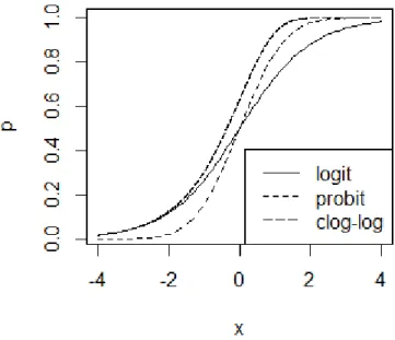
The cumulative density function plot below shows three functions are all S-shaped. Logit and probit links are both symmetrical while complementary log-log link is asymmetric. It starts pulling away from 0 earlier, but more slowly, and approaches close to 1 and then turns sharply.

(14)

Figure 2.1 Cumulative density functions corresponding to the logit, probit and complementary log-log link functions.

(15)

3. Link Comparison

Typically, different models are compared by using individual significance tests based on the asymptotic distribution of the deviance, which is called chi-square difference test (or likelihood ratio test). But this strategy cannot be used for comparing non-nested models[4]_{. Some other model comparison technics can avoid this difficulty. I}

use information indexes such as Bayesian information criterion (BIC) and Akaike information criterion (AIC) to compare models with different link functions. Also a Bayesian approach involving predictive posterior checks can compare non-nested models. Furthermore, since the response variable only value 0 or 1, so we can construct a classification table, using receiver operating characteristic (ROC) analysis applied to demonstrate how well a model predicts future outcomes.

3.1COMPARE LINK FUNCTION VIA BAYESIAN APPROACH

In Bayesian theory, predictions of future observables are based on predictive distributions which refer to the distribution of the data averaged over all possible parameter values. For this reason, when data have not been observed yet, predictions are based on the marginal likelihood

∫ | , (3.1) which is the likelihood averaged over all values supported by our prior beliefs. Hence, is also called “prior predictive distribution”.

Following the above logic, we can calculate the prediction of future data after having observed data

| ∫ | | , (3.2) which is the likelihood of the future data averaged over the posterior distribution

(16)

According to Press (1989)[5]_{inference must be based on predictive distributions}

since they involve observables while the posterior distribution also involves parameters which we are never observed. Hence, by using the predictive distribution we can quantify our knowledge about future as well as measure the probability of re-observing in the future each assuming that the adopted model true. For this reason, we may use the predictive distribution not only to predict future observations but also to construct goodness of fit diagnostics and perform model checks for each model’s structural assumptions.

The replicated data reflect the expected observations after replicating our experiment in the future, having already observed y and assuming that the adopted model is true. If the adopted model is appropriate for describing the observed data then the vectors y and will be close. Such a comparison can be facilitated by considering summary functions which play the role of a test statistic for checking the assumption under investigation and measure discrepancies between the data and the model. Assessment of the posterior distributions of _and_provides individual as well as overall goodness of fit measures which can be summarized graphically or using tail area probabilities called posterior predictive p-values given by

_|_(3.3) Here we use a type of statistic as the test statistic.

∑ | _| (3.4) The posterior p-value is obtained by

(17)

indicate that the distributions of the replicated and actual data are close while values close to zero or one indicate difference between them.

3.2MODEL EVALUATION VIA ROCANALYSIS

Receiver operating characteristic (ROC)[6] _{analysis provides a systematic tool for}

quantifying the impact of variability among individuals’ decision thresholds. Sensitivity and specificity are the most commonly used measures of detection accuracy.

(3.6)

(3.7) In effect, sensitivity and specificity represent two kinds of accuracy: the first for actually positive cases and the second for actually negative cases.

Accuracy, or the fraction of the study population that is decided correctly, is related to sensitivity and specificity by the simple formula:

(3.8)

From a binary regression model, we can make a replicate outcome variable _. The classification table below shows the how ROC analysis works in goodness of fit analysis.

(18)

1 0 total ₁ 0 total | (3.9) | (3.10) _| _| _(3.11) While only comparing accuracy is insufficient in determining a better model, models with same accuracy can have different sensitivity and specificity. We may apply different weights to sensitivity and specificity. If we change the decision threshold to several levels, we will obtain several related sets of decision fractions. We need to keep track of how sensitivity and specificity change as the decision threshold is varied. We will get the receiver operation characteristic (ROC) curve, which represents all possible combinations of sensitivity and specificity.

We can use accuracy and area under ROC curve to compare models with different link functions.

(19)

4. Data

I used two different datasets to demonstrate the difference across the link functions. These two datasets are both have binary dependent variables and only one continuous independent variable.

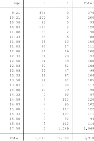
The first dataset is called “Age of Menarche,” originally reported by Milicer and Szczotka(1966)[7]_{. They analyzed data determining the age of menarche in a sample}

of 3,918 Warsaw girls. The data are reported in Table 4.1.

Table 4.1 Age of Menarche

The second dataset is “Adult Beetle Mortality.” This dataset is reported by Bliss (1935)[8]_{in a study of adult beetle mortality after five hours’ exposure to gaseous carbon}

disulphide. The data are reported in Table 4.2. Total 1,610 2,308 3,918 17.58 0 1,049 1,049 15.83 2 112 114 15.58 2 92 94 15.33 4 107 111 15.08 5 117 122 14.83 7 95 102 14.58 7 113 120 14.33 7 90 97 14.08 19 79 98 13.83 29 88 117 13.58 24 81 105 13.33 39 67 106 13.08 52 47 99 12.83 57 51 108 12.58 61 39 100 12.33 64 29 93 12.08 84 16 100 11.83 94 17 111 11.58 95 10 105 11.33 83 5 88 11.08 88 2 90 10.83 118 2 120 10.58 93 0 93 10.21 200 0 200 9.21 376 0 376 age 0 1 Total obs

(20)

Table 4.2 Adult Beetle Mortality

In the first dataset, the observed value represents the number of girls who menstruate, and in the second dataset, the observed value represents the number of adult beetles who are killed. By plotting the percentage of observed versus the explanatory variables as shown in Figure 4.1 below, I found these two curves are different. The dose response curve seems skewed while the age curve is symmetric. And the dose response curve has a fatter tail at the beginning.

Total 190 291 481 1.88 0 60 60 1.86 1 61 62 1.84 6 53 59 1.81 11 52 63 1.78 28 28 56 1.76 44 18 62 1.72 47 13 60 1.69 53 6 59 dose 0 1 Total kill

(21)

From the figure above, we know three links should work differently for these two data, since the first one looks like probit or logit link, while the second one looks like complementary log-log link.

(22)

5. Results

5.1MODEL COMPARISON VIA INFORMATION INDEXES

The distribution of predicted values from three different link functions is listed in Table 5.1 for the “Age of Menarche” data.

Age observed logit probit

clog-log 9.21 0 1 0 6 10.21 0 2 1 8 10.58 0 2 1 5 10.83 2 3 3 8 11.08 2 4 4 8 11.33 5 5 6 9 11.58 10 9 10 14 11.83 17 14 16 18 12.08 16 18 20 20 12.33 29 23 25 23 12.58 39 33 35 31 12.83 51 46 47 40 13.08 47 52 52 44 13.33 67 67 65 56 13.58 81 75 73 65 13.83 88 93 90 82 14.08 79 84 82 77 14.33 90 87 86 83 14.58 113 111 111 110 14.83 95 97 97 98 15.08 117 118 118 120 15.33 107 109 109 110 15.58 92 93 93 94 15.83 112 113 113 114 17.58 1049 1048 1049 1049

(23)

Among these three link functions, the logit and probit fit the data well, while the clog-log link seems like have a relatively poor fit especially at the left tail. Because the inverse of the complementary log-log link has relatively fatter left tail, the predicted probabilities in the left tail are relatively higher than those in the other two link functions. Since the inverse-link functions for the probit and logit links imply symmetric distributions, they would be expected to provide a better fit to these data.

The information indexes, BIC and AIC, are provided in Table 5.2.

Age of Menarche Link function

logit probit clog-log

BIC 1655.851 1652.035 1747.969

AIC 1643.305 1639.489 1735.422

Table 5.2 Information indexes for Age of Menarche data

The probit link and logit link have similar BIC and AIC values, while the complementary log-log link has relatively larger BIC and AIC values. The probit link seems to be the best fit, since it has the smallest BIC and AIC.

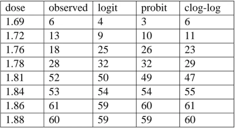
The predicted distribution of the response values from the three different link functions is listed in Table 5.3 for the “Adult Beetle Mortality” data distribution.

(24)

dose observed logit probit clog-log 1.69 6 4 3 6 1.72 13 9 10 11 1.76 18 25 26 23 1.78 28 32 32 29 1.81 52 50 49 47 1.84 53 54 54 55 1.86 61 59 60 61 1.88 60 59 59 60

Table 5.3 Predict values for Adult Beetle Mortality data

Among these three link functions, the clog-log link fits the data well, while the logit link and probit link seem like have a respectively poor fit. The logit link and probit link tend to underestimate the predict probability at the left tail. This might be expected given the asymmetry in the data and the right-skew of the distribution implied by the inverse complementary log-log link.

The information indexes, BIC and AIC, are listed in Table 5.4.

Adult Beetle Mortality

Link function

logit probit clog-log

BIC 387.2237 386.2318 379.2184

AIC 378.8719 377.88 370.8667

Table 5.4 Information indexes for Adult Beetle Mortality models

The complementary log-log link has the smallest BIC and AIC, therefore this link function seems to be the best one for these data.

(25)

5.2LINK COMPARISONS USING POSTERIOR PREDICTIVE DISTRIBUTION CHECKS

5.2.1 Model formulation and WinBUGS code

WinBUGS (the MS Windows operating system version of BUGS: Bayesian Analysis Using Gibbs Sampling) is a versatile package that has been designed to carry out Markov Chain Monte Carlo (MCMC) computations for a wide variety of Bayesian model. In this article we use WinBUGS to do model comparisons[9]_.

WinBUGS implements various MCMC algorithms to generate simulated observations from the posterior distribution of the unknown quantities (parameters or nodes) in the statistical model. The idea is that with sufficiently many simulated observations, it is possible to get an accurate picture of the distribution.

To calculate a posterior distribution it is necessary to tell WinBUGS what prior distribution to use and what likelihood distribution to use.

For the datasets introduced, the outcome variables follow a binomial distribution with mean equal to the inverse-logit of , thus, the logit transformation of is the linear predictor of the conditional mean response . We can express the likelihood in WinBUGS using the following syntax:

for(i in 1:481){

kill[i]~dbern(theta[i])

logit(theta[i]) <- beta[1]+beta[2]*dose[i] }

For the probit and complementary log-log models, the mean (inverse links) will be expressed as follows:

theta[i] <- 1-exp(-exp(beta[1]+beta[2]*dose[i] theta[i] <- phi(beta[1]+beta[2]*dose[i])

(26)

The main purpose of this report is to compare different link functions. Because there is no prior information for the regression coefficient vector β, I used diffuse priors which allow the parameters have equal probability for each possible value.

for(j in 1:2){

beta[j] ~ dnorm(0, 1.0E-4) }

After 10,000 iterations, we will get posterior distribution for each parameter. By applying a draw from a Bernoulli distribution with a posterior mean of , we can get a replicate y.

kill.rep[i]~dbern(theta[i])

Calculation of the -type statistic within WinBUGS can be done by defining the nodes sumT_obs and sumT_rep, which will calculate ( ₎_and ₍ ₎_for each iteration t of the MCMC algorithm..

for (i in 1:418) {

## expected value for each data point expect[i] <-theta[i]

## variance for each data point

variance[i] <- theta[i]*(1-theata[i]

T_rep[i] <- pow(kill.rep[i] - expect[i], 2)/variance[i] }

Referring to formula (3.4), T_rep is | _| , by adding up T_rep, we get

_{for one iteration. Using similar syntax, we will get} _{. A corresponding} posterior p-value must be also monitored as well. The posterior p-value is given by the posterior mean of the node p.chisq defined by

(27)

Here the step function will return 1 if sumT-rep is larger than sumT_obs and 0 otherwise. So by monitoring this node, we will get the posterior p-value. A p-value close to zero indicates a model with poor fit since the observed statistic will be away from what is expected under the assumed model.The complete WinBUGS code is shown in the Appendix.

5.2.2 Results

Posterior summary for the p-value from 10,000 MCMC iterations with a 5,000 iteration burn-in, I get the results shown in Table 5.5.

Link function

p-value logit probit clog-log

Age of Menarche 0.4325 0.5516 0.6013

Adult Beetle Mortality 0.4893 0.5842 0.5033

Table 5.5 Posterior summary for p.chisq

From the table above, we can see p.chisq for the logit link and probit link are closer to 0.50 than for the complementary log-log link, so those two link functions provide better fit than the complementary log-log link function for the “Age of Menarche” data. For the “Adult Beetle Mortality” data, the complementary log-log link provides a better fit than the logit or probit links

5.3LINK COMPARISON VIA ROC ANALYSIS

The “Age of Menarche” data, all three link functions produce the same sensitivity, specificity and accuracy values, which are 92.59%, 87.76% and 90.61%, respectively. For the “Adult Beetle Mortality” data, all three link functions produce the same sensitivity, specificity and accuracy values, which are 87.29%, 75.79% and 82.74%, respectively. Sensitivity, which calculated by (3.9), is the probability of getting a 1 in a

(28)

replicate y given the observed y equals 1. It’s also called true positive rate (TPR). Specificity which is calculated by (3.10), is the probability of getting a 0 in a replicate y given the observed y equals to 0. It’s also called the true negative rate TNR). We get accuracy by calculating the probability of true positive and true negative (3.11).

In general, a model with better decision performance is indicated by an ROC curve that is higher and to the left in the ROC space, which means a high sensitivity versus a low specificity that contribute a high accuracy.

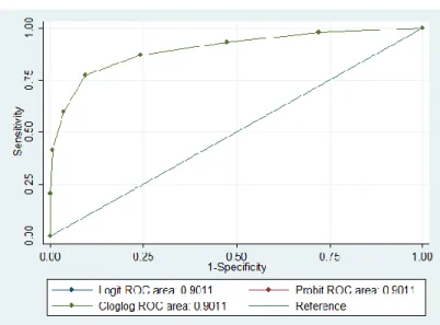
All the three links produce identical ROC curves, and the chi-square test also shows there is no significant difference within these link functions (see Figure 5.1, Figure 5.2, Table 5.6 and Table 5.7 for details).

(29)

Table 5.6Age of Menarche

Figure 5.2 ROC for Adult Beetle Mortality

Table 5.7Adult Beetle Mortality

As shown above, sensitivity, specificity and accuracy are all calculated with the summary data, it ignored accuracy for individual x level. For example, in “Adult Beetle

chi2(0) = 0.00 Prob>chi2 = . Ho: area(Logit) = area(Probit) = area(Cloglog)

Cloglog 3918 0.9721 0.0021 0.96805 0.97621 Probit 3918 0.9721 0.0021 0.96805 0.97621 Logit 3918 0.9721 0.0021 0.96805 0.97621 Obs Area Std. Err. [95% Conf. Interval] ROC Asymptotic Normal . roccomp obs Logit Probit Cloglog [fweight=freq], graph summary

chi2(0) = 0.00 Prob>chi2 = . Ho: area(Logit) = area(Probit) = area(Cloglog)

Cloglog 481 0.9011 0.0135 0.87454 0.92763 Probit 481 0.9011 0.0135 0.87454 0.92763 Logit 481 0.9011 0.0135 0.87454 0.92763 Obs Area Std. Err. [95% Conf. Interval] ROC Asymptotic Normal

(30)

Mortality” data, we observed 291 killed in total of 8 levels of dosage, the predicted killed from three links are 292, 293 and 292 respectively. There seems to be no significant difference in prediction with these link functions.

5.4CONCLUSIONS REGARDING MODEL COMPARISON METHODS

I used three model comparison methods. The information criterion index is the most efficient way to compare link functions. They are easy to get by using a single command in Stata [10]_{, and the model selected by them predicts best for the dataset.}

Also, we can use posterior predictive distribution via a Bayesian approach, but the p-value we get is similar and hard to compare, making it difficult to select the preferred link for the data. However, the calculation for the test statistic is very tedious.

The ROC analysis is not suitable for link comparison. Since ROC analysis compares the total number of success and failures predicted with total number observed, the poor fit in a signal level usually counteracts with each other. From Table 5.3, we can see in the “Adult Beetles Mortality” data, the predicted total number killed under all three links are almost identical, while the logit and probit links tend to under-estimate the number killed in the two tails and over-estimate in the middle, That is the reason why we got exactly same ROC curve for three link functions in both datasets.

(31)

6. Other Transformations for Binary Response Data

The preceding analysis shows that for different datasets, we may need to choose different link functions to provide optimal fit. The binary response datasets fall mainly into two classes, one is symmetric and the other is asymmetric. Here, symmetric means that successes and failures are interchangeable. In other words, if we code 1 as failure and 0 as success, we can get the same answer as when we code 1 as success and 0 as failure, except for opposite signs of the effects of covariates. Arando-Ordaz (1981)[11] _mentions

two families of transformations for binary response data, one is the symmetric family and the other one is the asymmetric family.

6.1SYMMETRIC TRANSFORMATION

The symmetric transformation family is given by

, (6.1)

where denotes the probability of success, denotes the transformation parameter. Since treats successes and failures in a symmetrical way, this implies that and .

When , is a logistic transformation, and when , it is linear transformation.

6.2ASYMMETRIC TRANSFORMATION

The asymmetric transformation family is defined by

{ _}_(6.2) We assume that , where has a linear expression . For , it is the complementary log-log transformation.

(32)

6.3CONCLUSION

By choosing a different value for the transformation parameter, we can find the best link for the data, or we can use the data to choose a link function.

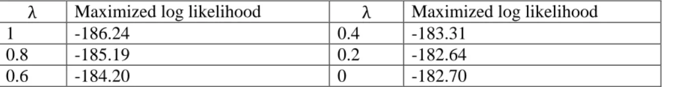
Arando-Ordaz (1981) tests a set of transformation parameters for asymmetric model using the “Adult Beetle Mortality” data, the results are shown in Table 6.1.

Maximized log likelihood Maximized log likelihood

1 -186.24 0.4 -183.31

0.8 -185.19 0.2 -182.64

0.6 -184.20 0 -182.70

Table 6.1 Maximized log likelihood for several values of

While , which conforms to a complementary log-log link fits the data pretty well, is the best one.

Although the link function can be chosen from a set of transformation parameters, the differences between these choices are very small. As the example shows above, the best choice seem to be , which has a log likelihood of -182.64, while is also a decent choice, which has a log likelihood of -182.70. But when , which is a complementary log-log link, the interpretation for the regression coefficients are much simpler than when .

(33)

7. Conclusion

As shown above, for the datasets I analyzed, the probit and logit link functions fit the symmetric one better, while the complementary log-log link fits the asymmetric one better.

The dot in the figure below is the observed probability and the fitted lines under three link functions are also shown. Although we can see the dots are more concentrated around the complementary log-log model for the asymmetric dataset and more concentrated around probit and logit model for the symmetric dataset, these three models provide decent fit as a whole.

Figure 7.1 Observed values verses fitted regression line

I did a small simulation in R[12]_{to compare the probit and complementary log-log}

link functions. I generated 1,000 data points from normal distribution and fit the data in to a probit and clog-log model respectively, then compared the model deviance.

(34)

The probit model yields a better fit 93% of the time. That is because the shapes of probit and complementary log-log are different. Probit is symmetric while clog-log is not. If the probability of success rises slowly from zero, but then tapers off more quickly as it approaches one, we may choose complementary log-log link.

For the two symmetric links, I did a similar simulation and got results as follows:

Even when we know the data were generated by a probit model, the probit model only yields a better fit 69% of the time. That is because the similar shape between logit and probit link. They are practically identical except that the logit is slightly further from the bounds then they turn the corner. That means they only have a slight difference in the tail. Though quantitatively the logit link function and the probit link function are very close to each other, qualitatively they differ significantly. That means that mathematically we can choose either logit or probit functions, but we still need to consider the underlying theoretical model.

(35)

ratios after transforming the model coefficients. It is easy to compute and easy to interpret.

However, for some dichotomous variables, one can argue that the dependent variable is a proxy for a variable that is really continuous. For example, if you model high blood pressure as a function of some covariates, one may assume that blood pressure itself is normally distributed in the population. Nonetheless, clinicians often dichotomize it using cut-off thresholds during a study (that is, they only record “High” or “Normal”). In this case, the probit model might be preferable a-priori for theoretical reasons.

(36)

Appendix

WinBUGS code for goodness-of-fit assessment in Bayesian analyses

model{ ## priors for(j in 1:2){

beta[j] ~ dnorm(0, 1.0E-4) p2[j] <- step(beta[j]) }

## Likelihood for(i in 1:481){

kill[i]~dbern(theta[i])

logit(theta[i]) <- beta[1]+beta[2]*dose[i] ##logit link theta[i] <- phi(beta[1]+beta[2]*dose[i]) ##probit link theta[i] <- 1-exp(-exp(beta[1]+beta[2]*dose[i]))##clog-log link

## Check model fit--Generate replicate data and compute fit statistics for them kill.rep[i]~dbern(theta[i]) ## replicate data for each data point

expect[i] <-theta[i] ## expected value for each data point

variance[i] <- theta[i]*(1-theta[i] ## variance for each data point T_rep[i] <- pow(kill.rep[i] - expect[i], 2) / variance[i]

T_obs[i] <- pow(kill[i] - expect[i], 2) / variance[i] } sumT_rep <- sum(T_rep[]) ## Chi-square of replicated data sumT_obs <- sum(T_obs[]) ## Chi-square of observed data

p.chisq <- step(sumT_rep-sumT_obs ## p-value for chi-square discrepancy }

(37)

References

1. Nelder, J. A. and Wedderburn, R. W. M. (1972). Generalized linear models. J.R. Statist. Soc. A, 135, 370-384.

2. P. McCullagh and J. A. Nelder. (1989). Generalized linear models. Chapman and Hall, London, 2nd Edition.

3. C. Czado and T. J. Santner. (1992). The effect of link misspecification on binary regression inference. Journal of Statistical Planning and Inference, 3, 213-231. 4. Raftery, A. E. (1976). Approximate Bayes factors and accounting for model

uncertainty in generalized linear model. Biometrika, 83, 251-266.

5. Press, S. J. (1989). Bayesian Statistics: Principles, Models, and Applications. John Wiley and Sons, Inc., New York.

6. Metz, Charles E. (1978). Basic Principles of ROC Analysis. Seminars in Nuclear Medicine, VIII(4), 284-298.

7. Milicer, H. and Szczotka, F. (1966). Age at Menarche in Warsaw Girls in 1965. Human Biology, 38(3), 199-203.

8. Bliss, C. I. (1935). The Calculation of the Dosage-Mortality Curve. Annals of Applied Biology, 22, 134-167.

9. Lunn, D.J., Thomas, A., Best, N., and Spiegelhalter, D. (2000) WinBUGS -- a Bayesian modelling framework: concepts, structure, and extensibility. Statistics and Computing, 10:325--337.

10. StataCorp. 2013. Stata Statistical Software: Release 13. College Station, TX: StataCorp LP.

11. Arando-Ordaz, Francisco J. (1981). On Two Families of Transformations to Additivity for Binary Response Data. Biometrika, 68, 357-363.

12. R Core Team (2013). R: A language and environment for statistical computing. R Foundation for Statistical Computing, Vienna, Austria. URL http://www.R-project.org/.