Simulation Study of ECCD by GNET with Momentum Conserving
Collisional Operator
∗
)
Soichiro HASEGAWA, Sadayoshi MURAKAMI and Yohei MORIYA
Department of Nuclear Engineering, Kyoto University, Nishikyo, Kyoto 615-8530, Japan (Received 9 December 2012/Accepted 26 April 2013)
The conservation of the momentum during particle collisions is important for studying the electron cyclotron current drive (ECCD). Two momentum conserving collision models are considered applying an iterative method and implemented to GNET code, in which the drift kinetic equation for energetic electrons are solved in 5-D phase space. The simulation results show a good conservation of the momentum and the calculated ECCD current is larger than the non-conserving one.
c
2013 The Japan Society of Plasma Science and Nuclear Fusion Research
Keywords: ECH, ECCD, Heliotron J, Fisch-Boozer effect, Ohkawa effect DOI: 10.1585/pfr.8.2403083
1. Introduction
Electron Cyclotron Current Drive (ECCD) is a reli-able methods to drive a plasma current by injecting the electron cyclotron wave. The electron cyclotron wave is in the GHz frequency range and the wave absorption po-sition can be controlled locally by changing the magnetic field strength. Consequently, ECCD can control current profile locally and has been applied for toroidal devices to keep the current profile, to stabilize MHD instabilities and to cancel the bootstrap current in helical systems.
In order to study the physics of ECCDs, we have simulated the current drive by Electron Cyclotron Heating (ECH) on the Heliotron J device using the GNET code [1]. GNET solves the drift kinetic equation for energetic parti-cles in 5D phase space. It has been developed for transport study of high energy electrons in helical systems and has been applied to ECCD analysis in helical systems.
In a previous study [2], we simulated the current drive in the Heliotron J and found qualitative agreement be-tween numerical simulation and experimental measure-ment. There are two well known ECCD mechanisms: (1) the Fisch–Boozer effect; and (2) the Ohkawa effect [3]. These effects drive the current in opposite directions. The result implies that EC current is driven by the Fisch– Boozer effect and Ohkawa effect.
In the present GNET code, the linear Monte Carlo lision operator is applied. This operator expresses the col-lisional effect between test particle and background par-ticle only as the pitch angle scattering and energy slow down. This operator does not express the change for the background paricle distribution and ignore the momen-tum transferred from the test particle to the background. It is pointed out that conserving momentum in electron-author’s e-mail: [email protected]
∗)This article is based on the presentation at the 22nd International Toki
Conference (ITC22).
electron collisions may have the effect for the current [4], it is necessary to modify the operator to conserve momen-tum. The Ray tracing code show a large impact of par-allel momentum conservation for ECCD simulation [5, 6]. However, in the previous study the finite orbit and radial drift effects are not considered because of a radially local assumption.
In the study presented here, in order to study ECCD quantitatively, we develop collisional operators conserving momentum for GNET. Splitting the collisional operator into two parts, we can consider the test particle’s momen-tum given to the background one. Two momenmomen-tum con-serving collision operator models are considered applying an iterative method and implemented to GNET code. We simulate the ECCD in the Heliotron J plasma with the mo-mentum conserving operators. The results show a good conservation of the momentum and the calculated ECCD current is larger than the non-conserving one.
2. Simulation Model
The GNET code can solve the linearized drift kinetic equation as a (time–dependent) initial value problem based on the Monte Carlo technique in 5D phase space. A tech-nique similar to the adjoint equation for dynamic linearized problems is used and the linearized drift kinetic equation for the deviation from the Maxwellian background,δf, is solved. We can obtain the steady state solution of the dis-tribution function by GNET. In helical system the motion of trapped particles becomes complicated because of the complex 3D magnetic configuration. Therefore, in order to analyze ECH in detail on helical systems, we have to take into account of the radial diffusion of trapped parti-cles. Thus, we must consider the distribution function at least in 5D phase space.
In GNET the gyrophase averaged electron distribution
c
2013 The Japan Society of Plasma
function is described as
f(x,v,v⊥,t)= fmax(r,v2)+δf(x,v,v⊥,t), (1)
where fmax(r,v2) represents a Maxwellian depending on
the effective radiusr. The linearized drift kinetic equation can be written with the initial condition δf(x,v,v⊥,t = 0)=0 as
∂δf
∂t +(vd+v)· ∂δf
∂x +v˙· ∂δf
∂v
=Ccoll(δf)+Lorbit(δf)+Sql(fmax), (2)
wherevd is the drift velocity andv(=vb) is the parallelˆ
velocity. The acceleration term ˙v=v˙+v˙⊥is given by the conservation of magnetic moment and total energy. Ccoll
andLorbit are the collision operator and the particle loss
term respectively. Sql represents the quasi-linear heating
term.
We assumed theSqlas
Sql = 1 v⊥
∂ ∂v⊥
⎡ ⎢⎢⎢⎢⎢ ⎣v⊥Drf
v⊥ vthe 2 ×δ
ω−2ωce
γ −kv
∂ ∂v⊥fmax
, (3)
where Drf is the wave diffusion coeficient and vthe = √
2Te/meis the electron thermal velocityωandωceare the
EC wave frequency and the electron cyclotron frequency, respectivelyk = ωn/c is the prallel component of the wave vector andγ=(1−v2/c2)−1/2is the Lorentz factor.
The delta function in Eq. (3) is approximated by the Gaus-sian function which has the broadening factorΔ, and then, Eq. (3) is described as
Sql=−2Drf v⊥ ∂ ∂v⊥ ⎡ ⎢⎢⎢⎢⎢ ⎣ v⊥ vthe 4 1 π1/2Δ
×exp⎧⎪⎪⎨⎪⎪⎩−
γ(1−kv/ω)−2ωce/ω
Δ
2⎫⎪⎪⎬
⎪⎪⎭fmax
⎤ ⎥⎥⎥⎥⎥ ⎦.
(4) The form ofSqldepends of the broading factor.
Ccoll(δf) represents the effect of collision between test
particles and background patricles. In previous study, we approximated the term as linearlized collision operator and the particle collision by the s-species (electron and ions) were given by
Ccolls (δf) ∼ C(δf,fmax)
= 1
v ∂ ∂v
v2ν2E
vδf +Ts m ∂δf ∂v +ν s d 2 ∂
∂λ(1−λ2) ∂δf
∂λ , (5)
whereC(δf,fmax) is test particle operator which represents
the collisional effect for the test particle, λ = v/v, and ν2
E andνsd are the energy transfer rate and the deflection
collision frequency by a background of s-species particles, respectively.
In order to conserve the momentum, we assume the particle collision term as
Ccoll(δf)=C(δf,fmax)+C(fmax, δf), (6)
whereC(fmax, δf) is the field particle operator which
rep-resents the collision effect for the background particles. In this study we consider two models. One is very easy to implement but it does not include the information in the velocity space. We named it as the “simple” model. The other includes all information in the velocity space, but it is now being implemented. We named it as “velocity de-pendent” model.
In the simple model, we assume a high speed limit and C(f) is expressed as
C(fmax, δf)=p(x,v)fmax, (7)
wherep(x,v) is a function of the real space coordinatex and the velocityv. p(x,v) is determined by calculating the conservation low of the energy and momentum. After some calculations, we obtain
p(x,v)=v·p(x)+λ(x) ⎛ ⎜⎜⎜⎜⎝v2
v2 the
−3
2 ⎞
⎟⎟⎟⎟⎠, (8)
where
p(x)=− 2 n0v2the
vC(δf,fmax)dv, (9)
λ(x)=− 2
3n0v2the
v2C(δf,fmax)dv, (10)
where n0 means the density of background electrons.
Once p(x,v) is obtained from Eq. (8), we can calculate C(fmax, δf) which compensates the lost momentum and
en-ergy from test particle. Then we can considerC(fmax, δf)
as a new source–sink term.
In the GNET code, if we iteratively calculate untilδf converges, we obtain a final profile ofC(fmax, δf). We
la-bel the steady state solution obtained by usingSql asδf 0
and useC(fmax, δf0) which becomes a new source term.
The steady state solution of this source term isδf1.
Obtain-ingδf1, we can consider the conservation of momentum
when we calculateδf0. However the test particle lost the
momentum due to the collision with background plasma in the process of calculatingδf1. Therefore we iteratively
calculateδfn(nis the natural number) as ∂δf0
∂t +(vd+v)·∂δ
f0
∂x +v˙· ∂δf0
∂v −C(δf0,fmax)
=Sql(fmax)+Lorbit(δf), (11)
∂δf1
∂t +(vd+v)·∂δ∂xf1 +v˙·∂δ∂vf1 −C(δf1,fmax)
=C(fmax, δf0)+Lorbit(δf),
...,
particle lost and calculate the momentum loss rate from them. We stop the iteration when the momentum loss rate becomes small sufficiently. After the iterative method, we obtain the conserving momentum distribution function by calculatingniδfi.
3. Simulation Result
In this study we consider the magnetic configuration, heating and plasma parameters as the previous paper [2]. Various magnetic configurations are capable in Heliotron J device by changing the ratio of coil currents. Here we con-sider bumpiness b, which is the parameter characterizing
magnetic configurations given by
b=B04/B00, (12)
whereBmn represents the Fourier component of the mag-netic field strength in Boozer coordinates, and m and n are the poloidal and toroidal mode numbers, respectively. We assume the configuration b = 0.01 at the magnetic
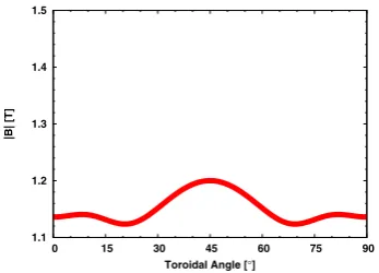
flux surface ρ = 0.67. The radial heating point is set to (ρ0, φ0, θ0) = (0.1,45◦,0◦). We also set the
parame-ters describing the EC resonance condition as follows: EC wave frequency is 70 GHz, 2ωce/ω=0.98,n =0.44 and
Δ =1.0×10⁻³. Figure 1 shows the magnetic field strength
along the magnetic axis. Fixing the toroidal angle of heat-ing point asφ0 =45◦, EC power is deposited at the top of
the ripple in this configuration.
We run the GNET iteratively and obtain the steady state solution,δf. Figure 2 (a) shows the firstly obtained distribution function. The distribution becomes asymmet-ric inv at the high energy region. This is because many ECRH accelerated electrons hardly become trapped and the collisional relaxtion of the electron deficit in low en-ergy region is faster than that of the accelerated electrons. As a result, the excess of electrons with positivevoccured and it is found that the negative toroidal current is driven by the Fisch-Boozer effect. Figure 2 (b) shows the source– sink term to conserve the momentum using the steady state solutionδf0. Then the steady state solutionδf1 is
evalu-ated using the this source–sink term (Fig. 2 (c)) and again the next source–sink term is evaluated (Fig. 2 (d)). In the two source–sink terms we can see the larger distribution in
Fig. 1 The magnetic field strength along the magnetic axis.
the positivev region and this means the lost momentum have large effect in this region.
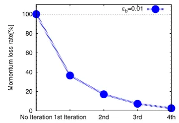
Figure 3 shows the momentum loss rate at the each iterative calculation in the simple model. We evaluate the momentum loss at each calculation, and define the momen-tum loss rate as ploss = (p0 −pn)/(p0), where p0 is the
momentum lost by test particle at first calculation and pn represents one at then th iterative caluculation. Figure 3 shows the momentum loss decreases as the iterative calcu-lation advanced and dropped less than 5% of lost momen-tum than initial simulation. The calculated ECCD current of the simple model is−20.1 kA and the non-conserving one is−18.4 kA. We can see the calculated ECCD current
Fig. 2 Flux averaged distribution function of (a)δf0, (b) source–
sink termC(fmax, δf0), (c)δf1 and (d) source–sink term
C(fmax, δf1). Increase (δf+) and decrease (δf−) area from
the Maxwellian are colored with red and blue, respec-tively. These results are calculated inne=0.5×10¹⁹m−3,
Te=1.0 keV, whereneis electron density andTeis
Fig. 3 The momentum loss rate at each iterative calculation.
is larger by 9.2% than that of non-conserving one.
4. Development of Velocity Dependent
Model
Though the simple model conserves the momentum, it does not include the exact information in the velocity space. Therefore it is necessary to implement the more ex-act model. The velocity dependent model is derived from the Fokker–Planck collisional term directly, so it includes exact information more than the simple one.
The field particle operator can be expressed using Legendre polynominalsPn(cosθ) as
C(fmax, δf)= ∞
n=0
Cn(fmax, δf(n)(v))Pn(cosθ), (13)
wherevis the total velocity of an electron andθrepresents the pitch angle. Introducing the Trubnikov-Rosenbluth po-tential and defineu =cosθto simplfy [7, 8], we can de-scribe field particle termCn(fmax, δf(n)(v)) as
Cn(fmax, δf(n)(ve))= Λe/efmax ∞
i=0 Pi(ve)
δf(n)(ve) (14)
+2 ve
0
u2δf(n)(u)
n+u i+2
vi+1 e
−n− u i
vi−1 e
− 1
2i+1 ui vi+1
e
du
+2
∞
ve
u2δf(n)(u)
n+v i+2 e
ui+1 −n− vie ui−1
− 1
2i+1 vie ui+1
du
,
wheren+ = (i +1)(i+2)/(2i +1)(2i +3), n− = (i − 1)i/(2i−1)(2i+1), ve = v/vthe. Λe/erepresents the
am-plitude of field particle term and in this paper it is assumed asΛce4/m2e 02, whereΛcis coulomb logarithm,eis charge,
meis mass of an electron and 0is permittivity in vacuume.
In order to obtain the field particle termCn(fmax, δf(n)(v))
which is determined by the obtained pertubed distribution functionδf(n)(v). We can iteratively calculateδf(n)(v) in
the same way with the simple model case. After the iter-ative method, we calculate the complete collision operator according to Eqs. (6) and (13).
Figure 4 shows the first two distribution functions and field particle terms in this procedure. The firstly obtained distribution function generates the first field particle term C0(fmax, δf(0)(v)) (Fig. 4 (a)). Then the second distribution
Fig. 4 Flux averaged distribution function of (a) field particle termC0(fmax, δf(0)(v)), (b)δf(1)and (c) field particle term
C1(fmax, δf(1)(v)).
function (Fig. 4 (b)) is calculated from the field particle term and the cycle is repeated (Fig. 4 (c)).
The velocity dependent model (Fig. 4) shows the quli-tatively similar result in the velocity space. The field parti-cle terms (Figs. 4 (a), (c)), which correspond to the source– sink term in the simple model, show the distribution func-tion will be increased at negativev area in high energy region. The steady state solution of field particle term (Fig. 4 (c)) shows the distribution function is increased at positive v area, and it means the lost momentum have large effects in this area. The velocity dependent model gives the more exact information in the velocity space, but we have not yet finished implementing this model to GNET.
5. Conclusion
models. It is easy to implement the simple model and we obtained ECCD current with the momentum conserving. However it does not include the exact information in the velocity space. Therefore we are implementing the veloc-ity dependent model which is expected to include the exact information in the velocity space.
Acknowledgement
The authors would appreciate the useful comments of-fered by Dr. Raburn for improving our paper. This work is supported by Grant-in-Aid for Scientific Research (C)
(23561000) and (S) (20226017) from JSPS, Japan.
[1] S. Murakamiet al., Nucl. Fusion40, 693 (2000). [2] Y. Moriyaet al., Plasma Fusion Res.6, 2403139 (2011). [3] R. Prater, Phys. Plasmas11, 2349 (2004).
[4] R. Prateret al., Nucl. Fusion48, 035006 (2008). [5] H. Maaßberget al., Phys. Plasmas19, 102501 (2012). [6] N.B. Marushchenko et al., Phys. Plasmas 18, 032501
(2011).
[7] M.N. Rosenbluthet al., Phys. Rev.107, 1 (1957). [8] M. Brambilla,Kinetic Theory of Plasma Waves