Meshless Time-Domain Method with Modified RPIM-Based Shape
Functions for Electromagnetic Wave Propagation Simulation in
Complex Shaped Domain
∗
)
Taku ITOH, Soichiro IKUNO and Hiroaki NAKAMURA
1)Tokyo University of Technology, 1404-1 Katakura-machi, Hachioji, Tokyo 192-0982, Japan
1)National Institute for Fusion Science, 322-6 Oroshi-cho, Toki, Gifu 509-5292, Japan
(Received 10 December 2013/Accepted 27 March 2014)
To speed up electromagnetic wave propagation simulations using the meshless time-domain method (MTDM) in complex shaped domains, this paper presents a strategy for embedding the modified ra-dial point interpolation method (MRPIM)-based shape functions to MTDM, while maintaining the stability of the simulations. Numerical experiments show that, by using the strategy with appropriate parameters, the sta-bility of the simulations using MTDM with MRPIM-based shape functions (MRPIM-MTDM) is considerably improved. In addition, the approach of the amplification/damping rate to convergence in MRPIM-MTDM is al-most the same as that in the conventional MTDM. Furthermore, the total computation time of MRPIM-MTDM is less than that of the conventional MTDM.
c
2014 The Japan Society of Plasma Science and Nuclear Fusion Research
Keywords: meshless time-domain method, meshless radial point interpolation method, electromagnetic propa-gation, waveguide bend, Maxwell equation
DOI: 10.1585/pfr.9.3401088
1. Introduction
In a large helical device (LHD), an electron cyclotron heating (ECH) system is used for plasma heating; electri-cal power generated by the gyrotron system is transmitted to the LHD via a long corrugated waveguide. However, the shape of the waveguide curvature and the theoretical trans-mission gain of electromagnetic wave propagation are not clear [1].
Finite-difference time-domain method (FDTD) has generally been applied to electromagnetic wave propaga-tion simulapropaga-tions. FDTD can directly provide solupropaga-tions of Maxwell equations. However, to apply FDTD in electro-magnetic wave propagation simulations, the numerical do-main must be divided into rectangular meshes, and it is difficult for an arbitrary-shaped domain to be accurately represented by rectangular meshes.
On the other hand, a meshless method based on the radial point interpolation method (RPIM) [3] has recently been applied to electromagnetic wave propagation simu-lations [2]. We refer to this as a meshless time-domain method (MTDM). MTDM does not require finite ele-ments or meshes of a geometric structure, i.e., the node alignment of MTDM is more flexible than that of FDTD. Hence, MTDM can easily be applied in electromagnetic wave propagation simulations of complex shaped domains. However, the computational cost of MTDM tends to be larger than that of FDTD. This is because, in MTDM,
author’s e-mail: [email protected]
∗)This article is based on the presentation at the 23rd International Toki
Conference (ITC23).
shape functions based on RPIM are usually employed; i.e., before starting the simulations, theith shape function cor-responding to theith node has to be determined by solv-ing linear systems constructed by ussolv-ing neighbor nodes (i=1,2, . . . ,N), whereNis the number of nodes. To apply MTDM to large-scale simulations, acceleration of MTDM may be indispensable.
Recently, a modified RPIM (MRPIM) [4] has been proposed. In MRPIM, the algorithm for determining the shape functions is rebuilt. By using MRPIM-based shape functions in MTDM, the computation efficiency of MTDM may be improved. However, if MRPIM-based shape func-tions are simply embedded in MTDM, the simulation using MTDM may be unstable [1].
The purpose of the present study is to speed up elec-tromagnetic wave propagation simulations using MTDM in complex shaped domains. To this end, MRPIM is em-ployed for generating shape functions for MTDM. In addi-tion, to maintain the stability of simulations using MTDM, we present a strategy for embedding MRPIM-based shape functions in MTDM.
2. Meshless Time-Domain Method
To simulate electromagnetic wave propagation, we consider Maxwell equations in case of the two-dimensional (2D) TM mode described byε∂Ez
∂t =−σEz+
∂Hy
∂x −
∂Hx
∂y , (1)
c
2014 The Japan Society of Plasma
μ∂Hx
∂t =−
∂Ez
∂y , (2)
μ∂Hy
∂t =
∂Ez
∂x , (3)
whereEzdenotes thezcomponent of the electric field, and
HxandHydenote thexandycomponents of the magnetic
field, respectively. In addition,ε, σ, andμdenote the per-mittivity, electrical conductivity, and the magnetic perme-ability, respectively.
To discretize (1)–(3) by MTDM, nodes xE i (i =
1,2, . . . ,NE) forEzandxHi (i = 1,2, . . . ,N H
) forHxand
Hy are first aligned in a domain, where NE denotes the
number of nodes for Ez, and NH denotes the number of
nodes for Hx and Hy. In MTDM, the leapfrog method
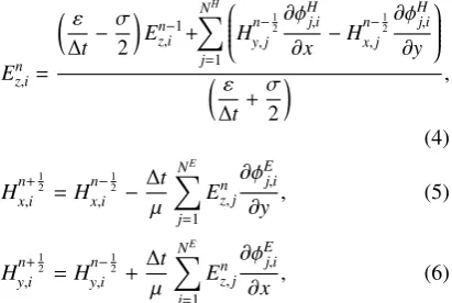
is employed to discretize the time-domain. The space domain is discretized by using shape functions based on meshless methods. The discretized forms of (1)–(3) are as follows [1, 2, 5]:
Enz,i=
ε
Δt−
σ 2
Ezn,−i1+ NH
j=1
⎛ ⎜⎜⎜⎜⎜ ⎝Hn−
1 2
y,j
∂φH j,i
∂x −H
n−1 2
x,j
∂φH j,i
∂y
⎞ ⎟⎟⎟⎟⎟ ⎠
ε
Δt+
σ 2
,
(4)
Hn+12
x,i =H n−1
2
x,i −
Δt
μ
NE
j=1
Enz,j∂φ
E j,i
∂y , (5)
Hn+
1 2
y,i =H n−1
2
y,i +
Δt
μ
NE
j=1
Enz,j
∂φE j,i
∂x , (6)
wherenis the time step,En z,i≡E
n z(xEi),H
n+1 2
x,i ≡H n+1
2
x (xiH),
and Hn+
1 2
y,i ≡ H n+1
2
y (xHi ). In addition, φ E
j(x) and φ H
j(x)
denote the shape functions corresponding to xE j (j =
1,2, . . . ,NE) andxHj (j=1,2, . . . ,N H
), respectively.
3. Shape Functions for MTDM
By using MTDM, Ez,Hx, andHyin (1)–(3) are
dis-cretized by shape functions based on meshless methods. Note that the shape functionsφEj(x) andφHj(x) in (4)–(6) are similarly determined. Hence, in this section, we do not useEandHas superscripts.
In MTDM, it is assumed that the shape functions sat-isfy a property, φi(xj) = δi j, whereδi j is the Kronecker
delta [3]. In the following section, we describe the origi-nal and modified RPIM-based shape functions, since both shape functions satisfy the above property.
3.1
Original RPIM-based shape functions
First, the nodes, x1,x2, . . . ,xN, together with the
ra-dial basis functions (RBFs), w1(x),w2(x), . . . ,wN(x), on
each of the nodes are assigned in the domainΩ and on the boundary ∂Ω, where N is the number of nodes, and
wi(x) ≡ w(|x−xi|) (i = 1,2, . . . ,N). In RPIM, it is
as-sumed that a functionu(x) can be expanded as
Fig. 1 Support domains for (a) original RPIM-based shape func-tion and (b) modified RPIM-based shape funcfunc-tion.
u(x)=
N
i=1
uiφi(x), (7)
whereuiis a coefficient, andφi(x) denotes the shape
func-tion corresponding to theith nodexi(i=1,2, . . . ,N). Note
that theith shape function is defined by using a support do-main centered at an observation point x. A schematic of the rectangular support domain is illustrated in Fig. 1 (a).
Inside the support domain, the shape functions φ1(x), φ2(x), . . . , φNs(x) corresponding to x1,x2, . . . ,xNs
are determined by solving the linear systems as follows [3]:
Gφ(x)=b(x), (8)
where x1,x2, . . . ,xNs are nodes contained in the support
domain,Nsis the number of nodes inside the support,
G≡
W P
PT O
, b(x)≡
w(x)
p(x)
, (9)
W ≡[w(x1),w(x2), . . . ,w(xNs)]
T,
P≡[p(x1),p(x2), . . . ,p(xM)]T,
φ(x)≡[φ1(x), φ2(x), . . . , φNs+M(x)]
T,
w(x)≡[w1(x),w2(x), . . . ,wNs(x)]
T, and
p(x)≡[p1(x),p2(x), . . . ,pM(x)]T.
Similarly, partial derivatives ofφ(x) with respect toxandy
are, respectively, determined by solving the linear systems as follows:
G∂φ
∂x(x)=
∂b
∂x(x), andG
∂φ ∂y(x)=
∂b
∂y(x). (10)
In this study, for the 2D case, we adopt M = 3; i.e.,
p(x) = [1,x,y]T, whose components are coefficients of a
3.2
Modified RPIM-based shape functions
In MRPIM, the coefficient matrixGin (8) and (10) is independent of the observation point x; instead, G is constructed for each subdomain. Figure 1 (b) shows an example of rectangular subdomainsΩ1, Ω2, . . . , Ωm
gener-ated by dividing the domainΩ. This figure also shows a support domainΩi for theith subdomainΩi. Note thatΩi
is not determined from the observation pointxbut from the center ofΩi[4].
4. Strategy for Embedding
MRPIM-Based Shape Functions in MTDM
In MRPIM, the subdomains,Ω1, Ω2, . . . , Ωmand their
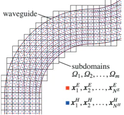
support domains have to be determined. For electro-magnetic wave propagation simulations by MTDM with MRPIM-based shape functions in waveguide bends, we choose rectangular subdomains of the same size, since we suppose that nodes xE
i (i = 1,2, . . . ,N
E) and xH i (i =
1,2, . . . ,NH) are uniformly aligned inside the waveguide. Figure 2 shows a schematic of the rectangular subdomains. InΩi, to determine the support domainΩi, we present
a strategy for adjusting the numberNsof nodes contained
inΩiso thatNs∈[Nmin,Nmax] is satisfied as much as
pos-sible. Here, Nmin andNmax are user-specified parameters
that denote the minimum and maximum numbers of nodes contained inΩi. This is because ifΩidoes not contain suf-ficient nodes, unexpected evaluation results for shape func-tions may be obtained on an observation pointxinΩi. In
addition,Nsinfluences the size of the matrixG, i.e., ifNs
is too large, the computational cost for solving (8) and (10) significantly increases. Furthermore, without the strategy, simulations using MTDM with MRPIM-based shape func-tions may be unstable, as shown in Section 5. The strategy is represented by the following C-like pseudo-code that is based on an algorithm given in [6].
dx=βxlx; dy=βyly; k=0;
do{
Xs=searchNeighborNodes(Ns,c,dx,dy);
if(Ns<Nmin){dx+=βExlx; dy+=βEyly; }
else if(Ns>Nmax){dx−=βxRlx; dy−=βRyly; }
++k;
}while(Ns[Nmin,Nmax] && k<kmax);
Here,dxanddydenote the x- andy-length ofΩi,
respec-tively, andlxandlydenote thex- andy-length ofΩi,
respec-tively. In addition,βx,βy,βEx,βyE,βRx,βRy andkmaxare
user-specified parameters. In particular,βx andβy are set for
determining the initial lengths ofdxanddy, respectively;
βE
xandβEy are set for enlargingdxanddy, respectively; and
βR
xandβRy are set for reducingdxanddy, respectively. Note
thatkmaxis set for determining the maximum number of
it-erations, since satisfyingNs ∈ [Nmin,Nmax] is sometimes
difficult, depending on the node alignment.
In the function “searchNeighborNodes,” nodes con-tained in a rectangular domain ˆΩi of centerc,x-lengthdx
andy-lengthdyare searched, and the nodes are returned to
Fig. 2 Schematic of rectangular subdomains for a waveguide bend.
Xs. In addition, the numberNs of nodesXsis updated in
the function. Note that the centercof ˆΩi coincides with the center ofΩi. After the do-while loop, we setΩi =Ωˆi.
5. Numerical Experiments
In this section, numerical experiments are conducted to investigate the performance of MTDM with MRPIM-based shape functions for a 2D electromagnetic wave prop-agation simulation in the waveguide bend illustrated in Fig. 3 (a). In the figure, we setw = 0.3 m, h = 1.2 m,
andR = 0.45 m. In addition, in the simulation, we
as-sume that the wave source is a sine wave whose am-plitude, frequency, and speed are 1.0 V/m, 1.0×10⁹Hz, and 299792458 m/s, respectively. Furthermore, to sat-isfy the Courant condition for the 2D MTDM [5],Δt =
0.6 min|xH i −x
H
j|/cs (i,j=1,2, . . . ,N
H,i j), wherecis
the speed of light. In Fig. 3 (a),xE
i andx H
j are represented as red squares
and blue triangles, respectively (i = 1,2, . . . ,NE, j =
1,2, . . . ,NH). In addition, the node alignment is based on the staggered mesh that is employed in the standard FDTD. This is because the simulation may become unstable if the node alignment is inappropriate [5]. As boundary condi-tions, the perfectly matched layer (PML) and the perfect electric conductor (PEC) are employed. PMLs are im-posed at the waveguide edges, and PECs are imim-posed on the waveguide sides, as shown in Fig. 3 (a). Note that these boundary conditions in MTDM can be imposed in the same manner as in FDTD (see [7] for more details).
To generate shape functions for MTDM, we adopt a reciprocal multi quadric (RMQ):
wi(x)=
⎛ ⎜⎜⎜⎜⎝|x−xi|2
di2 +α
2
⎞ ⎟⎟⎟⎟⎠−1
2
, (11)
as the RBF in (9), wheredi =
d2
x+dy2, andαis an
user-specified parameter; we setα = 0.1. In addition, we set
lx = 1.3Δxm,ly = 1.3Δym,βx = βy = 3.0,βEx = βEy =
0.11,βR
x =βRy =0.07, andkmax=100.
double-Fig. 3 (a) Schematic of the waveguide bend employed in the numerical experiments. In this figure,xE i andx
H
j are represented as red
squares and blue triangles, respectively. (b) Distribution ofEz obtained from MRPIM-MTDM without the strategy for adjusting
Ns (t=54000Δt,N =96165). Black regions correspond to an inappropriate value forEz. (c) Distribution ofEz obtained from
RPIM-MTDM (t=70000Δt,N=302645). (d) Distribution ofEzobtained from MRPIM-MTDM (t=70000Δt,N=302645).
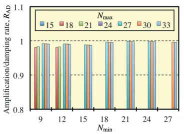
Fig. 4 Dependence of the amplification/damping rate RAD on
NminandNmaxforN=211715.
precision arithmetic. In the following, RPIM-MTDM and MRPIM-MTDM denote MTDMs with original and modi-fied RPIM-based shape functions, respectively.
Figure 3 (b) shows the distribution ofEzobtained from
MRPIM-MTDM without the strategy for adjustingNs. The
distribution is observed int=54000Δts. The parameters for determiningN are fixed atΔx= Δy = Δr =0.006 m andΔθ =π/400, thusN =96165, whereN =NE +NH.
Note thatNE and NH include the number of nodes
con-tained in PML regions, and the number of layers for each PML region is 16. The parameters for support domains are fixed atdx=1.5lxm anddy=1.5lym, i.e.,dxanddyfor all
support domains are all the same. In Fig. 3 (b), the black parts denote regions in whichEzhas inappropriate values.
These black parts appear from aroundt =50000Δts, and
Ez subsequently diverged. These results suggest that the
simulation becomes unstable whendxanddyare constant
for all support domains. Hence, a strategy for adjustingNs
is necessary for embedding MRPIM in MTDM.
To determine appropriate values for Nmin and Nmax,
the dependence of the amplification/damping rateRADon
NminandNmaxis shown in Fig. 4. The parameters are fixed
atΔx = Δy = Δr =0.004 m andΔθ= π/600, thusN =
211715. Although a pair ofNmin andNmaxfor generating
φE
i(x) (i =1,2, . . . ,N
E) andφH
j(x) (i =1,2, . . . ,N H) can
be set separately, the same pair is used for generatingφiE(x) andφH
j(x). Note that the subdomains for φ E
i(x) and for
φH
i (x) are exactly the same. However, the support domains
forφEi(x) and forφ H
i (x) are not the same, sinceφ E i(x) and
φH
j(x) are separately generated, although the same pair of
NminandNmaxis chosen. Here, the amplification/damping
rateRADis defined as follows:
RAD≡
Γ2
|E×H| d
t Γ1
|E×H| d
t
. (12)
In (12), to calculateRAD, the y-coordinate ofΓ1and that
of Γ2 are set to 0.6 and 2.4, respectively (see Figs. 3 (c)
and 3 (d)). In Fig. 4, we attempted to calculateRAD for
all cases that satisfy Nmin < Nmax. However, for some
pairs ofNminandNmax,RADcould not be calculated, since
the simulations using these pairs were unstable. Note that
RAD for these pairs are not shown in Fig. 4. Especially
for Nmax = 15 and 24, the simulations were always
un-stable. For this reason, there is no bar forNmax =15 and
24 in Fig. 4. The figure shows that, whenNminis relatively
small,RADcannot be calculated occasionally. In addition,
forNmax≥27,RADcan be calculated for all cases. Based
on these results, we fixedNmin=21 andNmin =27.
For the following, electromagnetic wave propagation is simulated by using the above fixed values forNmin and
Nmax. Figures 3 (c) and 3 (d) show distributions ofEz
ob-tained from RPIM-MTDM and MRPIM-MTDM, respec-tively. Both distributions were observed att=70000Δts. Parameters are fixed atΔx = Δy = Δr = 1/300(m) and Δθ = π/720, thus N = 302645. It must be noted here that, when MRPIM-MTDM without the strategy for ad-justing Ns is applied to a simulation with the same
pa-rameters, the simulation becomes unstable from around
t = 1400Δt. Hence, by using the strategy with appro-priate parameters, the stability of electromagnetic wave propagation simulations using the MRPIM-MTDM is con-siderably improved. For the quantitative comparisons be-tween the two distributions, a maximum error εmax ≡
maxNE
Fig. 5 Dependence of the amplification/damping rateRADonN.
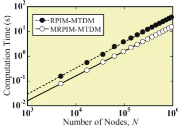
Fig. 6 Computation time dependence for determining the partial derivatives ofφE
i(x) at x H
j and those ofφ H j(x) atx
E i on
N(i=1,2, . . . ,NE, j=1,2, . . . ,NH).
εavg≡N
E
i=1|ERPIMz,i −EMRPIMz,i |/(N
Emax|E
z|) are calculated,
where ERPIM
z,i and EzMRPIM,i denote Ez(x E
i) obtained from
RPIM-MTDM and MRPIM-MTDM, respectively. In ad-dition, max|Ez| = 1.0, since the wave source is a sine
wave whose amplitude is 1.0 V/m. The calculated errors areεmax=1.72×10⁻²andεavg=1.68×10⁻³. Hence,
al-though the two distributions in Figs. 3 (c) and 3 (d) are vi-sually almost the same, the difference betweenERPIM
z,i and
EMRPIM
z,i is up to about 1.72% and on average it is about
0.168%.
To investigate the convergence ofRADin both
meth-ods,RADis plotted as a function ofN, as shown in Fig. 5.
The figure shows that there is no obvious difference be-tweenRAD of the two methods. In addition, from around
N = 100000,RAD 1.0 in both methods. In the
meth-ods, RAD essentially converged to a value that is slightly
less than 1.0. SinceRAD < 1 at convergence, the
electro-magnetic wave is slightly damped in both methods. We consider that this damping is caused by wave reflections in the waveguide bend.
Finally, we investigate the computation time of both methods. We first focus on the iteration of (4)–(6). For 30000 iterations and N = 96165, the computation times for RPIM-MTDM and MRPIM-MTDM are about 467.7 s and 410.1 s, respectively. For 30000 iterations andN =
302645, the computation times for RPIM-MTDM and MRPIM-MTDM are about 1454.3 s and 1282.6 s, respec-tively. From these results, we conclude that
MRPIM-MTDM is slightly faster than RPIM-MRPIM-MTDM. Next, we focus on the process for determining ∂φEi
∂x(x H
j),
∂φE i
∂y(x H j),
∂φH j
∂x(x E i) and
∂φH j
∂y(x E
i) (i =1,2, . . . ,N
E, j =1,2, . . . ,NH).
This process is required once before starting the iterations of (4)–(6). For both methods, the computation time de-pendence for this process on N is shown in Fig. 6. The figure shows that, in all cases, the computation time for MRPIM-MTDM is about 2.38 times less than that for RPIM-MTDM. Therefore we conclude that the total com-putation time for MRPIM-MTDM is less than that for RPIM-MTDM. Especially whenNis large, the difference in the computation times increases for the two methods.
6. Conclusion
To speed up electromagnetic wave propagation sim-ulations using the MTDM in complex shaped domains, a strategy for embedding the modified radial point interpo-lation method (MRPIM)-based shape functions in MTDM while maintaining the stability of the simulations has been presented. In numerical experiments, the performance of MRPIM-MTDM has been investigated and compared with that of MTDM with the RPIM-based shape func-tions (RPIM-MTDM). Conclusions obtained in the present study are summarized as follows:
1. By using the strategy for adjusting Ns together
with appropriate parameters, the stability of elec-tromagnetic wave propagation simulations using the MRPIM-MTDM is considerably improved.
2. The approach to convergence of RAD in
MRPIM-MTDM is almost the same as that in RPIM-MRPIM-MTDM. 3. The total computation time for MRPIM-MTDM is
less than that for RPIM-MTDM.
In a future study, details for damping the electromag-netic wave will be investigated. In addition, MRPIM-MTDM will be applied to larger-scale problems including three-dimensional cases.
Acknowledgment
This work was partially supported by JSPS KAK-ENHI Grant Number 24700053. In addition, this work was supported in part by NIFS Collaboration Research Pro-gram (NIFS13KNTS025 and NIFS13KNXN267).
[1] S. Ikuno, Y. Fujita, T. Itoh, S. Nakata, H. Nakamura and A. Kamitani, Plasma Fusion Res.7, 2406044 (2012). [2] T. Kaufmann, C. Engström, C. Fumeaux and R. Vahldieck,
IEEE Trans. Microw. Theory Tech.58, 3399 (2010). [3] J.G. Wang and G.R. Liu, Int. J. Numer. Methods Eng.54,
1623 (2002).
[4] S. Nakata, JNAIAM4, 193 (2009).
[5] T. Itoh, S. Ikuno, Y. Fujita and H. Nakamura, Plasma Fu-sion Res.8, 2401101 (2013).
[6] I. Tobor, P. Reuter and C. Schlick, WSCG12, 467 (2004). [7] S. Ikuno, Y. Fujita, T. Itoh, S. Nakata and A. Kamitani,