Integer Versus Fractional Order SEIR Deterministic and Stochastic Models of Measles

Article

Integer versus Fractional Order SEIR Deterministic

and Stochastic Models of Measles

Md Rafiul Islam1,∗ , Angela Peace1, Daniel Medina2and Tamer Oraby2

1

2

3

4

5

6

7

8

9

10

11

1 _{DepartmentofMathematicsandStatistics,TexasTechUniversity,2500Broadway,Lubbock,Texas79409;} [email protected](MR.I.);[email protected](A.P.)

2 _{SchoolofMathematicalandStatisticalSciences,TheUniversityofTexasRioGrandeValley,1201W.} UniversityDrive,Edinburg,Texas78539;[email protected](D.M.);[email protected](T.O.) * Correspondence:[email protected]

Abstract: Inthispaper,wecomparetheperformancebetweensystemsofordinaryand(Caputo) fractionaldifferentialequationsdepictingthesusceptible-exposed-infectious-recovered(SEIR)models ofdiseases. Inordertounderstandtheoriginsofbothapproachesasmean-fieldapproximations ofintegerandfractionalstochasticprocesses,weintroducethefractionaldifferentialequationsas approximationsofsometypeoffractionalnonlinearbirth–deathprocesses.Then,weexaminevalidity ofthetwoapproachesagainstempiricalcoursesofepidemics;wefitbothofthemtocasecounts ofthreemeaslesepidemicsthatoccurredduringthepre-vaccinationerainthreedifferentlocations. WhileFDEsappearmoreflexibleinfittingempiricaldata,ourODEsofferedbetterfitstotwooutof threedatasets.Importantdifferencesintransientdynamicsbetweenthesemodelingapproachesare discussed.

Keywords: fractionalSEIRstochasticmodel;Caputofractionalorderdifferentialequations;Measles; ParameterEstimation

12

1. Introduction 13

Modeling the spread of infectious diseases before the introduction of vaccines, as well as the 14

validation of these models, has been widely studied since the works of Bernoulli [1], Ross [2], Brownlee 15

[3], Greenwood and Yule [4], Kermack and McKendrick [5], Soper [6], Greenwood [7,8], M . S . Bartlett 16

[9], Bailey [10]. See also Bailey [11] and Anderson [12] for more details about the history of disease 17

modeling. Deterministic models using ordinary differential equations (ODEs) have received great 18

attention [12–16] and wide assimilation by health sciences. See Temimeet al.[17] and the references 19

therein. Other deterministic models such as difference equations are also used to model the spread of 20

diseases; for instance, see Fismanet al.[18]. However, fractional differential equations (FDEs) have 21

been used in the last decade to model the course of epidemics [19–24]. 22

Fractional differential equations are usually used to involve the memory of the process in the 23

dynamics of the systems. There is more than one type of fractional order derivative; most notably, 24

Caputo, Grünwald-Letnikov, and Riemann-Liouville [25]. Here, we study the Caputo fractional order 25

derivative. Integer order derivatives of ordinary differential equations are special cases of fractional 26

order derivatives. It was noted in more than one paper, e.g. [26], that FDEs give a better depiction of 27

the courses of epidemics and natural phenomena than ODEs. Few researchers have fitted their FDE 28

models to data [26,27], however, they lack details on justifying the goodness of fit so as to statistically 29

validate them. This motivated us to compare systems of ODEs and FDEs by fitting them to some actual 30

epidemic data. 31

Measles is a marker disease for virological, epidemiological, clinical, statistical, geographical, 32

mathematical, and humanitarian reasons [28, p.16-21]. Mathematical modeling of measles epidemics 33

dates as far as 1888 by D’Enko and then by Hamer [28, p.19]. Regularity and a large number of cases 34

of measles’ epidemics with major peaks in the pre-vaccination era (before 1964) support the choice 35

of testing models against measles data. Many other researchers formulated measles models and fit 36

them to data, as in Bjørnstadet al.[29], where a time scale of two weeks is recommended fitting the 37

number of cases, and in Yingcun Xiaet al.[30], where a model is used to examine a spatial network. 38

In this paper, we choose to use data of measles infections in the US and UK in two decades of the 39

pre-vaccination era (1944−1964), to compare the goodness of fit of ODEs and FDEs to those epidemics. 40

While ordinary differential equations are well-established as deterministic models of the spread 41

of diseases (see e.g. Greenwood and Gordillo [31] and Vasilyevaet al.[32]), FDE models are sometimes 42

used. However, often these approaches lack mathematical basis or physical interpretation except 43

for exchanging integer differentiation with fractional ones, (see e.g. Almeidaet al.[26] and Aranda 44

et al.[33]). Angstmannet al.[34] and Sardaret al.[35] provided a valid variation by considering the 45

memory of the non-Markovian infection process. The result is a mixed system of integer and fractional 46

derivatives of the Riemann-Liouville type. Saeedianet al.[36] showed how another memory functional 47

of the process can lead to replacing the integer derivatives with Caputo fractional derivatives. In this 48

paper, we show how Caputo fractional differential equations follow naturally from fractional stochastic 49

processes like those introduced in [37–46]. Then we show that for different data sets, FDE models fit 50

the data better for some epidemics whereas ODE models fit better for others. The Akaike Information 51

Criterion (AIC) and Bayesian Information Criterion (BIC) are used to compare between the fittings of 52

the two models to three data sets. For completeness, we will cover all the required background and the 53

relevant definitions in section2. That includes a synopsis of Caputo’s fractional calculus and fractional 54

stochastic SEIR processes. Section2will also include the derivation of the fractional order differential 55

equation depicting the SEIR model from the fractional stochastic SEIR process. It will be followed by 56

the stability analysis of the equilibria of the system of fractional differential equations, which will be 57

then fitted to measles data fitting and simulated. 58

2. Methods 59

In this section we provide a background for fractional differentiation and a fractional birth-death 60

process. We also introduce the integer and fractional differential equations for the SEIR model and 61

analyze the stability of the FDE’s equilibria. 62

2.1. Preliminaries 63

2.1.1. Fractional Calculus 64

LetDnbe the Leibniz integer-order differential operator given by

Dnf = d n_f dtn = f

(n)_,

and letJnbe an integration operator of integer order given by

Jnf(t) = 1 n!

Z t

0

(t−τ)n−1f(τ)dτ, (1)

wheren∈Z+. Let us useD=D1for the first derivative. We will use∂α_xF:= ∂ α_F

∂xα and use∂xF:= ∂F ∂x. 65

For fraction-order integrals, we use

Jn−α_{f(t) =} 1

Γ(n−α)

Z t

0(t−τ)

wheren−1<α≤n.Now,definetheCaputofractionaldifferentialoperatorD∗αtobe, D∗αf(t)= Jn−αDnf(t),

wheren−1<α≤n,forn∈ N.Itisalsoknownthat lim

α→nD α

∗f(t) = f(n)(t), lim

α→n−1 Dα

∗f(t) = f(n−1)(t)−f(n−1)(0)

(3)

for anyn∈_N. We will considern=1 in this work; that is 0<α≤1. In that case, 66

J1−α_{f(t) =}

Z t

0 f

(τ)dgt(τ), (4)

wheregt(τ) = _Γ(21_−α) t1−α−(t−τ)1−α. That is for eacht, the integralJ1−αf(t)is an area under 67

f(τ), while abovegt(τ)which works as a deformed or slowed time-scale as illustrated by Podlubny 68

[47]. 69

The generalized mean-value theorem for the Caputo fractional derivative is given as

f(x) = f(a) + 1

Γ(α)D α

∗f(c)(x−a)α for some a≤c≤x and for allx∈(a,b]whenever f,Dα

∗f ∈C([a,b]), see e.g. Özalp and Demirci [48] . 70

The Mittag-Leffler is a function that generalizes the exponential function. That function can be written as follows,

Eα(z) = ∞

∑

k=0

zk

Γ(αk+1), α∈R +_{, z∈}

C, (5)

or, more generally using two parameters,

Eα,β(z) = ∞

∑

k=0

zk

Γ(αk+β), α,β∈R +_{, z∈}

C. (6)

The general Mittag-Leffler has the following important property for anyα,β>0

Eα,β(z) =zEα,α+β(z) + 1

Γ(β). (7)

Two important differential properties of the Mittag - Leffler function is that

Dα

∗eλt=t−αE1,1−α(λt) (8)

and

Dα

∗Eα,1(λtα) =λEα,1(λtα) (9)

for anyλ>0. 71

2.2. Fractional Stochastic Process 72

Fix 0 < α ≤ 1. Following Earn et al. [49], we consider a compartmental 73

susceptible-exposed-infected-recovered (SEIR) model to depict the measles transmission dynamics 74

in a closed population. LetX(α)₁ ,X(α)₂ ,X(α)₃ , andX(α)₄ be the number of susceptible, exposed, infected, 75

and recovered individuals, respectively, such thatX₁(α)+X(α)₂ +X₃(α)+X₄(α)=N, the population size. 76

Figure 1.Schematic diagram of the SEIR model depicting transitions between different compartments.

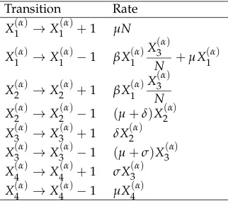
Here,µis the recruitment and per capita death rate, βis the transmission rate,δis the rate at 78

which exposed individuals become infectious, andσis the recovery rate. 79

A stochastic SEIR model can be depicted using a continuous time Markov chain (CTMC) like the 80

birth and death process with non-linear rates of transition as those given in table1, see [50, p.22] and 81

[51, p.321]. M . S . Bartlett [9] and Greenwood and Gordillo [31] introduced (integer) stochastic SIR 82

model using CTMC with rates similar to those in the first six rows in table1to show a deterministic 83

SIR model of the ODE type depicting the approximate dynamics of the means of the processes. Here, 84

we introduce a fractional SEIR model using a CTMC of fractional birth and death process on triplets 85

(i,j,k)with rates provided by table1. 86

Table 1.Transitions and their rates for a birth and death process depicting a stochastic SEIR model.

Transition Rate

X(α)

1 →X (α)

1 +1 µN

X(₁α)→X₁(α)−1 βX(₁α)X

(α) 3

N +µX

(α) 1

X(₂α)→X₂(α)+1 βX(₁α)X

(α) 3

N X(₂α)→X(₂α)−1 (µ+δ)X(₂α)

X(α)

3 →X (α)

3 +1 δX (α)

2

X(₃α)→X(₃α)−1 (µ+σ)X₃(α)

X₄(α)→X₄(α)+1 σX(₃α)

X₄(α)→X₄(α)−1 µX₄(α)

Anα-fractional SEIR stochastic process{(X₁(α)(t),X₂(α)(t),X₃(α)(t)): t≥0}for 0 < α≤1 with state probabilities

p(α)_(i,j,k)(t) =P((X₁(α)(t),X₂(α)(t),X₃(α)(t)) = (i,j,k)|(X₁(α)(0),X₂(α)(0),X₃(α)(0)) = (i0,j0,k0)

fori,j,k= 0, 1, . . ., such that 0≤ i+j+k≤ NandP((X₁(α)(0),X(α)₂ (0),X(α)₃ (0)) = (i0,j0,k0)) = 1, 87

has a fractional forward Kolmogorov equation of the stochastic SEIR model similar to equation (A1) 88

and is given by 89

Dα

∗p(α)_(i,j,k)(t) = µN p(i−(α)1,j,k)(t) +β(i+1) k Np

(α)

(i+1,j−1,k)(t) +µ(i+1)p (α) (i+1,j,k)(t)

+δ(j+1)p(α)_{(i,j+1,k−1)}(t) +µ(j+1)p_(i(α)_,j+1,k)(t) + (σ+µ)(k+1)p(α)_(i,j,k+1)(t)

−(µN+βik

N+µi+ (δ+µ)j+ (σ+µ)k)p (α)

(i,j,k)(t) (10)

with p(α)_(i,j,k)(t) = 0 if eitheri,j, orkare negative or more than N. See also Di Crescenzoet al.[45]. 90

The classical forward Kolmogorov equation of the stochastic SEIR model follows whenα=1 with 91

functionG(α)(u,v,w,t) = E(uX(1α)(t)vX

(α) 2 (t)wX

(α)

3 (t))of the state probabilities, as the solution of the 93

Cauchy problem 94

Dα

∗G(α) = µN(u−1)G(α)+µ(1−u)∂uG(α)+ (δw+µ−(δ+µ)v)∂vG(α)

+(σ+µ)(1−w)∂wG(α)+βw

N(v−u)∂uwG

(α) ₍₁₁₎

fort>0 andG(α)(u,v,w, 0) =ui0_vj0_wk0_{, for−1<u,v,w<1.} 95

Note that, the integer or classical stochastic SEIR process is(X(₁1)(t),X₂(1)(t),X₃(1)(t))which is 96

simply the case whenα =1. But that leads to another interesting fact that defines the relationship 97

between the fractional and integer stochastic SEIR model; that is, the former process is a random-time 98

subordination of the latter one, as established for other fractional processes like the fractional Poisson 99

process [37,45,52], and the fractional birth and/or death processes [39,40,42,43,53]. 100

Theorem 1. The fractional stochastic SEIR process(X(α)₁ (t),X₂(α)(t),X(α)₃ (t))has the same distribution as the random-time subordinated integer stochastic SEIR process

(X(₁1)(T2α(t)),X (1)

2 (T2α(t)),X (1)

3 (T2α(t))) for t>0and0<α≤1.

101

The proof is provided in AppendixA. 102

2.3. Measles’ Model via Fractional Differential Equations (FDE) 103

The means of the three discrete-marginal processesX₁(α)(t),X₂(α)(t), andX(α)₃ (t)can be found using∂uG(α)(1, 1, 1,t),∂vG(α)(1, 1, 1,t), and∂wG(α)(1, 1, 1,t), respectively. LetS(α)(t):= _N1E(X₁(α)(t)), E(α)(t) := _N1E(X₂(α)(t)), and I(α)(t) := _N1E(X₃(α)(t)), where N is the total population size and E(x) is the expected value of x. Thus using equation (11), and approximating E(X₁(α)(t)X(α)₃ (t)) byE(X₁(α)(t))E(X₃(α)(t))we reach the fractional order version of the system of equations that was used by M . S . Bartlett [9] to model measles,

Dα

∗S(α)=µ−βS(α)I(α)−µS(α)

Dα

∗E(α)=βS(α)I(α)−(µ+δ)E(α)

Dα

∗I(α)=δE(α)−(µ+σ)I(α)

(12)

where S(α)_{, E}(α)_{, and I}(α) _{be the proportion of susceptible, exposed, and infected individuals,} respectively. With proportion of recovered individuals given by R(α) = 1−(S(α)+E(α)+I(α)), we reach the fractionalαorder SEIR model

Dα

∗S(α)=µ−βS(α)I(α)−µS(α)

Dα

∗E(α)=βS(α)I(α)−(µ+δ)E(α)

Dα

∗I(α)=δE(α)−(µ+σ)I(α)

Dα

∗R(α)=σI(α)−µR(α)

(13)

with a powerαof new parameters; that is,θ∗αin place ofθso the parametersθ∗will have the dimension of _time1 and the system becomes the following form:

Dα

∗S(α)=µα∗−β∗αS(α)I(α)−µα∗S(α) Dα

∗E(α)=βα∗S(α)I(α)−(µα∗+δα∗)E(α) Dα

∗I(α)=δ∗αE(α)−(µα∗+σ∗α)I(α) Dα

∗R(α)=σ∗αI(α)−µα∗R(α)

(14)

2.4. Measles’ Model via Ordinary Differential Equations (ODE) 104

The following system of differential equations represents the ordinary differential equation 105

representation of the SEIR model and is the FDE model whenα=1 in equation14. 106

DS=µ−βSI−µS DE=βSI−(µ+δ)E

DI=δE−(µ+σ)I DR=σI−µR

(15)

whereµ,β,δ, andσare the model parameters described above. They all have dimensions given by 107

1

time. The last equation in (15) is redundant sinceR=1−(S+E+I). 108

2.5. Measles’ Model viaα-dependent Ordinary Differential Equations 109

We are interest in comparing the FDE vs ODE modeling approaches. It is important to note that 110

the basic ODE case considersα=1, however in the FDE case,αappears in the derivative as well as the 111

parameter values. In order to better compare these two approaches, here we develop an ODE analoge 112

to the FDE that incorporatesαin the parameter values. We call this new system theα-dependent ODE. 113

By dropping theαorder derivative from the left side andαpower fromS(α),E(α), andI(α)of equation 114

(14), ourα-dependent ODE takes the following form: 115

DS=µα∗−βα∗SI−µα∗S DE=βα∗SI−(µα∗+δ∗α)E

DI=δα∗E−(µα∗+σ∗α)I DR=σ∗αI−µα∗R

(16)

2.6. Model Analysis 116

Analysis of the ODE is almost the same as of the FDE so we include the FDE one here. We start by 117

proving the positive invariance of the region of solutions of the FDE model. Henceforth, we drop theα 118

fromS(α),E(α), andI(α), for brevity. 119

The following two lemmas of asymptotic behavior of FDEs are given here and their proof in 120

appendixAfor completeness. 121

Lemma 1. The closed simplex region M={(S,E,I)∈R3+: 0≤S+E+I≤1}is a positive invariant set 122

for the FDE model in(14). 123

We can find the model’s equilibrium points by settingDα

∗S =0,D∗αE=0, andD∗αI =0. Thus, 124

there are two equilibria to the measles’ SEIR model (14). They are: 125

2. the endemic equilibrium

EE= (s∗,e∗,i∗)≡

1 R0

, µ δ+µ

1− 1

R0

,µ

β(R0−1)

.

where the basic reproduction number isR0:= _{(µ+σ)(µ+δ)}βδ .EEexists only when 1<R0<1+β_µ. 127

An equilibrium is locally asymptotically stable if the eigenvalues of the Jacobian matrix of the 128

n-dimensional system, namelyλ1,λ2, . . . ,λn, have the property that|arg(λi)|> απ2, fori=1, 2, . . . ,n, 129

[25, p.158]. Thus, in general, the stability of the ordinary differential equations model implies stability 130

of its fractional counter model. But, here they are equivalent due to the following lemma whose 131

solution could be found in appendixA. 132

Lemma 2. The Disease-Free Equilibrium DFE is locally asymptotically stable if R0 < 1. The endemic 133

equilibrium EE is is locally asymptotically stable if R0>1. 134

Therefore, they have the same asymptotic behavior. Yet, the transient behavior differs as will be 135

seen by simulations below. 136

Moreover, a very important difference is their oscillation behavior is not similar. Letλ`andu`for

`=1, 2, . . . ,Nbe the eigenvalues and their respective eigenvectors of anN×NmatrixA. The general solution of initial value problem consisting of a system ofNlinear fractional differential equations Dα

∗x(t) =Ax(t)such thatx(0) =x0can be found to be

x(t) = N

∑

`=1

c`u`Eα(λ`tα) (17)

for certain constantsc` ∈Cfor`=1, 2, . . . ,Nsuch that∑`N=1c`u`= x0, [25, Theorem 7.13]. In case thatα=1, we recover the known solution of the system of ODEs given by

x(t) = N

∑

`=1

c`u`exp(λ`t).

IfN=3 andAis not a symmetric matrix then at least one of the eigenvalues is a real-valued number 137

and the other two eigenvalues , sayλ2andλ3, are conjugate complex-valued. In that situation,x(t) 138

would oscillate with inter-peak periods, called inter-epidemic period in disease modeling, given by 139

2π(=(λ2))−1[14]. If<(λ`) <0 for all`then the oscillations will be damped to zero. That damped 140

oscillation is clear in the case ofα=1 due to the exponential damping in the superposition of the sine 141

and cosine functions. That behavior, however, is not straight forward for 0<α<1. 142

2.7. Numerical Simulations 143

Since the mean of the subordinator process isE(T_α(t)) = t α

Γ(α+1), we use a method similar to that was introduced in Demirici and Özalp [54] to find approximate solutions to initial value FDE problems. We use that method here to simulate the solution of the FDE measles SEIR model. Consider the initial value problem

Dα

∗x(t) = f(t,x(t)), for 0<t≤T, x(0) =x0,

(18)

for someT>0. A solution of (18) is approximated by the deterministic time subordination

x(t) =y

tα

Γ(α+1)

ofy(s), the solution of the ordinary differential equation dy(s)

ds =g(s,y(s)), for 0<s≤ tα

Γ(α+1) y(0) =x0.

(20)

where

g(s,y(s)) = f(t−(tα_−sΓ( α+1))

1

α,x(t−(tα−sΓ(_α+1)) 1

α)). (21)

for all 0<t≤T, [54]. 144

We use the subordination of the solution of ODEs to FDEs represented in equations (19) and (20) 145

to numerically simulate solutions of FDEs, see algorithm1. 146

Algorithm 1Numerical solution ofDα

∗x(t) = f(t,x(t))for 0<t<Twithx(0) =x0. Input:α,T,f(t,x(t)),m,nOutput:x(t)

begin

Divide the interval[0,T]intonsub-intervals using

0=t0<t1<. . .<tn =T. fori=1, 2, . . . ,n

Divide the interval[0, t α i

Γ(α+1)]into furthermsub-intervals using

0=s0<s1<. . .<sm= tα

i

Γ(α+1).

Solve the systemDy(s) = f(ti−(tαi −sΓ(α+1)) 1

α,y(s))withy(0) =x₀using Euler or Runge-Kutta methods ons0,s1, . . . ,sm.

Retainx(ti) =y(sm). end

Return[x0,x(t1),x(t2), . . . ,x(tn)]. end

2.8. Fitting FDE and ODE models to measles data 147

We use the method of ordinary least squares (OLS) to fit the FDE model to the data by minimizing the objective function

L(α,β,µ,δ,σ) = n

∑

i=1

(I_i(d)−I_i(s))2

forα∈(0, 1], andβ,µ,δ,σ∈(0,∞), whereI(d)is the data of actual proportion of infections andI(s)is 148

the simulated proportion of infections. The valuesI_i(s)approximatingI(ti)are found by solving the 149

FDE model using algorithm1. 150

Parameter estimation was conducted using Matlab MultiStart and fmincon functions. MultiStart 151

carries out the optimization procedure using initial points within the parameters’ spaces. It generates 152

some initial points depending on a converging algorithm. The fmincon finds a local minimum for the 153

constrained nonlinear multivariable function. The MultiStart together with fimincon do the global 154

optimization of a nonlinear multivariable function. The MultiStart function uses parallel processing 155

Figure 2.Number of cases using classical ODE model and FDE model with different fractional orders

α. The simulations are done usingµ = µ? =0.0027, β = β? =119.2257,δ = δ? =16.7301, and

σ=σ? =10.1873.

0 100 200 300 400

time

1 2 3 4 5

number of cases

104

FDE with = 0.95 ODE with = 0.95 FDE with = 0.85 ODE with = 0.85

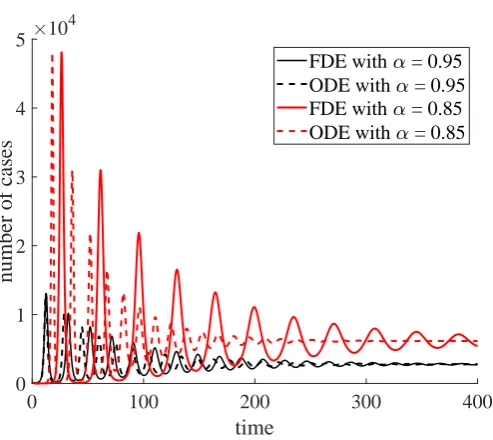
Figure 3.Number of cases using FDEM and its analogous ODEM with different fractional ordersα.

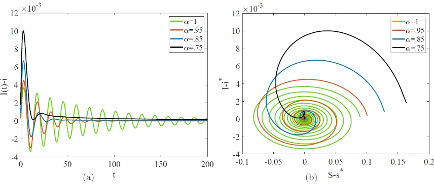
Figure 4.Simulations of solutions of the SEIR FDE centered about the endemic equilibrium (EE) for

α=1, .95, .85, and .75 using equation (17) shows a suppression of damped oscillations asαdecreases.

The simulations are done usingµ? =0.0027,β? =119.2257,δ?=16.7301, andσ?=10.1873.

3. Results 157

We solve the system of FDE (equation14) using algorithm1and the systems of ODE (equations 158

15and16) using the Runge-Kutta method. 159

Simulations of the classical ODE (equation15) and FDE ( equation14), Figure2, shows that 160

the system of fractional differential equations is very sensitive to its order of differentiationα. For 161

smallerα, the peak number of cases of the epidemic is larger but the duration of the outbreak is 162

shorter. The solution of the FDE model converges to the solution of the classical ODE asα→1. To 163

further compare the two modeling approaches, we consider the analogue ODEs derived for specificα 164

values, see equation (16). These comparisons are shown in Figure3. During transient dynamics both 165

models exhibit several peaks in the number of cases. The number of these peaks and their respective 166

amplitudes are similar between models, however there are differences in the timing of these peaks. 167

The transient oscillations of the FDE model are more stretched out than its ODE analogue, and its 168

solutions experience longer inter-epidemic times. Both models approach the same equilibria solutions. 169

Simulations of equation (17) in Figure4shows that disease models of fractional order equations 170

lack the same oscillatory behavior exhibited by systems of ODEs with conjugate complex eigenvalues 171

of the Jacobian matrices calculated at endemic equilibrium. 172

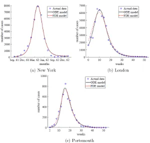
The models were fitted to three measles’ epidemics in the pre-vaccination era in three different 173

cities: New York, London, and Portsmouth. Simulations of the fitted ODE and FDE models are 174

shown in Figure5. See also AppendixBfor the data and the parameter estimates. The estimate 175

ofαare 0.99, 0.99, and 0.88 for New York, London, and Portsmouth respectively. The AIC and BIC 176

are found to be smaller for ODE models for the epidemics in New York and London with values of 177

AIC(ODE)=250.539 and 389.358 and BIC(ODE)=253.872 and 394.541, respectively, while AIC(FDE)= 178

255.360 and 413.275 and BIC(FDE)=259.526 and 419.754, respectively. For Portsmouth’s epidemic, the 179

results are the opposite, AIC(ODE)=277.938 and BIC(ODE)=282.978 while AIC(FDE)=271.920 and 180

BIC(FDE)=278.213. Yet the differences between the fitting of ODE and FDE models are not striking. 181

4. Discussion 182

Replacing first order derivatives with Caputo fractional derivatives has been the practice for 183

many studies using fractional order modeling of diseases. In this paper, we show how those models 184

follow from an approximation to the dynamical system governing the means of fractional stochastic 185

SEIR processes. Moreover, we study ordinary and fractional order systems of differential equations 186

Figure 5.Simulations of ODE and FDE models fitted to measles epidemics in the pre-vaccination era.

pre-vaccination era. It appears that, in some situations, the fractional order differential equation model 188

(FDEM) gives better fit than the ordinary differential equation model (ODEM). 189

Angstmannet al.[34] use the master equation of a continuous-time random walk to derive an 190

FDEM involving Riemann-Liouville fractional derivatives. Power laws are postulated to model time of 191

infectiousness and recovery. That extension from exponential times in ordinary differential equations 192

is a different approach from the mean field approximation of a stochastic process. Saeedianet al.[36] 193

introduced the Caputo fractional differential equations through a memory of the whole process of 194

infection and disease recovery. In our paper, we have considered, for the first time, fractional stochastic 195

SEIR model and have shown how the Caputo fractional differential equations follows as mean-field 196

approximation of the process. 197

Fractional stochastic SEIR model introduced here turns out to be a random-time subordination 198

of a classical stochastic SEIR model. Other real-life systems are modeled using a subordination of a 199

stochastic process. A subordinated process was introduced by Mandelbrot and Taylor [55] to model 200

the logarithm of market prices where the original process is a Brownian motion subordinated by a 201

stochastic time processT2α, which is the same random time process we have found here. In Mandelbrot 202

and Taylor [55], the stochastic time processT2αis called the operational time andtis the physical time. 203

Further study of the fractional stochastic SEIR model might lead to interesting dynamical 204

behaviors. For instance, it can provide more insights into the stochastic oscillations of the disease in 205

a more flexible way than their classical counterparts. Thus, studying the fractional stochastic SEIR 206

model is the next step in this work. 207

5. Conclusion 208

In this paper, we compare two deterministic models of disease: ordinary differential equations 209

(ODE) and fractional differential equations (FDE). We use three different data sets of measles epidemics 210

stochastic SEIR model. Up to our knowledge, this is the first time such a fractional stochastic process is 212

introduced and connected to the fractional order differential equations. 213

While ODE models are regularly used to model epidemics, such as measles, FDEs seem to have 214

the potential to offer improved model fitting. Rates of transition between compartments in that case 215

could be interpreted as rates with respect to an external observer with a different type of clock, may be 216

due to delay in reporting. 217

Author Contributions:Conceptualization, MR.I., A.P. and T.O.; methodology, MR.I., D.M. and T.O.; software, 218

MR.I. and T.O.; validation, MR.I. and T.O.; formal analysis, MR.I. and T.O..; investigation, MR.I. and T.O.; data 219

curation,MR.I. and T.O.; writing–original draft preparation, MR.I., D.M.,A.P. and T.O.; writing–review and editing, 220

MR.I., A.P. and T.O.; visualization, MR.I., A.P., D.M. and T.O.; supervision, A.P. and T.O.; funding acquisition, A.P. 221

Funding:A.P. was partially supported by NSF grant DMS-1815750. 222

Acknowledgments:We thanks Joshua Padgett for his valuable comments. 223

Conflicts of Interest:The authors declare that they have no competing interests. The funders had no role in the 224

design of the study; in the collection, analyses, or interpretation of data; in the writing of the manuscript, or in the 225

decision to publish the results. 226

Appendix A. Some Definitions and Proofs 227

Laplace transform of a functionf(t)is defined as

L(f)(s) = fˆ(s) =

Z ∞

0 e

−st_f(t)dt.

The inverse transform is defined by

L−1(fˆ)(t) = 1 2πi

Z

Ce

st_fˆ(s)ds

whereCis a contour parallel to the imaginary axis and to the right of the singularities of ˆf. The Laplace transform of the Caputo fractional derivative is given by

L(Dα

∗f)(s) =sαfˆ(s)−sα−1f(0). Fractional Birth and Death Process:

228

Anα-fractional nonlinear birth and death process{Nα(t) : t ≥ 0}for 0 < α ≤ 1 with state probabilities

pα

n(t) =P(Nα(t) =n|Nα(0) =1)

forn≥0 is defined through the forward Kolmogorov (difference-)differential equations Dα

∗pαn(t) =λn−1pαn−1(t) +µn+1pαn+1(t)−(λn+µn)pαn(t) (A1)

forn ≥ 0 [39,43,53]. The ratesλn andµn are non-negative. The classical birth and death process 229

follows whenα=1 with state probabilitiesp1_n(t). Whenλn=λandµn =0 for alln, theα-fractional 230

nonlinear birth and death process becomes theα-fractional Poisson process [37,41,46]. There, it has 231

shown thatNα(t)has the same probability distribution asN(Tα(t)), whereN(t)is the classical birth 232

and death process which is independent of a random time processT_α(t); that is, a birth and death 233

process subordinated by anα-stable time process. 234

The random time processTα(t)has a distribution given by the folded solution of the fractional diffusion equation∂α_tF=∂2xFfor 0<α≤2,x∈R,t>0, and subject toF(x, 0) =δ(x)for 0<α≤2 and∂α_tF(x, 0) =0 for 1<α≤2, [43]. We will denote its measure byνα,t(ds):=P(Tα(t)∈ds). It has a Laplace transform

L(να,s)(r) =

Z ∞

0 e −rt

να,t(dt) =r α 2−1_e−sr

and momentsE[(Tα(t))k] =Γ(k+1) tkα

Γ(kα+1)fork=1, 2, . . .; [46,56]. 235

Note that, the absolute values of partial derivatives ofGare finite; that is,|∂u(i,,vj,,k)wG|<∞for any 236

i,j,k=0, 1, 2, . . .. That is true since|u|,|v|,|w|<1 and the population size is finite. Thus, switching 237

integrals with derivatives or summations below are valid. 238

239

Proof of the Theorem1 240

We are going to show that Laplace transform of the probability generating function of the process

(X(₁1)(T2α(t)),X (1)

2 (T2α(t)),X (1)

3 (T2α(t)))

is the same as Laplace transform ˆGof G, that solves equation (11). From there we will conclude 241

that the two probability distributions are the same since the probability generating function of 242

(X(α)₁ (t),X(α)₂ (t),X(α)₃ (t)), by construction, is also a solution to the Cauchy problem in equation (11). 243

From equation (11), the Laplace transform ˆGis the solution of 244

sα_Gˆ(α)_−sα−1_ui0_vj0_wk0 _{= µN(u−1)G}ˆ(α)_{+µ(1−u)∂}

uGˆ(α)+ (δw+µ−(δ+µ)v)∂vGˆ(α) +(σ+µ)(1−w)∂wGˆ(α)+βw

N(v−u)∂uwGˆ

(α) _(A2)

LetH(α)(u,v,w,t)be the probability generating function of the state probabilities q_(i(α)_,j,k)(t) =P((X₁(1)(T2α(t)),X

(1)

2 (T2α(t)),X (1)

3 (T2α(t))) = (i,j,k)| (X(₁1)(T2α(0)),X

(1)

2 (T2α(0)),X (1)

3 (T2α(0))) = (i0,j0,k0)). That means that

245

H(α)(u,v,w,t) = E(uX(11)(T2α(t))_vX

(1)

2 (T2α(t))_wX

(1)

3 (T2α(t))₎

=

∑

i

∑

∑

uivjwkq(α)_(i,j,k)(t)

=

∑

i

∑

∑

Z ∞

0 p (1)

(i,j,k)(s)ν2α,t(ds) =

Z ∞

0

(

∑

∑

∑

uivjwkp(_(i1_,)_j,k)(s))ν2α,t(ds)

=

Z ∞

0 G

(1)_(u,v,w,s)

ν2α,t(ds).

Thus the Laplace transform of the probability generating functionH(α)is given by 246

ˆ

H(α)(u,v,w,r) =

Z ∞

0 e

−rtZ ∞

0 G

(1)_(u,v,w,s)

ν2α,t(ds)dt = rα−1

Z ∞

0 G

Now, the Laplace transform of the probability generating function of the process 247

(X(₁1)(t),X₂(1)(t),X₃(1)(t))also solves (A2) whenα=1 which is 248

sGˆ(1)−ui0_vj0_wk0 _{= µN(u−1)G}ˆ(1)_{+µ(1−u)∂uG}ˆ(1)_{+ (δw+µ−(δ+µ)v)∂vG}ˆ(1) +(σ+µ)(1−w)∂wGˆ(1)+βw

N(v−u)∂uwGˆ

(1)_{. (A3)}

If we substitute withs=rα_{in equation (A3) and multiply both sides byr}α−1_{we get} 249

rα_Hˆ(α)_−rα−1_ui0_vj0_wk0 _{= µN(u−1)H}ˆ(α)_{+µ(1−u)∂uH}ˆ(α)_{+ (δw+µ−(δ+µ)v)∂vH}ˆ(α) +(σ+µ)(1−w)∂wHˆ(α)+βw

N(v−u)∂uwHˆ

(α) _(A4)

which is the same as equation (A2). This completes the proof. 250

251

Proof of Lemma1 252

Starting on the S-axis whenE(0) =I(0) =0 and 1≥S(0) =S0≥0, then

S(t) =tα_E

α,α+1(−µtα)(µ) +Eα,1(−µtα)S0≥0

sinceµ>0 andt≥0. Starting on the E-axis whenS(0),I(0) =0 andE(0) =E0≥0, then

E(t) =Eα,1(−(µ+δ)tα)E0≥0 Starting on the I-axis whenS(0),E(0) =0 andI(0) =I0≥0, then

I(t) =Eα,1(−(µ+σ)tα)I0≥0 Thus, all axes are positive invariant, forS(0),E(0),I(0)≥0. 253

If the solution of the system is leaving through the positive quadrant of the E-I plane, then S(te) = 0, and E(te)and I(te) > 0 for somete > 0 such that S(t) ≤ S(te), for all t > te. But, Dα

∗S|t=te =µ>0. By the generalized mean value theorem S(t) =S(te) + _Γ1

(α)D α

∗S(τ)(t−te)α

for somete ≤τ<t, thenS(t)>S(te)contradicting the original statement. The same argument could be used for the positive quadrant of the S-I plane withDα

∗E|t=te =βS(te)I(te)>0 and for the positive quadrant of the E-S plane withDα

∗I|t=te =αE(te)>0.

To show thatS(t) +E(t) +I(t)≤1 for allt>0, ifS(0) +E(0) +I(0)≤1, Dα

∗(S+E+I) =µ−µ(S+E+I)−σI

≤µ−µ(S+E+I)

(A5)

Thus,

S(t) +E(t) +I(t)≤tα_E

α,α+1(−µtα)µ+Eα,1(−µtα)(S(0) +E(0) +I(0))

≤tα_E

α,α+1(−µtα)µ+Eα,1(−µtα) =1

(A6)

by equation (7). 254

255

For the local stability of a disease-free equilibrium, we must evaluate the Jacobian matrix at DFE≡(1, 0, 0)

J(DFE) =



 

−µ 0 −β 0 −(µ+δ) β

0 δ −(µ+σ)



 

The eigenvalues of the matrixJare,

λ1=−µ,

λ2=

−(δ+2µ+σ)−

√

∆

2 ,

λ3=

−(δ+2µ+σ) +

√

∆

2 ,

where∆=δ2+4δβ−2δσ+σ2. From this it is clear thatλ1is negative and since

∆=δ2+4δβ−2δσ+σ2= (δ−σ)2+4δβ>0

thenλ2andλ3are real-valued numbers. Henceλ2<0. But,λ3<0 is true when

−(δ+2µ+σ) +pδ2+4δβ−2δσ+σ2

2 <0

which is equivalent toβδ<(µ+σ)(µ+δ), proving the first part. 257

The Jacobian matrix calculated atEEis given by

J(EE) =



 

−µR0 0 −β_R1 0 µ(R0−1) −(µ+δ) β_R1

0

0 δ −(µ+σ)



 

which has a characteristic polynomial,

−λ3−λ2[(µ+δ) + (µ+σ) +µR0]−λ[µR0(2µ+δ+σ)] +µ(R0−1)(µ+σ)(µ+δ).

Because that polynomial has a degree of 3, we choose to test the Routh-Hurwitz conditions to see ifEEis stable.

a1=µR0+ (2µ+δ+σ)>0 a3=µ(R0−1)(µ+σ)(µ+δ)>0 With these conditions we check that the determinant,D2>0.

D2=a1a2−a3= (µR0+2µ+δ+σ)(µR0(2µ+δ+σ))−(µ(R0−1)(µ+σ)(µ+δ)) =µ[µR2₀(2µ+δ+σ) + (2µ+δ+σ)2R0−R0(µ+σ)(µ+δ) + (µ+σ)(µ+δ)] =µ[µR2₀(2µ+δ+σ) + (µ+σ)2R0+ (µ+δ)2R0+ (µ+σ)(µ+δ)R0+ (µ+σ)(µ+δ)]>0 From this, all Routh-Hurwitz conditions are met and all the eigenvalues of the Jacobian matrix at 258

Appendix B. Data Sets and Parameter Estimation 260

Appendix B.1. New York 261

Monthly reported infections of measles from September 1961 to January 1963 in New York city 262

are given in tableA1. Parameter estimation of Measles New York data from September 1961 to January 263

1963 using both ODE model and FDE model. The estimated parameters values for the classical ODE 264

model are(µ,β,δ,σ) = (0.0028, 119.22, 16.73, 10.19)with the sum of square error,SSE=1.29×106 265

and for the FDE model are(α,µ,β,δ,σ) = (0.99, 0.0029, 116.34, 19.39, 10.37)with the sum of square 266

error,SSE=1.34×106. 267

Table A1.Reported infections of measles from September 1961 to January 1963 in New York, US.

Year Months Cases Year Months Cases Year Months Cases 1961 September 109 1962 March 5839 1962 September 58 1961 October 123 1962 April 7875 1962 October 86 1961 November 383 1962 May 6555 1962 November 125 1961 December 1043 1962 June 2866 1962 December 145 1962 January 1725 1962 July 1075 1963 January 184 1962 February 3056 1962 August 266

Appendix B.2. London 268

Biweekly reported infections of measles in 1961 in London, United Kingdom are given in table 269

A2. Parameter estimation of measles Portsmouth data in 1961 using both ODE model and FDE 270

model. The estimated parameters values for the classical ODE model are (µ,β,δ,σ) = (6.79× 271

10−4, 153.44, 1.99, 4.27)with the sum of square error, SSE= 2.01×106and for the FDE model are 272

(α,µ,β,δ,σ) = (0.99, 8.53×10−4, 62.89, 5.37, 4.95)with the sum of square error,SSE=4.37×106. 273

Table A2.Biweekly reported measles infections in 1961 in London, UK.

Year Weeks Cases Year Weeks Cases Year Weeks Cases Year Weeks Cases

1961 0 1636 1961 14 5374 1961 28 514 1961 42 89

1961 2 2700 1961 16 4272 1961 30 375 1961 44 87

1961 4 2639 1961 18 2322 1961 32 265 1961 46 73

1961 6 4805 1961 20 1810 1961 34 199 1961 48 70

1961 8 6543 1961 22 1409 1961 36 121 1961 50 59

1961 10 6389 1961 24 1037 1961 38 86 1961 52 45

1961 12 5545 1961 26 767 1961 40 76

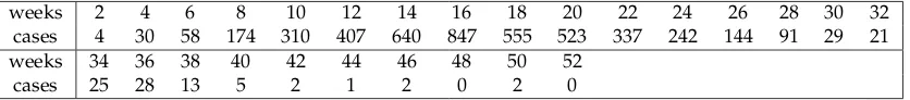
Appendix B.3. Portsmouth 274

Biweekly reported infections of measles in 1961 in Portsmouth, United Kingdom are given in table 275

A3. Parameter estimation of measles Portsmouth data in 1961 using both ODE model and FDE model. 276

The estimated parameters values for the classical ODE model are(µ,β,δ,σ) = (10−6, 228.61, 0.46, 3.33) 277

with the sum of square error,SSE=4.57×104and for the FDE model are(α,µ,β,δ,σ) = (0.88, 2.56× 278

10−4, 278.72, 1.52, 5.24)with the sum of square error,SSE=3.22×104. 279

Table A3.Biweekly reported infections of measles in 1961 in Portsmouth, UK.

weeks 2 4 6 8 10 12 14 16 18 20 22 24 26 28 30 32

cases 4 30 58 174 310 407 640 847 555 523 337 242 144 91 29 21

weeks 34 36 38 40 42 44 46 48 50 52

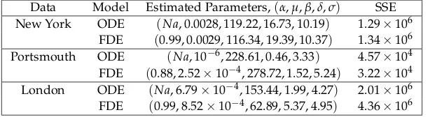
Appendix B.4. Parameter Estimations 280

Table A4.Comparison between the classical ODE model and FDE model using different data sets

Data Model Estimated Parameters,(α,µ,β,δ,σ) SSE

New York ODE (Na, 0.0028, 119.22, 16.73, 10.19) 1.29×106 FDE (0.99, 0.0029, 116.34, 19.39, 10.37) 1.34×106 Portsmouth ODE (Na, 10−6, 228.61, 0.46, 3.33) 4.57×104 FDE (0.88, 2.52×10−4, 278.72, 1.52, 5.24) 3.22×104 London ODE (Na, 6.79×10−4, 153.44, 1.99, 4.27) 2.01×106 FDE (0.99, 8.52×10−4, 62.89, 5.37, 4.95) 4.36×106

281

References 282

1. Bernoulli, D. Essai d’une nouvelle analyse de la mortalité causée par la petite vérole. InMém Math Phys

283

Acad Roy Sci Paris; 1766; Vol. 1, pp. 1–45. 284

2. Ross, R. An Application of the Theory of Probabilities to the Study of a priori Pathometry. Part 285

I. Proceedings of the Royal Society A: Mathematical, Physical and Engineering Sciences1916, 92, 204–230. 286

doi:10.1098/rspa.1916.0007. 287

3. Brownlee, J. Certain Aspects of the Theory of Epidemiology in Special Relation to Plague.Proceedings of

288

the Royal Society of Medicine1918,11, 85–132. 289

4. Greenwood, M.; Yule, G.U. An Inquiry into the Nature of Frequency Distributions Representative of 290

Multiple Happenings with Particular Reference to the Occurrence of Multiple Attacks of Disease or of 291

Repeated Accidents. Journal of the Royal Statistical Society1920,83, 255. doi:10.2307/2341080. 292

5. Kermack, W.O.; McKendrick, A.G. A Contribution to the Mathematical Theory of Epidemics.Proceedings

293

of the Royal Society A: Mathematical, Physical and Engineering Sciences1927. doi:10.1098/rspa.1927.0118. 294

6. Soper, H.E. The Interpretation of Periodicity in Disease Prevalence. Journal of the Royal Statistical Society

295

1929,92, 34. doi:10.2307/2341437. 296

7. Greenwood, M. On the Statistical Measure of Infectiousness.The Journal of hygiene1931,31, 336–51. 297

8. Greenwood, M. The statistical study of infectious diseases. Journal of the Royal Statistical Society. Series A

298

(General)1946,109, 85–110. 299

9. M . S . Bartlett. Some Evolutionary Stochastic Processes. Journal of the Royal Statistical Society . Series B (

300

Methodological )1949,11, 211–229. 301

10. Bailey, N.T.J. The Total Size of a General Stochastic Epidemic.Biometrika1953,40, 177. doi:10.2307/2333107. 302

11. Bailey, N.T.J.The mathematical theory of infectious diseases and its applications; Griffin, 1975; p. 413. 303

12. Anderson, R.M.The Population dynamics of infectious diseases : theory and applications; 1982. 304

13. Hethcote, H.W. The Mathematics of Infectious Diseases. SIAM Review 2005. 305

doi:10.1137/s0036144500371907. 306

14. Keeling, M.J.; Danon, L. Mathematical modelling of infectious diseases, 2009. doi:10.1093/bmb/ldp038. 307

15. Anderson, R.M.; May, R.M. Infectious Diseases of Humans: Dynamics and Control (Oxford Univ. Press,

308

Oxford1991. 309

16. Castillo-Chavez, C.; Blower, S.; van den Driessche, P.; Kirschner, D.; Abdul-Aziz, Y.Mathematical Approaches

310

for Emerging an Reemerging Infectious Diseases; 2002. doi:10.1007/978-1-4613-0065-6. 311

17. Temime, L.; Hejblum, G.; Setbon, M.; Valleron, A. The rising impact of mathematical modelling in 312

epidemiology: antibiotic resistance research as a case study. Epidemiology and Infection2008,136, 289. 313

doi:10.1017/S0950268807009442. 314

18. Fisman, D.N.; Hauck, T.S.; Tuite, A.R.; Greer, A.L. An IDEA for Short Term Outbreak 315

Projection: Nearcasting Using the Basic Reproduction Number. PLoS ONE 2013, 8, e83622. 316

doi:10.1371/journal.pone.0083622. 317

19. Ahmed, E.; Elgazzar, A.S. On fractional order differential equations model for nonlocal epidemics. Physica

318

20. Demirci, E.; Unal, A.; Özalp, N. A fractional order SEIR model with density dependent death rate.Hacettepe

320

Journal of Mathematics and Statistics2011. 321

21. Al-Sheikh, S.A. Modeling and Analysis of an SEIR Epidemic Model with a Limited Resource for Treatment 322

Modeling and Analysis of an SEIR Epidemic Model with a Limited Resource for Treatment Modeling 323

and Analysis of an SEIR Epidemic Model with a Limited Resource for Treatme. Type : Double Blind Peer

324

Reviewed International Research Journal Publisher: Global Journals Inc2012,12. 325

22. Diethelm, K. A fractional calculus based model for the simulation of an outbreak of dengue fever.Nonlinear

326

Dynamics2013. doi:10.1007/s11071-012-0475-2. 327

23. Li, J.; Cui, N. Dynamic analysis of an SEIR model with distinct incidence for exposed and infectives. The

328

Scientific World Journal2013,2013, 1–5. doi:10.1155/2013/871393. 329

24. El-Shahed, M.; El-Naby, F.A. Fractional calculus model for for childhood diseases and vaccines. Applied

330

Mathematical Sciences2014,8, 4859–4866. doi:10.12988/ams.2014.4294. 331

25. Dold, E.A.; Eckmann, B.; Accola, R.D.M.Lecture Notes in Mathematics Springer-Verlag; 1975. 332

26. Almeida, R.; Brito da Cruz, A.M.; Martins, N.; Monteiro, M.T.T. An epidemiological MSEIR model 333

described by the Caputo fractional derivative. International Journal of Dynamics and Control2018, pp. 1–14. 334

doi:10.1007/s40435-018-0492-1. 335

27. Area, I.; Batarfi, H.; Losada, J.; Nieto, J.J.; Shammakh, W.; Torres, Á. On a fractional order Ebola epidemic 336

model. Advances in Difference Equations2015. doi:10.1186/s13662-015-0613-5. 337

28. Haggett, P.The geographical structure of epidemics; Clarendon Press, 2000; p. 149. 338

29. Bjørnstad, O.N.; Finkenstädt, B.F.; Grenfell, B.T. Dynamics of Measles Epidemics : Estimating Scaling of. 339

Ecological Monographs2002,72, 169–184. 340

30. Yingcun Xia.; Ottar N. Bjørnstad.; Bryan T. Grenfell. Measles Metapopulation Dynamics: A Gravity Model 341

for Epidemiological Coupling and Dynamics. The American Naturalist2004. doi:10.1086/422341. 342

31. Greenwood, P.E.; Gordillo, L.F. Stochastic epidemic modeling. InMathematical and Statistical Estimation

343

Approaches in Epidemiology; 2009; pp. 31–52. doi:10.1007/978-90-481-2313-1_2. 344

32. Vasilyeva, O.; Oraby, T.; Lutscher, F. Aggregation and environmental transmission in Chronic Wasting 345

Disease.Mathematical Biosciences and Engineering2015,12. doi:10.3934/mbe.2015.12.209. 346

33. Aranda, D.F.; Trejos, D.Y.; Valverde, J.C. A fractional-order epidemic model for bovine Babesiosis disease 347

and tick populations. Open Physics2017,15, 360–369. doi:10.1515/phys-2017-0040. 348

34. Angstmann, C.; Henry, B.; McGann, A. A Fractional-Order Infectivity and Recovery SIR Model. Fractal and

349

Fractional2017,1, 11. doi:10.3390/fractalfract1010011. 350

35. Sardar, T.; Rana, S.; Chattopadhyay, J. A mathematical model of dengue transmission with 351

memory. Communications in Nonlinear Science and Numerical Simulation 2015, 22, 511–525. 352

doi:10.1016/j.cnsns.2014.08.009. 353

36. Saeedian, M.; Khalighi, M.; Azimi-Tafreshi, N.; Jafari, G.R.; Ausloos, M. Memory effects on epidemic 354

evolution: The susceptible-infected-recovered epidemic model. Physical Review E2017, [1703.03191]. 355

doi:10.1103/PhysRevE.95.022409. 356

37. Laskin, N. Fractional Poisson process2003. 8, 201–213. doi:10.1016/S1007-5704(03)00037-6. 357

38. UCHAIKIN, V.V.; CAHOY, D.O.; SIBATOV, R.T. FRACTIONAL PROCESSES: FROM POISSON 358

TO BRANCHING ONE. International Journal of Bifurcation and Chaos 2008, 18, 2717–2725. 359

doi:10.1142/s0218127408021932. 360

39. Orsingher, E.; Polito, F.; Sakhno, L. Fractional Non-Linear, Linear and Sublinear Death Processes. Journal of

361

Statistical Physics2010,141, 68–93. doi:10.1007/s10955-010-0045-2. 362

40. Orsingher, E.; Polito, F. Fractional pure birth processes. Bernoulli2010,16, 858–881. doi:10.3150/09-bej235. 363

41. Meerschaert, M.M.; Nane, E.; Vellaisamy, P. The fractional poisson process and the inverse stable 364

subordinator.Electronic Journal of Probability2011,16, 1600–1620. doi:10.1214/EJP.v16-920. 365

42. Garra, R.; Polito, F. A note on fractional linear pure birth and pure death processes in epidemic models. 366

Physica A: Statistical Mechanics and its Applications2011,390, 3704–3709. doi:10.1016/j.physa.2011.06.005. 367

43. Orsingher, E.; Polito, F. On a fractional linear birth–death process. Bernoulli 2011, 17, 114–137. 368

doi:10.3150/10-bej263. 369

44. Orsingher, E.; Ricciuti, C.; Toaldo, B. Population models at stochastic times. Advances in Applied Probability

370

45. Di Crescenzo, A.; Martinucci, B.; Meoli, A. A fractional counting process and its connection with the 372

poisson process.Alea2016,13, 291–307. 373

46. Kumar, A.; Leonenko, N.; Pichler, A. Fractional Risk Process in Insurance2018. pp. 1–25,[1808.07950]. 374

47. Podlubny, I. Geometric and Physical Interpretation of Fractional Integration and Fractional Di ff erentiation 375

2008. pp. 1–18,[arXiv:arXiv:math/0110241v1]. 376

48. Özalp, N.; Demirci, E. A fractional order SEIR model with vertical transmission 2011. 54, 1–6. 377

doi:10.1016/j.mcm.2010.12.051. 378

49. Earn, D.J.; Rohani, P.; Bolker, B.M.; Grenfell, B.T. A simple model for complex dynamical transitions in 379

epidemics. Science2000. doi:10.1126/science.287.5453.667. 380

50. Allen, L.J.S.Stochastic Population and Epidemic Models; 2015. doi:10.1007/978-3-319-21554-9. 381

51. Allen, L. An Introduction to Stochastic Processes with Applications to Biology, Second Edition; 2018. 382

doi:10.1201/b12537. 383

52. Di Crescenzo, A.; Meoli, A. On a fractional alternating Poisson process. AIMS Mathematics, pp. 212–224. 384

doi:10.3934/math.2016.3.212. 385

53. Konno, H.; Pázsit, I. Fractional Linear Birth-Death Stochastic Process—An Application of Heun’s 386

Differential Equation.Reports on Mathematical Physics2018,82, 1–20. doi:10.1016/S0034-4877(18)30062-4. 387

54. Demirici, E.; Özalp, N. A method for solving differential equations of fractional order. Journal of

388

Computational and Applied Mathematics2012,236, 2754–2762. doi:10.1016/j.amc.2015.05.049. 389

55. Mandelbrot, B.; Taylor, H.M. On the Distribution of Stock Price Differences. Operations Research1967, 390

15, 1057–1062. doi:10.1287/opre.15.6.1057. 391

56. Piryatinska, A.; Saichev, A.; Woyczynski, W. Models of anomalous diffusion: the subdiffusive case. Physica

392