A two-dimensional generalized initially
stressed magneto-thermoelastic problem for
a half-space with voids
SUNITA DESWAL and NEELAM HOODA*
Department of Mathematics
Guru Jambheshwar University of Science and Technology Hisar-125001,Haryana,India.
Email addresses:[email protected](S.Deswal), [email protected](Neelam).
Abstract
The present work is aimed at the analysis of the response of a homogeneous, isotropic, generalized thermoelastic half-space with voids permeated into a uniform magnetic field parallel to the bounding plane due to mechanical load acting on the initially stressed surface. The problem is studied in the context of generalized thermoelasticity with one relaxation time. Normal mode analysis is used to obtain the expressions for displacements, stresses, temperature distribution and change in volume fraction field for thermally insulated as well as isothermal boundaries. Comparisons are made with the results predicted in the presence and absence of voids and initial stress.
Keywords: Generalized thermoelasticity; Magnetic field; Voids; Hydrostatic initial stress; Normal mode analysis.
1. Introduction
The heat conduction equations for the classical linear uncoupled and coupled thermoelasticity theories are of the diffusion type predicting infinite speed of propagation for heat wave contrary to physical observations. To eliminate this paradox inherent in the classical theories, non-classical theories (generalized theories) of thermoelasticity were developed. The generalized thermoelasticity theories admit so-called second-sound effects, that is, they predict finite velocity of propagation for heat field. The first attempt towards the introduction of generalized thermoelasticity was headed by Lord and Shulman [1], who formulated the theory by incorporating a flux-rate term into conventional Fourier’s law of heat conduction. The L-S (Lord-Shulman) theory introduces a new constant that acts as a relaxation time. Since the heat conduction equation of this theory is of the wave-type, it automatically ensures finite speed of propagation for heat wave. The second generalization was developed by Green and Lindsay [2]. This theory contains two constants that act as relaxation times and modifies all the equations of coupled theory, not the heat conduction equation only.
Theory of elastic materials with voids is one of the most important generalizations of the classical theory of elasticity. This theory is concerned with elastic materials consisting of a distribution of small pores (voids, which contain nothing of mechanical or energetic significance) in which the void volume is included among the kinematic variables. Practically this theory is useful for investigating various types of geological and biological materials for which elastic theory is inadequate.
diffusion material with voids with the help of L-S theory to show the existence of four coupled longitudinal waves and a shear wave.
The study of dynamic response of an isotropic generalized thermoelastic solid with additional parameters is helpful in solving many practical problems. Initial stresses are developed in the medium due to many reasons, resulting from difference of temperature, process of quenching, gravity variations, etc. The earth is supposed to be under high initial stresses. It is therefore of great interest to study the effect of these stresses on the mechanical and thermal state of the medium. Montanaro [13] investigated isotropic linear thermoelasticity with hydrostatic initial stress. Ailawalia and Singh [14] studied the effect of rotation in a generalized thermoelastic medium with hydrostatic initial stress subjected to ramp-type heating and loading. Singh et al.
[15] and Singh [16] discussed the reflection of thermoelastic waves from a free surface under hydrostatic initial stress in the context of different theories of generalized thermoelasticity.
Investigation of the interaction between magnetic field and stress and strain in a thermoelastic solid is very important due to its many applications in the fields of geophysics, plasma physics and related topics. Especially in nuclear fields, the extremely high temperature and temperature gradients, as well as the magnetic fields originating inside nuclear reactors influence their design and operations. Sherief and Helmy [17] dealt with a two-dimensional problem for a half-space in magneto thermoelasticity with thermal relaxation. Youssef [18] has examined the generalized magneto thermoelasticity in a conducting medium with variable material properties. Nayfeh and Nemat-Nasser [19] studied the propagation of plane waves in a thermoelastic solid with electric and magnetic permeability.
The present investigation is aimed at the study of the general plane strain problem of generalized electro-magneto-thermoelastic initially stressed half-space with voids due to applied mechanical load. Normal mode analysis technique is used for finding the expressions for the variables considered. Both isothermal as well as insulated boundaries are considered. Our investigation is very useful in the field of geomechanics as it models a practically possible half-space due to presence of magnetic field, initial stress, void parameters and externally applied mechanical load.
Nomenclature
ij
t
components of stress tensor,
Lame’s counterparts
3
2
tt
coefficient of linear thermal expansionT absolute temperature
0
T
reference temperaturei
u
components of displacement vector
density of the mediumij
e
components of strain tensork k
e
e, cubical dialatationk
thermal conductivity0
thermal relaxation timee
c
specific heat at constant strain
change in volume fraction field
ij Kronecker deltap
pressure1
,
b
,
,
m
,
material constants due to presence of voids0
magnetic permeability0
electric permittivityt
time variableE
Young’s modulus
initial stress parameter
gradient operator2
Laplacian operator2. Formulation of the problem and basic equations
We consider a homogeneous, isotropic, thermally conducting elastic half space
z
0
with voids under hydrostatic initial stress. z-axis is pointing vertically into the medium. The surface (z = 0) of the half space is subjected to a mechanical load. All the considered functions are assumed to be bounded and vanish as
z
. The whole body is at a uniform temperature T0. A magnetic fieldH
0,
H
0, 0
is acting towards
positive direction of y-axis. Due to application of this magnetic field, there results an induced magnetic field
h
and an induced electric field
E
. We assume that bothh
andE
are small in magnitude in accordance with the assumptions of the linear theory of thermoelasticity. All the quantities considered will be functions of the time variable t and of coordinates x and z. The components of displacement vectoru
have the following form
, ,
,
0,
, ,
u
u x z t
v
w
w x z t
.Initial magnetic field vector
H
is given by0
0, , 0
x y z
H H H H .
The electric field intensity vector is normal to both the magnetic intensity and the displacement vector. Therefore,
E
has the components1
,
0,
3
x y z
E
E
E
E
E
.The current density vector
J
, parallel toE
, has the components
1
,
0,
3
x y z
J
J
J
J
J
.The simplified linear equations of electrodynamics for a slowly moving perfectly conducting medium are
0
E
curl h
J
t
, (1)0
h
curl E
t
, (2)
0
u
E
H
t
, (3)
0
div h
. (4)
From above equations, we can obtain
1
0 0,
3
0 0
w
u
E
H
E
H
t
t
, (5)1
0,
2
0,
3
0
h
h
H e h
, (6)2 2
1
0 0 0 2,
3
0 0 0 2
w
u
J
H
J
H
t
t
. (7)Strain-displacement relation is
, ,
1
2
ij i j j i
e
u
u
. (8)Equation (8) in our case gives
1
,
,
2
xx zz xz
u
w
u
w
e
e
e
x
z
z
x
0
xy yy yz
The cubical dialatation e is given by
xx yy zz
u
w
e
e
e
e
x
z
. (9)Following Lord-Shulman [1], Iesan [10] and Montanaro [13], the field equations in terms of the displacement, volume fraction field and temperature for a linear homogeneous, isotropic initially stressed, generalized magneto-thermoelastic solid with voids in the absence of heat sources and extrinsic equilibrated body forces are
2
(
)
(
0)
,
2
2
p
p
u
u
T T
b
F
u
(10)
2 1 0b
u
m T
T
, (11)
,ii 0 kk 0 kk 0
(
0)
e 0kT
T e
e
mT
c T
T
, (12)and
t
ij
iju
k k,
u
i j,
u
j i,
b
ij
T
T
0
ij
p
ij
ij
, (13)where
, ,
1
2
ij
u
j iu
i j
andF
is the Lorentz force given by
0
F
J
H
. (14)From Eqs. (7) and (14), we obtain
2 2
2 2 2 2
0 0 0 2
,
0,
0 0 0 2x y z
u
w
F
H
F
F
H
t
t
. (15) For x-z plane, Eq. (10) gives rise to following two equations2 2
2 2 2
0 0 0
2 2
2
2
u
p
e
p
T
u
u
b
H
t
x
x
x
t
, (16)2 2
2 2 2
0 0 0
2 2
.
2
2
w
p
e
p
T
w
w
b
H
t
z
z
z
t
(17)To facilitate the solution, the following non-dimension quantities are introduced
* * * *
*
1 1 1 1
1
2 2 2 2
,
,
,
,
x
z
z t
t u
u w
w
c
c
c
c
,
2 *0 1 *
0 1 0
2 2
,
,
2
T
T
T
c
, 0 0 0,
,
,
zx zz
zx zz
t
t
p
t
t
p
T
T
T
(18)where 2
2
c
and2 2 1 e
c c
k
.Making use of Eq. (18) into Eqs. (16), (17), (11) and (12) respectively; we obtain (after suppressing primes)
2
2 2 2 2
1 2
1
1
u
e
T
u
a
t
x
x
x
, (19)
2
2 2 2 2
1 2
1
1
w
e
T
w
a
t
z
z
z
, (20)
2
2 3 4 5
a
u
a
a T
a
, (21)2
1
1
0 61
0
T
e a
T
where
2 2
2 2 0 0 2
1 2
0 0 0
2
1
,
1
,
,
2
A AH
c
c
c
T p
c
,
2 2 2 2 0 2 2 1 1* 0 1
1
,
2
2
T c
bc
a
T p
k
, 2 2 21 2 2
2 3 * 4 5
1
(
2 )
,
c
,
,
c
b
m
a
a
a
a
and
3 4 0 2 6 * 12
mT c
a
k
.The expressions relating displacement components
u x z t
, ,
and
w x z t
, ,
to the potentials
1
, ,
and
2, ,
x z t
x z t
in dimensionless form are1 2 1 2
,
u
w
x
z
z
x
. (23)Inserting Eq. (23) into Eqs. (19)-(22), we obtain
2
2 1 2 2 2
1 2 1 1
0
t
T
a
, (24)2
2 2 2 1 2 2
0
t
, (25)2 2
2 1 3 4 5
a
a
a T
a
, (26)2 2
1
1
0 1 61
0
T
a
T
t
t
t
t
t
. (27)3. Normal mode analysis
The solution of the considered physical variables can be decomposed in terms of normal modes in the following form
* * * * * * *
1 2 1 2
, ,
,
, , ,
ij, ,
,
,
,
, ,
ij,
exp
u w
t T
x z t
u w
t T
z
t
ax
(28)where ω is the complex time constant,
1
, a is the wave number in the x-direction and starred quantities are the amplitudes of the field quantities. Eqs. (24)-(27) with the aid of Eq. (28) become respectively
2 2 * * 2 *
7 1 1
0
D
a
z
a
z
T
z
, (29)
2 2
*
1
20
D
k
z
, (30)
2 2
*
2
*
*
2
1
8
4
0
a
D
a
z
D
a
z
a T
z
, (31)
2
*
*
2
*
11 12
1 13
100
a D
a
z
a
z
D
a
T
z
, (32)where
D
,
a
7a
2 1 2,
k
12a
2 2 1 2,
a
8a
2a
3 2a
5z
,
2 29
1
0,
10 9,
11 1 9,
12 11,
13 6 9.
a
a
a
a
a
a
a
a a
a
a a
Eliminating
T
*
z
and
*
z
among Eqs. (29), (31) and (32), we obtain the following sixth order partial differential equation satisfied by
1*
z
6 4 2
*
1 2 3 1
0
D
d D
d D
d
z
(33)where
d
1f
12,
d
2f
22,
d
3f
32
,f
1
2a
11
g
4
a
10
2,2 2
2 11 1 12 13 2 6 10 4
2
3
1 12
13
3
10 5f
g a
a
g
a g
,and
g
1
a a
1 4
2a
8,
g
2
a
2
a
4,
g
3
a a
4 7
a a
2 2,
2 2 4 1 2 7 8
g
a a
a
a
,g
5
a a
7 8
2
a a a
2 1 2.In a similar manner, we can show that
T
*
z
and
*
z
satisfy the equations
6 4 2
*
1 2 3
0
D
d D
d D
d T
z
, (34)
6 4 2
*
1 2 3
0
D
d D
d D
d
z
. (35)The auxilliary equation of the above differential equations given by (33), (34) and (35) is
6 4 2
1 2 3
0
D
d D
d D
d
. This equation can be factorized as
2 2
2 2
2 2
2 3 4
0
D
k
D
k
D
k
,where
k
22,
k
32and
k
42 are the roots of the characteristic equation6 4 2
1 2 3
0
k
d k
d k
d
, and are given by
2 1 3 1
1
1
2 sin
,
sin
3 cos
3
3
k
p
q d
k
d
p
q
q
,
4 1
1
sin
3 cos
3
k
d
p
q
q
,
1 2 1 2
sin
3
,
3
r
p
d
d
q
,
2
3/ 21
3
2 32
A
r
d
d
p
andA
9
d d
1 2
2
d
13
27
d
3. The solution of Eq. (30) which is bounded asz
is given by
1*
2 1
( , )
k z
z
R a
e
, (36)
where
R a
1
,
is a parameter depending on a and
. Similarly, the solutions of Eqs. (33), (34) and (35) can be written as:
4* 1
2
( , )
k zii i
z
R a
e
, (37)
4
*
2
,
k zii i i
z
a R a
e
, (38)
4
*
2
,
k zii i i
T
z
b R a
e
. (39)where
2 2 2 3 * 2 2 1 i i i
g k
g
a
k
g
and2 4 2 4 5 2 2 1 i i i i
k
g k
g
b
k
g
(i
2, 3, 4
). (40)From Eq. (23), we get
* * *
1 2
u
z
a
z
D
z
, (41)
* * *
1 2
w z
D
z
a
z
. (42)Inserting Eqs. (36) and (37) into Eqs. (41) and (42), the displacement components u and w, which are bounded as
z
are obtained as
14
1 1 2
,
k zj,
k z t axj j
u
a
R a
e
k R a
e
e
, (43)
14
1 2
,
k zj,
k z t axj j j
w
k R a
e
aR a
e
e
Stress components are of the form
14
2 2 2 2
2 1 2 1 1
2
2
,
,
2
j
k z k z t ax
zx j j
j
p
t
a
k R a
e
k
a
k
a
R a
e
e
, (45)
14
2 2 * 2 *
1 2 1 1 2 1
2
2
,
k zj2
( , )
k z t axzz j j j j
j
t
k
a
b
a
b a
R a
e
ak
R a
e
e
p
, (46)where 1 2
0 0
2
,
T
T
and 22 2 1 *
0 1
bc
b
T
.4. Application Mechanical load on the surface of the half space
4.1. Case I: Isothermal boundary
The surface z = 0 is taken to be isothermal. Hence the boundary conditions in this case are
0
,
zz zz
t
p
p
x t
,t
zx
0
,T
0
,
0,
at 0
z
z
(47)where
p
0
x t
,
is a given function x and t and
zj
j
x y z
, ,
is the Maxwell stress given in the form
0
,
, ,
zj
H h
z jH h
j zH h
k k zjj
x y z
. (48)Using Eqs. (38)-(39) and Eqs. (45)-(46) into the boundary conditions along with 0 0
0
p
p
T
; we obtain the boundary conditions in the dimensionless form. On suppressing the primes and invoking normal mode analysis (Eq. (28) ), we obtain the following system of equations1 1
2 2
3 3
4 4
0
L R
L R
L R
L R
,1 1 2 2 3 3 4 4 0
M R
M R
M R
M R
p
,2 2
3 3
4 4
0
V R
V R
V R
,2 2
3 3
4 4
0
Q R
Q R
Q R
. (49)where 1
12 2
12 2
2,
12
1 2,
2
22
j jp
L
k
a
k
a
M
ak
L
a k
,
2 2 *
2 *
2 2
1
2
2 1 3j j j j j
M
k
a
b
a
b a
k
a
,V
j
b
*j and
Q
j
a k
*j j,
j
2,3, 4
.Solution of the system of Eqs. (49) can be written as
3
1 2 4
1
,
2,
3,
4
R
R
R
R
. (50)where
L M
1 2
L M
2 1
V Q
3 4
V Q
4 3
L M
1 3
L M
3 1
Q V
2 4
Q V
4 2
L M
1 4
L M
4 1
V Q
2 3
V Q
3 2
,
1
p
0L V Q
2 3 4V Q
4 3L V Q
3 4 2V Q
2 4L V Q
4 2 3V Q
3 2
,
2
p L V Q
0 1 4 3V Q
3 4
,
3p L V Q
0 1
2 4
V Q
4 2
and
4p L V Q
0 1
3 2
V Q
2 3
. Displacement components, stress components, temperature field and change in volume fraction field are given by1
4 1 1
2
1
k z k zj t axj j
u
k
e
a
e
e
1
4 2
1
k z k zj t axj j j
w
ae
k
e
e
, (52)
14 2 2 2 2
1 1 2 1 2
2
1
2
2
j
k z
k z t ax
zx j j
j
p
t
k
a
k
a
e
a
k
e
e
, (53)
1
4
2 2 * 2 *
1 2 1 1 2 1
2
1
2
k z2
k zj t axzz j j j j
j
t
ak
e
k
a
b
a
b a
e
e
p
, (54)4 * 2
1
k zj t axj j j
T
b
e
e
, (55)4 * 2
1
k zj t axj j j
a
e
e
. (56)4.2. Case II: Insulated boundary
The surface z = 0 is taken to be insulated. Hence the boundary conditions in this case are
0
,
zz zz
t
p
p
x t
,t
zx
0
,
0
T
z
,0,
at
0
z
z
(57)where
p
0
x t
,
is a given function of x and t.Using the required expressions of the variables into the boundary conditions along with 0 0
0
p
p
T
andapplying normal mode analysis, we obtain the following system of equations
1 1
2 2
3 3
4 4
0
L R
L R
L R
L R
,1 1 2 2 3 3 4 4 0
,
M R
M R
M R
M R
p
2 2 2
3 3 3
4 4 4
0
k V R
k V R
k V R
,2 2
3 3
4 4
0
Q R
Q R
Q R
. (58)The corresponding expressions for the components of displacement, stress, temperature distribution and change in volume fraction field are given by Eqs. (51)-(56) with
replaced by
* and
js
replaced by
'
*
1, 2, 3, 4
j
s
j
*
1 2 2 1 3 3 4 4 4 3 1 3 3 1 4 4 2 2 2 4
L M
L M
k V Q
k V Q
L M
L M
k V Q
k V Q
L M
1 4
L M
4 1
k V Q
2 2 3
k V Q
3 3 2
,
*
1
p
0L k V Q
2 3 3 4k V Q
4 4 3L k V Q
3 4 4 2k V Q
2 2 4L k V Q
4 2 2 3k V Q
3 3 2
,
*
2
p L k V Q
0 1 4 4 3k V Q
3 3 4
,
*3p L k V Q
0 1
2 2 4
k V Q
4 4 2
,
*
4
p L k V Q
0 1 3 3 2k V Q
2 2 3
.5. Special cases
5.1. Neglecting the void effect
(a) Neglecting the material constants due to the presence of voids i.e.
b
1m
0 ;
we obtain the expressions for the displacement components, stresses and temperature field in the generalized initially stressed magneto-thermoelastic medium due to the mechanical load applied on the isothermal boundary1 6 ** ** 1 1 ** 5
1
k z k zj t axj j
u
k
e
a
e
e
, (59)1 6 ** ** 1 ** 5
1
k z k zj t axj j j
w
a
e
k
e
e
, (60)
16
2 2 2 2 ** **
1 1 2 1 2
** 5
1
2
2
j k zk z t ax
zx j j
j
p
t
k
a
k
a
e
a
k
e
e
, (61)
1
6
** 2 2 * 2 **
1 2 1 1 2
**
5
1
2
k z2
k zj t axzz j j j
j
t
ak
e
k
a
c
a
e
e
p
, (62)6 * ** **
5
1
k zj t axj j j
T
C
e
e
, (63)where
k
52,
k
62 are roots of the equation4 2
1 2
0
k
l k
l
. (64)with
l
1
a
7
a
10
a
11,
l
2
a a
7 10
a
12 , (65)and
**L
**1
M W
5** 6
M W
6** 5
M
1**
L W
**6 5
L W
**5 6
,** ** ** 1
p
0
L W
5 6L W
6 5
,
**5p L W
0 1** 6 ,
**6p L W
0 **1 5,
** 2 2 2 2
1 5 5 2
2
p
L
k
a
k
a
,M
1**
2
ak
5 2,**
2
2
j j
L
a k
,M
**j
k
2j
a
2
C
*j
1
2
a
2
2
k
2j
a
2
3,* 2 7
,
j j
C
k
a
W
j
C
*j,
j
5, 6
.(b) Neglecting void parameters, the expressions for the field variables due to mechanical load applied on the insulated boundary are given by Eqs. (59)-(63) with
** replaced by
*** and
**j ’s replaced by***
j ’swhere
***L
**1
M Y
5** 6
M Y
6** 5
M
1**
L Y
**6 5
L Y
**5 6
,
*** ** ** 1
p
0L Y
5 6L Y
6 5
,
***5p L Y
0 **1 6,
***6p L Y
0 1** 5,Y
j
k C
j *j,
j
5, 6
.5.2 Neglecting the initial stress
In the absence of initial stress, the required expressions for the components of displacement, stress, temperature and change in volume fraction field can be obtained by taking
1
andp
0
.6. Numerical results and discussion
In the present section, we have considered copper like material to illustrate theoretical results derived in the preceding section. Values of the relevant parameters of the problem are
9 7
10 2 3 5 1
1 1 1 1 10 1
36
0 0
7 1 10 1 4
0 0 0
10.298 10
,
0.334,
8954
,
1.78 10
,
383.1
,
293 ,
386
,
(
)
,
4
10
,
(
)
,
0.04 .
t
e
E
Nm
kg m
K
c
J kg K
T
K
k
W m K
Fm
Hm
H
Am
s
Void parameters are (Kumar and Rani [20])
5 10 2 15 2
1
10 2 3 2 1
3.688 10
,
1.475 10
,
1.753 10
,
1.13849 10
,
7.322 10
.
N
Nm
m
b
Nm
m
Nm K
Other parameters are
0
2.5, p 1, 2, p 10, a 1.2.
The generalized Lame’s parameters
and
are related as (Weiskopf [21]),
.
(1
)(1 2 )
2 (1
)
E
E
where
1
corresponds to isotropic elastic medium. Since ω is complex time constant, we have0
so thate
t
e
0t
cos
t
sin
t
and for small values of times, we can take
0.Using the above values, the normal displacement
w
, normal stress tzz, temperature T and change in volumefraction field
have been computed. Comparisons of these dimensionless physical quantities are made for three different cases: (i) initially stressed thermoelastic solid with voids (ISMTV) (ii) magneto-thermoelastic solid with voids (MTV) (iii) initially stressed magneto-magneto-thermoelastic solid (ISMT), subjected to mechanical load and are shown in figures 1-8 fort
0.5
atz
1.0
. The values of all the physical quantities are having an oscillatory behaviour in the range0
x
6.9
.Case 1:Isothermal boundary
Fig. 1 is plotted to depict the variation of normal displacement
w
versus distance x. Magnitude of normal displacement is found to be large for ISMT theory. It can be seen from the figure that the trend of displacement component is similar for all the three theories. It is decreasing in the ranges0
x
2.6
and5.2
x
6.9
and increasing in the range2.6
x
5.2
. Maximum values of normal displacement are 0.1220, 0.0475 and 0.1770 for ISMTV, MTV and ISMT theories respectively. Void parameters are responsible-0.2 -0.15 -0.1 -0.05 0 0.05 0.1 0.15 0.2
0 0.4 0.8 1.2 1.6 2 2.4 2.8 3.2 3.6 4 4.4 4.8 5.2 5.6 6 6.4 6.8
x
Fig. 1 Normal displacement versus distance
ISMTV
MTV
-10 -8 -6 -4 -2 0 2 4 6 8
0 0.4 0.8 1.2 1.6 2 2.4 2.8 3.2 3.6 4 4.4 4.8 5.2 5.6 6 6.4 6.8
x
Fig. 2 Normal stress versus distance
ISMTV
MTV
ISMT
-0.6 -0.4 -0.2 0 0.2 0.4 0.6
0 0.4 0.8 1.2 1.6 2 2.4 2.8 3.2 3.6 4 4.4 4.8 5.2 5.6 6 6.4 6.8
x
Fig. 3 Temperature versus distance
ISMTV
MTV
-2 -1.5 -1 -0.5 0 0.5 1 1.5 2
0 0.4 0.8 1.2 1.6 2 2.4 2.8 3.2 3.6 4 4.4 4.8 5.2 5.6 6 6.4 6.8
x
Fig. 4 Change in volume fraction field versus distance
ISMTV
MTV
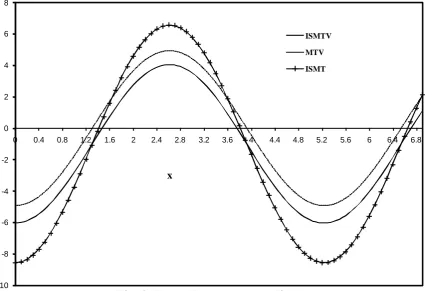
for lowering down the values of displacement component and initial stress causes an increase in the numerical values of the displacement. Fig. 2 represents the variation of normal stress
zz
t
distance x. It attains its maximum values 4.0480, 4.9372 and 6.5564 for ISMTV, MTV and ISMT theories respectively atx
2.6
. Clearly the presence of void parameters and initial stress parameter acts to decrease the magnitude of normal stress.Fig. 3 depicts the variation of temperature distribution
T
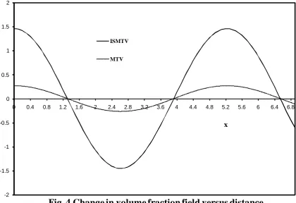
with distance x. The behaviour of temperature distribution is almost opposite in nature for MTV theory as compared to ISMTV and ISMT theories. Effect of initial stress and the presence of voids is to decrease the magnitude of temperature. Fig. 4 shows the distribution of change in volume fraction field
versus x. It shows same trend of oscillatory nature in both the theories ISMTV and MTV but oscillatory nature is more prominent in ISMTV theory as compared to MTV theory.Case 2: Insulated boundary
The variation of normal displacement
w
with distance x is shown in fig. 5. The behaviour ofw
for all the cases is almost similar. It is decreasing in the ranges0
x
2.6
and5.2
x
6.9
and increasing in the range2.6
x
5.2
. Due to presence of voids, the normal displacement componentw
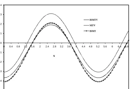
has appreciably decreased and initial stress increases the values of normal displacement. Fig. 6 depicts the distribution of stress componentt
zz versus x. The stress component is also having the similar pattern in all the three cases. It behaves like a decreasing function in the domain2.6
x
5.2
and an increasing function in the domains5.2
x
6.9
and0
x
2.6
. Highest values of stress component for ISMTV, MTV and ISMT theories are 1.8928, 3.0852 and 2.1070 respectively. Clearly initial stress and void parameters are responsible for decreasing the magnitude of normal stress. Fig. 7 represents the changes of temperature distributionT
with distance x. The temperature distribution exhibits the same behaviour in all the three theories. In the domains-0.05 -0.04 -0.03 -0.02 -0.01 0 0.01 0.02 0.03 0.04 0.05
0 0.4 0.8 1.2 1.6 2 2.4 2.8 3.2 3.6 4 4.4 4.8 5.2 5.6 6 6.4 6.8
x
Fig. 5 Normal displacement versus distance
ISMTV
MTV
ISMT
-5 -4 -3 -2 -1 0 1 2 3 4
0 0.4 0.8 1.2 1.6 2 2.4 2.8 3.2 3.6 4 4.4 4.8 5.2 5.6 6 6.4 6.8
x
Fig. 6 Normal stress versus distance
ISMTV
MTV
-0.15 -0.1 -0.05 0 0.05 0.1 0.15
0 0.4 0.8 1.2 1.6 2 2.4 2.8 3.2 3.6 4 4.4 4.8 5.2 5.6 6 6.4 6.8
x
Fig. 7 Temperature versus distance
ISMTV
MTV
ISMT
-0.5 -0.4 -0.3 -0.2 -0.1 0 0.1 0.2 0.3 0.4 0.5
0 0.4 0.8 1.2 1.6 2 2.4 2.8 3.2 3.6 4 4.4 4.8 5.2 5.6 6 6.4 6.8
x
Fig. 8 Change in volume fraction field versus distance
ISMTV
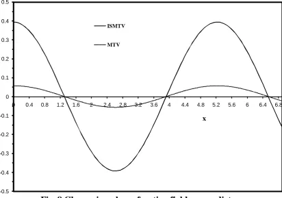
Fig. 8 reveals the variations of change in volume fraction field
versus distance x. It shows similar behaviour in both the theories ISMTV and MTV. It is a decreasing function in the domain0
x
2.6
and5.2
x
6.9
and an increasing function for2.6
x
5.2
. It is clear that oscillatory nature is more prominent for ISMTV theory.7.Concluding remarks
Analysis of normal displacement, normal stress, temperature and changes in volume fraction field due to mechanical load in a semi-infinite generalized initially stressed thermoelastic medium with voids is an interesting problem of mechanics. Normal mode analysis technique has been used which is applicable to a wide range of problems in thermoelasticity. This method gives exact solutions without any assumed restrictions on the actual physical quantities that appear in the governing equations of the problem considered. The results concluded from the above analysis can be summarized as follows:
(i) All the fields are found to be sensitive towards the initial stress and void parameters. Figures indicate that initial stress and void parameters have both increasing and decreasing effects on the numerical values of the physical quantities.
(ii) The values of physical variables are also affected by different boundaries. In isothermal boundary trend of temperature distribution curve for MTV theory is opposite to that due to insulated boundary. Amplitudes of normal displacement are much less for all the theories in insulated boundary as compared to isothermal boundary. The difference between the numerical values of normal stress for ISMTV and ISMT theories is more prominent in case of isothermal boundary than that in insulated boundary. It is found that there is very small difference between the values of temperature for ISMTV and ISMT theories in isothermal boundary as compared to insulated boundary. Thus different types of boundaries significantly affect the problem.
The results obtained as a consequence of this research work should prove beneficial for researchers working on generalized thermoelastic solids with voids. The introduction of magnetic field, initial stress and void parameters to the generalized thermoelastic medium presents a more realistic model for these studies.
References
[1] H.W. Lord, Y. Shulman, A Generalized Dynamical Theory of Thermoelasticity, J. Mech. Phys. Solids, vol. 15, pp. 299-309, 1967. [2] A.E. Green and K.A. Lindsay, Thermoelasticity, J. Elasticity, vol. 2, pp. 1-7, 1972.
[3] M.A. Goodman and S.C. Cowin, A Continuum Theory for Granular Materials, Arch. Ration. Mech. Anal., vol. 44, pp. 249-266, 1972. [4] J.W. Nunziato and S.C. Cowin, A Non-linear Theory of Elastic Materials with Voids, Arch. Ration. Mech. Anal. vol. 72, pp. 175-201,
1979.
[5] S.C. Cowin and J.W. Nanziato, Linear Theory of Elastic Materials with Voids, J. Elasticity, vol. 13, pp. 125-147, 1983. [6] P. Puri and S.C. Cowin, Plane Waves in Linear Elastic Materials with Voids, J. Elasticity, vol. 15, pp. 167-183, 1985.
[7] R.S. Dhaliwal and J. Wang, Domain of Influence Theorem in the Theory of Elastic Materials with Voids, Int. J. Engng. Sci., vol. 32, pp. 1823-1828, 1994.
[8] R.S. Dhaliwal and J. Wang, A Heat-flux Dependent Theory of Thermoelasticty with Voids, Acta Mech., vol. 110, pp. 33-39, 1995. [9] S.C. Cowin, The Viscoelastic Behaviour of Linear Elastic Materials with Voids, J. Elasticity, vol. 15, pp. 185-191, 1985. [10] D. Iesan, A Theory of Thermoelastic Materials with Voids, Acta Mech., vol. 60, pp. 67-89, 1986.
[11] G. Liu, Z. Bu and X. Liu, The Temperature Distribution of a Two-dimensional Thermoelastic Material with Voids, Heat Transfer-Asian Research, vol. 39, pp. 507-522, 2010.
[12] B. Singh, On Theory of Generalized Thermoelastic Solids with Voids and Diffusion, European J. Mech.-A/Solids, vol. 30, pp. 976-982, 2011.
[13] A. Montanaro, On Singular Surfaces in Isotropic Linear Thermoelasticity with Initial Stress, J. Acoust. Soc. Am., vol. 106, pp. 1586-1588, 1999.
[14] P. Ailawalia and N. Singh, Effect of Rotation in a Generalized Thermoelastic Medium with Hydrostatic Initial Stress Subjected to Ramp Type Heating and Loading, Int. J. Thermophysics, vol. 30, pp. 2078-2097, 2009.
[15] B. Singh, A. Kumar, J. Singh, Reflection of Generalized Thermoelastic Waves from a Solid Half-space under Hydrostatic Initial Stress, J. Appl. Math. Comp., vol. 177, pp. 170-177, 2006.
[16] B. Singh, Effect of Hydrostatic Initial Stresses on Waves in a Thermoelastic solid Half-space, J. Appl. Math. Comp., vol. 198, pp. 494-505, 2008.
[17] H. Sherief, K. Helmy, A Two-dimensional Problem for a Half-space in Magneto- thermoelaticity with Thermal Relaxation, Int. J. Engng. Sci.,vol. 40, pp. 587-604, 2002.
[18] H.M. Youssef, Generalized Magneto-thermoelasticity in a Conducting Medium with Variable Material Properties, J. Appl. Math. Comput., vol. 173, pp. 822-833, 2006.
[19] A. Nayfeh, S. Nemat-Nasser, Electromagneto-thermoelastic Plane Waves in Solids with Thermal Relaxation, J. Appl. Mech., vol. E(39), pp.108-113, 1972.
[20] R. Kumar and L. Rani, Mechanical and Thermal Sources in Generalized Thermoelastic Half-space with Voids, J. Pure Appl. Math, vol. 36(3), pp. 113-133, 2005.