Benjamin La Borde
U C L
University College London
England
Submitted for
The Degree of Doctor of Philosophy The University of London
All rights reserved
INFO RM A TIO N TO ALL U SER S
The quality of this reproduction is dependent upon the quality of the copy submitted.
In the unlikely event that the author did not send a complete manuscript
and there are missing pages, these will be noted. Also, if material had to be removed,
a note will indicate the deletion.
uest.
ProQuest 10016709
Published by ProQuest LLC(2016). Copyright of the Dissertation is held by the Author.
All rights reserved.
This work is protected against unauthorized copying under Title 17, United States Code. Microform Edition © ProQuest LLC.
ProQuest LLC
789 East Eisenhower Parkway
P.O. Box 1346
The work concentrates on orthogonal wavelets and documents a generic method for designing discrete wavelets which encompasses the well-documented Haar and Daubechies.
Only wavelets up to 6 taps are considered, these being derived from seed equations capable of explicit solution: higher degrees than this require iterative solution.
Much of the work describes the derivation of the generic method, leading to equations which although comprising simple algebra do become complicated, especially for the 6 tap case, which "reduces" to a single quartic equation of great complexity. The seed equations are the usual ones of orthonormality and moment conditions with the highest moment condition replaced by a generic parameterized "lock" condition which introduces a new degree of freedom not found in the Daubechies wavelets.
Abstract Contents Figures Tables Glossary Acknowledgements Chapter 1 Introduction
1.1 Motivation
1.2 Thesis structure
1.3 Background
1.4 History
1.5 Future
1. 6 Wavelets
1.6 .1 Form and function
1.6 . 2 abc wavelets
1.6.3 Wavelet hierarchy
1.6.4 Vetterli
1.6.5 Szu
1.6.6 Pollen
1.7 Summary
Chapter 2 Continuous wavelets and their influence on discrete wavelets
2.1 Introduction
2.2 The continuous wavelet transform 2.3 Admissibility condition
2.4 Conclusion
Chapter 3 Discrete wavelets and the fast wavelet transform
3.1 Introduction
3.2 Derivation
3.2.1 Daubechies' wavelets
3.3 Implementation
3.3.1 Multiresolution decomposition
3.4 Appearance
3.5 Conclusion
Chapter 4 Derivation of generic 4 tap wavelets
4.1 Introduction
4.2 Seed equations
4.3 Wavelet solution: a step by step derivation
4.4 Verification
4.5 Appearance
4.6 Conclusion
Chapter 5 Derivation of generic 6 tap wavelets
5.1 Introduction
5.2 Seed equations
5.3 Wavelet solution: a step by step derivation
5.4 Verification
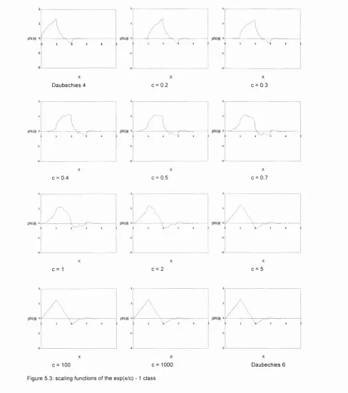
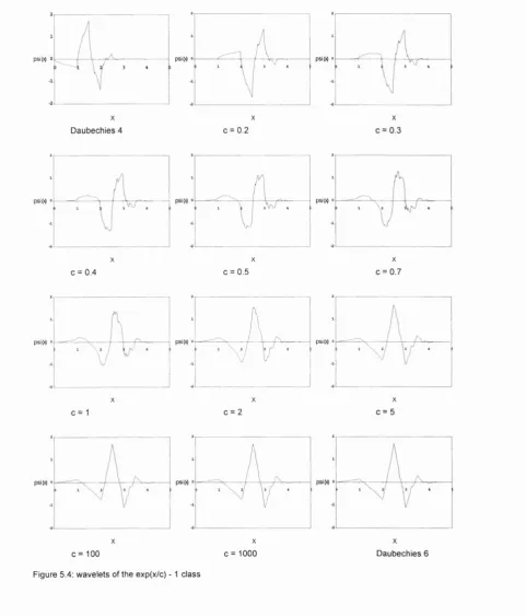
5.5 Appearance
5.6 Frequency response
5.7 Conclusion
Chapter 6 Application of a specific generic 6 tap wavelet, the 8 6
6.1 Introduction
6.2 The fast wavelet, 8 6 6.3 Software implementation 6.4 Computational results
6.5 's place among generic taps
7.2 Top and bottom chirps 90
7.3 Conclusion 96
8 Transient detection 97
8 . 1 Introduction 97
8 . 2 Background 97
8.3 Data description 103
8.4 Practical considerations 105
8.5 Transient location 106
8.5.1 Role of the abc wavelets 106
8.5.2 Test framework 106
8.5.3 Expected results 1 1 1
8 . 6 Locating short transient, tA 1 1 2
8 .6 . 1 Voting system 1 1 2
8 .6 . 2 Decision criterion 113
8.6.3 Results 113
8.6.4 Conclusion 116
8.7 Locating extended transient, tc 116
8.7.1 Voting system 116
8.7.2 Decision criterion 117
8.7.3 Results 117
8.7.4 Conclusion 119
8 . 8 Summary 1 2 0
9 Conclusion 1 2 1
9.1 Overview of the programme of work 1 2 1
9.2 Significant findings 1 2 2
9.3 Future work 1 2 2
Appendix A: Wavelet selection for tA 123
Appendix B: Wavelet selection for tc 126
page 14 1.6.1 2nd paragraph: page 29:
page 31 3rd paragraph: page 43 4.1:
page 43 (4.1):
page 51 first paragraph: page 53 (5.1):
page 54 5.3:
page 77 first paragraph:
change impossible to very difficult
change the deltas equal 1 to the integrals o f the deltas equal 1 change necessary condition to sufficient condition
N-1
change f(x,c) = 0 to i7(~lff(x^,c) = 0
k=0
change orthonormality to normalization change none zero to non-zero
w avel on point A 114 Figure 8.13: transient votes for wavelets c = 0.2,1.0,1000, for w avel on points A and C,
using levels 2,3,4,5, 6 116
Figure 8.14: transient votes for wavelets c = 0.2,1.0,1000, for w avel on point C, using
levels 2,3,4,5, 6 117
Figure 8.15: transient votes for wavelets c = 0.2,1.0,1000, for w avel. Successive
Table 5.1 : tap values for f(x,c) = exp(x/c) -1 73 Table 6.1 : comparative time in seconds of the D6 and B6 transform segments 8 6 Table 6.2: comparative time in seconds of the D6 and B6 transform segments adjusted
for the loop overhead 87
Table 6.3: comparative time in seconds of double addition and multiplication 87 Table 6.4: comparative time in seconds of double addition and multiplication adjusted
for the loop overhead 87
Table 6.5: comparative time in seconds of the full D6 and B6 wavelet transforms 87
Table 6 .6: iterative search for C2 = % 89
Table 7.1 : best wavelet choice for compression of the chirp class
y = top/bottom[sin(exp(6-x/200)/n)], x e [0,1023] 96 Table 8 .1 : wavelet extrema locations for the range of wavelets 0 to 23 112 Table 8.2: t^ results for threshold = 2000 mean vote for the range of wavelets 0 to 23 115 Table 8.3: tc results for threshold = 20 mean vote for the range of wavelets 0 to 23 119 Table A.1
Table A.2 Table A 3 Table A 4 Table A.5
tA results for threshold = 3000 mean vote 123
tA results for threshold = 4000 mean vote 124
tA results for threshold = 5000 mean vote 124
tA results for threshold = 5500 mean vote 125
tA results for threshold = 5550 mean vote 125
Table B.1 : tc results for threshold = 30 mean vote 126
Table B.2: tc results for threshold = 40 mean vote 127
Table B.3: tc results for threshold = 50 mean vote 127
Table B.4: tc results for threshold = 60 mean vote 128
(j), phi scaling function v|/, psi wavelet
affine property of translation and dilation AKA Also Known As
ANN Artificial Neural Net, AKA Neural Net APR Automatic Pattern Recognition
ASSP IEEE Transactions on Acoustics, Speech and Signal Processing CFAR Constant False Alarm Rate
CON Complete Ortho-Normal
EMTP ElectroMagnetic Transient Program (proprietary simulation software) FT Fourier Transform
IEEE Institute of Electrical and Electronics Engineers Inc JPEG Joint Photographic Experts Group
ISAR Inverse Synthetic Aperture Radar MPEG Moving Pictures Experts Group NGC The National Grid Company pic NN Neural Net
SAR Synthetic Aperture Radar
SIAM Society for Industrial and Applied Mathematics SNR Signal to Noise Ratio
SMPTE Society of Motion Picture and Television Engineers SP Signal Processing
SPIE Society of Photo-optical Instrumentation Engineers, AKA The International Society for Optical Engineering
This research was undertaken within the Postgraduate Training Partnership established between Sira Ltd and University College London. Postgraduate Training Partnerships are jointly sponsored by the Department of Trade and Industry and the Engineering and Physical Sciences Research Council. They are aimed at providing research training relevant to a career in industry and at fostering closer links between the science base, industrial research, and industry.
Consequently, supervisors from both UCL and Sira deserve recognition. They are listed here alphabetically by last name so as to offend none.
Dr Mike Cutter, Sira, Kent.
1 INTRODUCTION
1.1 Motivation
This thesis documents the PhD of Benjamin La Borde, started in October 1993 in the Department of Electronic and Electrical Engineering, University College London, England. At commencement the title was simply "Wavelets and the wavelet transform" without remit for specific research direction.
The achievement of this PhD is the development of a generic method for designing discrete wavelets which encompass the well-documented Haar and Daubechies wavelets, and brought them together in a relationship previously unexplored using a single parameter. They are termed the abc wavelets, the name deriving from the use of a single extra parameter, c, in their representation.
The focus on generic discrete wavelets defined with a single parameter was motivated by the fact that the problem was open and that the literature showed no method for closed-form discrete wavelet design modelled by a single parameter.
1.2 Thesis structure
The thesis comprises 9 chapters. This chapter, chapter 1, examines the literature of parameterized and general wavelets, and outlines historical development. The concept of parameterization is put into context with examples of extant systems.
Chapter 2 is an overview of the continuous wavelet transform. It shows how the inverse is calculated and how it depends on the admissibility condition. The importance of admissibility is explained as a necessary condition also in the derivation of discrete wavelets.
Chapter 3 examines the development of discrete wavelets, focusing on Daubechies' wavelets and the fast transform. Readers unfamiliar with the wavelet transform would benefit from an early reading of chapter 3.
Chapters 4 and 5 document the derivation of the generic 4 tap and 6 tap wavelets respectively. Chapters 6 , 7 and 8 concentrate on applications. Each chapter describes a separate aspect of the 6 tap abc wavelets:
Chapter 6 looks at the derivation and implementation of a specific 6 tap wavelet, useful in compression, being similar in quality to Daubechies 6 , but offering a potential speed advantage in implementation.
Chapter 7 considers wavelet selection from the six tap class to optimize compression efficiency. Here the parameter is used to produce a set of wavelets from which the most efficient can be selected.
Chapter 8 illustrates application of the abc class to power system transient detection. Further literature background is presented, and a case study considers the selection of best wavelets for detecting different transient types occurring in the switching state of high voltage relays.
1.3 Background
The use of wavelets has won recent favour in signal analysis due to the advent of digital computing. The father of the subject was Alfred Haar [27], a Hungarian mathematician who devised the first wavelet in 1910. Like the grandfather clock, who's owner died taking the key with him, wavelets fell into disuse with Alfred. The man died.
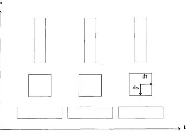
Nothing happened until the 1980's when the French resurrected the subject for use in seismic analysis. In 1984 Jean Morlet [44], a geophysicist, used complex continuous wavelets to provide variable resolution in both spatial and frequency domains. Compared with the conventional Fourier transform (FT), the wavelet provides location information as well as frequency content, and is more useful in analysing signals for which location information is important. The wavelet transform (WT) also has the advantage of automatically adjusting its window size to the resolution of the examining basis. Large scale (low frequency) uses a large window; small scale (high frequency) uses a small window. The concept is borrowed from quantum mechanics which prohibits simultaneous high precision in time and frequency (Heisenberg's principle). This is called a constant Q feature, dm dp > c, for some positive constant c ~ 1 (Kaiser [34]).
The symbol p is used as the signal space parameter to represent time t or distance x, in a generic fashion without reference specifically to either dimension. Similarly, m can be temporal or spatial frequency respectively.
The wavelet constant Q property is shown graphically in figure 1.1 compared with Fourier windowed sampling, figure 1.2. Mallat [40] shows that wavelets have good resolution in both time and frequency. It is the combined properties of constant Q and localization that often leads to the choice of the wavelet transform in preference to the Fourier transform.
0)
Figure 1.1: wavelet transform resolution cells
CO
dco
Finally, the discrete wavelet transform devised by Mallat [40, 51] offers order N complexity, thereby giving a speed advantage over fast Fourier which is itself order N log(N), (Strang [64]). This advantage rightly names Mallat's transform the fast transform. Details are given in chapter 3.
A recent JASON review [31] identified 3 main areas for wavelet application: data compression; de-noising; feature extraction. The growth of wavelet usage is manifested by the wealth of publications and conferences in the last 8 years. The number 8 is chosen, based on a quote of Stéphane Mallat from a 1989 paper [41] in which he thought it necessary to explain the term when introducing "a function Y(x) called a wavelet."
Although much of the published material (about 90%) is from universities and government institutions, wavelets are slowly migrating out of academia and finding applications in commercial video and audio compression, as well as feature recognition in such areas as human signature validation (Tian [72]), machine health monitoring (Atlas [7]) and enhancement of Synthetic Aperture Radar (SAR) images (Tuthill [73]).
The field is still in a state of development with wavelet not yet a word in engineers' vocabularies, and certainly only those people actually engaged in their use know what wavelets are. This is contrary to the ubiquity of the Fourier transform, which even if a person doesn't use it, at least has heard of it. Bracewell [10] discusses the broader aspects of the transform method from the viewpoint of numerical computation.
Despite the advantages cited earlier, the slow uptake is due, in some part, to the simple reason that Fourier analysis does work and is a very useful tool in signal analysis.
1.4 History
Briefly, the significant waypoints in the journey to current theory are outlined by the names below:
CON (Complete Ortho-Normal) periodic CON non-periodic
CON CON
CON beyond Haar
This is a concise historical review which represents the salient points in this field.
Going back to Jean Morlet in 1984/5; he invented the wavelet due to his dissatisfaction with the FT. It was his work which united the mathematicians (about 300 world-wide) with engineers and physicists, thus bringing together theory with application. Working in seismology, he first collaborated with Alexander Grossman. At first no one listened to his theories at geophysics conferences because they weren't in books. Grossman promoted the idea of scale analysis. He was interested in discrete bases but at this time no orthogonal ones existed. This inspired Ingrid Daubechies to pursue compactly supported discrete wavelets. Her major wavelet selling point was the compact energy representation of the WT. She sought to find discrete orthonormal wavelets which at the time were thought impossible, beyond the simple case of the two tap Haar. The property of orthonormality lends a degree of simplification to favour them over non- orthogonal wavelets, namely that orthonormality renders the analysis and synthesis matrices identical. The term identical here implicitly recognizes the transposition of the inverse matrix, there being a one-to-one correspondence of matrix elements.
• Fourier 1880 global
• Haar 1910 local
• Gabor 1942 wavepacket
• Morlet 1985 affine
1.5 Future
Wavelets are good at linear approximation, ie you just add together the contributions from each scale of the approximation. Fourier works the same way but has no sensible connection between scales (frequencies) because no location information exists. New directions for wavelets are adaptive methods and irregular grids, the major qualification being that direction will
be application driven.
In considering image compression, JPEG decays suddenly whereas the WT decays gracefully (Huffman [30]). Sun [65] Illustrates this succinctly in his scheme for image transmission. In adaptive pattern recognition, the challenge is to find the feature vector at an appropriate resolution, taking advantage of the WT's multiresolution analysis. Here also we want graceful degradation (Szu [6 8]).
Time-frequency joint representations traditionally do not use wavelets, and this will probably remain the case, their being better served by windowed Fourier and Wigner-Ville (Pan [49]). Rioul [54] compares the two methods, the wavelet and Wigner-Ville, and examines the role of scale in signal analysis. Automatic Pattern Recognition (APR), based on biorthogonal systems, are another area served well by multiresolution analysis: here the use of neural nets allows graceful degradation, and as Assef [6 ] states, "Artificial Neural Nets can construct relations between input and output data without any explicit analytical model". Whether this is seen as a merit or escape clause, the future is adaptive neural net transforms.
The discrete wavelet transform is chosen for computational efficiency. Wavelets allow you to work incrementally, by only computing those scales necessary for particular analyses. High frequency -> small scale, le scale is opposite to frequency; "a" as in (a, b) is the inverse of ©. The properties of dilation (a) and translation (b) give a new two variable transform coined by the term affine, a concept fundamentally different from frequency. It is the wavelet's affine property which will give it a lasting place in the engineer’s toolbox of tomorrow.
1.6 Wavelets
1.6.1 Form and function
The wavelet method is a branch of information theory concerned with forms of representation. The form of representation used to describe a problem determines the degree of ease or difficulty with which that problem can be solved. As an example, consider dividing 100 by 10. In base 10 it is easy; a simple shift one place right. In base 2 the calculation is more lengthy, but it is still soluble. If, however, Roman numerals are used, the problem becomes impossible. | is not defined. Roman numerals do not support division. To repeat: the system of representation used to describe a problem determines crucially whether the solution of that problem is easy, difficult or impossible.
All the words on this page, and all the pages in this thesis, and all the books ever written can be expressed in only 26 letters. This is an impressive feat for so small an alphabet. Wavelets are the mathematician's alphabet. Wavelets provide efficient descriptions of functions. The wavelet function and the wavelet transform depend for their success on the affine principle. Affine means the process of translation and dilation.
by a parameter 'a', such that as 'a' increases, dilates, and as 'a' decreases, contracts.
The wavelet is a bounded function, and is zero almost everywhere, except for some interval where it has an oscillatory form. The interval over which it is non-zero is called its region of support, or simply its support.
The wavelet transform is an inner product method such that the analysing wavelet is correlated with the underlying signal.
W(a,b) = j f( x ) M /|^ ^ ^ jd x
where W is the wavelet transform of f. (A more rigorous description is given in chapter 2).
W(a,b) is a function of 2 variables, a and b, and thus gives information about size and location. In wavelet terms, size in embodied in the concept of scale, which is the opposite of frequency in Fourier analysis. Large scale compares with low frequency; small scale compares with high frequency. The comparison is not exact since the wavelet is not sinusoidal, due to its finite support.
Thus W(a,b) is a description of f(x) in terms of its similarity with the analysing wavelet. Since W(a,b) is a two parameter transform, it describes f(x) in terms of the dilated and translated wavelet, and so identifies constituent features of the signal in terms of their size and position. This, in Fourier analysis is impossible, because it has no parameter for position.
Implicit in the wavelet transform is the concept of self similarity, such that any wavelet Yai.bi is a self-similar form of any shifted and dilated version of itself, Ya2,b2- Thus the wavelet is size- invariant; able to locate features within signals at any resolution.
Progressing to discrete wavelets, the wavelet transform is implemented as a matrix technique using an "analysis" matrix. Here the wavelet is represented by a small number of coefficients called taps. They take this name to avoid ambiguity with the wavelet transform coefficients, Wg b, which are themselves called the wavelet coefficients. The number of taps within the analysis matrix determines the length of the wavelet, ie the support. Longer wavelets have more taps and can thus respond to more of the signal at once. The disadvantage is that the transform is slower. The discrete wavelet transform is described in chapter 3, where the matrix method of shifting and dilating is explained.
However, one thing which must be brought into this overview is the inclusion of another function, the scaling function, which is a necessary component of the discrete wavelet transform. The scaling function has the symbol phi, and like \j/ is a shifted and dilated function of x:
The reason for having two functions is that \\f and ^ extract different sorts of information from f. (j) is an averaging function which gives a description of the smooth form of f at any resolution. is a differencing operator and contains the fine detail which must be added to (f> to recover the exact form of f at a particular resolution.
1.6.2 abc wavelets
The new class of wavelets described in this thesis is called abc wavelets, first introduced in 1995 (La Borde [35]), and. further documented in 1996 (La Borde [36]). The name is drawn from an extra parameter, c, in addition to the conventional ones of "a" for dilation and "b" for translation: 'F(a,b,c). The abc class is discrete and orthogonal. Explicit solutions exist for 4 and 6 taps. The name abc is used as a simple identifier for these classes, although "a" and "b" are not strictly parameters in the discrete case, both being fixed to 2 for the fast Mallat transform. The name however, is indicative of parameterization and is a useful shorthand for "parameterized wavelets". Full derivation is given in chapters 4 and 5; their introduction here is to establish a name for these wavelets and put a handle on the thesis, as well as to familiarize the reader with the name "abc wavelets". The use of a parameter, c, in the wavelet derivation, leads to generic expressions for the taps, yielding a continuous set of discrete wavelets in a wavelet space defined in terms of this single parameter. To emphasize: the wavelets are discrete; the class is continuous. A particular value of c gives one particular discrete wavelet.
1.6.3 Wavelet hierarchy
Wavelets can be split into two categories: continuous and discrete. Of the discrete version, a further tripartite division exists of orthogonal, non-orthogonal and biorthogonal. Biorthogonal wavelets have advantages over orthogonal ones in that they are symmetric, and therefore better able to represent images because their compressed reconstructions yield less asymmetric distortion. Antonini [5] examines the psychovisual aspects of asymmetric distortion, as similarly does da Silva [17], who also emphasizes the impact of quantization and encoding on image efficiency and distortion.
In this thesis biorthogonal wavelets are not addressed and shall not be discussed beyond this overview. The category of discrete orthogonal wavelets can then be further subdivided into fixed wavelets and parameterized wavelets. The fixed wavelets are a subset of parameterized wavelets, the accepted standards being Daubechies wavelets, so chosen for their optimal smoothness. So dominant are the Daubechies wavelets that some authors describe them simply as wavelets, apparently assuming that there are no wavelets that are not Daubechies. Other times they are referred to as the standard wavelets (Scholl [58]). Following this practice lain out below, in figure 1.3, is a wavelet hierarchy in which the orthogonal wavelets are classed as Daubechies and not-Daubechies. This is a selective hierarchy pruned to show the location of the abc wavelets. Obviously, parameterization is not unique to orthogonal wavelets, and certainly the method exists on other leaves of the tree.
W AVELET
continuous disc rete
non-orthogonal biorthogonal orthogonal
fixed (Daubechies)
parameterized (abc)
Of the parameterized types, there are 3 classes which are covered in this introduction, as a reference to which the abc class can be compared.
They are
• Vetterli • Szu • Pollen
These are 4 and 6 tap wavelets and are documented separately in the following sections.
1.6.4 Vetterli
Martin Vetterli [74, 75] has a four tap wavelet parameterized as (1, a , a , 1). It is not orthogonal
and is stable only for a > 0. It includes asymmetric and symmetric wavelets, including a
quadratic spline for a = 3. Figures 1.4 and 1.5 show a selection of Vetterli wavelets and
corresponding scaling functions for a e [-3, 3].
For negative a the wavelets are unstable, as shown by their high frequency oscillations. This
means that they are unable to model any smooth features of signals, since the wavelets themselves are not smooth. In compression, this would manifest itself as alternate extreme values in the reconstructed signal. In images the effect would appear as neighbouring bright and dark spots throughout the image.
Although the Vetterli class does include symmetric wavelets, this property cannot be exploited due to their instability as illustrated in these figures. Another drawback is their inconsistent area due to unbounded sum of the taps. As explained in chapter 4, the area conservation requirement states
Co + C l + 02 + C3 = a/2
which is clearly untrue for
Cq= 1 Ci = a C2 = a
C3= 1
PsiW
2 3 0 I 2 3 0 1 2 3
(X — 3.0 a = -2.5 ot — 2.0
psiM 0
3 2
psiM
a = -1.5 ot — 1.0 a = -0.5
psiW 0 psiW PsiM
X
a = 0.0 a = 0.5 a = 1.0
X X X
a = 1.5 a = 2.0 a = 2.5
psiM
X
a = 3.0
0 1 2 3 2 3 0 1 2 3
a = -3.0 a = -2.5 a = -2.0
3
0 0 1 3
phiW
a = -1.5 a = -1.0 ot — 0.5
phM 0
X
a = 0.0 a = 0.5
X
ot = 1.0
a = 1.5
-300000
-SQQOO
X
a =2.0 a = 2.5
phiM
X
Ot — 3.0
1.6.5 Szu
psi«
X 1 3
psi«
-mo
a — 3.0 a = -2.5 a = -2.0
psiW 0
psiM 0 psi (4
xoo 1000
-aooo
0 1 2
a = -1.5 a = -1.0 ot — 0.5
3000
lOOO psiW 0
-1000
-3000
T V ,
psiM “ PSi«
X
a = 0.0 a = 0.5 a = 1.0
P S I M 0 psiM «
XOOGO
psiM 0
a = 1.5 a = 2.0 a = 2.5
psi«
X X
a = 3.0 a = 4.0
Figure 1.6; Szu wavelets (1, a , p, 1 ) with p = 3 - V3
2 3 1 2 3
phiW
m x>\
a = -3.0 a = -2.5 ot — 2.0
phM 0 Phi« 0
a = -1.5 ot — 1.0 a = -0.5
sooo
nK M n
-- - . . . > prip9
) 1 2 B
-5000
> 1 2
a = 0.0 a = 0.5
X a = 1.0
X
a = 1.5
phM 0
phiM 0
a = 2.0
a = 3.0 a = 4.0
Figure 1.7; Szu scaling functions (1, a, p, 1 ) with p = 3 - V3
300000
a = 2.5
X
-30000000
1.6.6 Pollen
David Pollen [14, 50] has a 6 tap wavelet, and like Szu uses two parameters, a and p to
characterize his space. The 6 taps are expressed as; Co = [(1+cosa+sina)(1-cosp-sinp)+2sinpcosa]/4 Ci = i(1-cosa+sina)(1+cosp-sinp)-2sinpcosa]/4 C2 = [1+cos(a-p)+sin(a-p) ] / 2
C3 = [1+cos(a-p)-sin(a-p) ] / 2 C 4 = 1 - C 0 - C 2
C5 = I-C1-C3
with a , p e [ - 7 i , 71) .
This is a very versatile system embodying 4 and 6 tap solutions for particular values of a and p. It includes stable and unstable solutions and is always orthogonal. The use of two parameters prohibits comprehensive illustration of Pollen's wavelets; to demonstrate their range, one parameter is set while the other is varied. Figure 1.8 shows the 4 tap case with p = 0 and a selection of values for a. Without deriving their forms, let it be quoted here that for this value of p, Co and C5 are both zero, thus yielding a four tap solution. However there are also non-wavelet solutions, occurring for a = n7i/2 . These are not shown since they are simply straight lines Vj/(X) s 0.
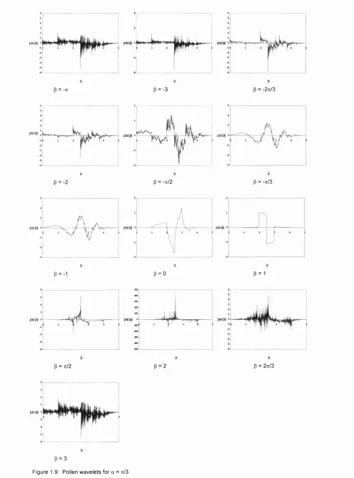
Figure 1.9 shows the full 6 tap case with a set to n/3 while p is varied. This is primarily a six tap
class, although this range does also include some 4 tap solutions, and also the trivial non solutions v|/(x) s 0 already mentioned. The wavelet space covered by this two parameter set embodies the maxim that there are an infinite number of wavelets, most of which have little value. The use of two parameters leads to some difficulty in selecting appropriate values for
psiM PsiM J , r - ^
-■ •
psiM
a = -3 a = -2
psiM “
X X X
cx 7t/3 a = -1 a = -0.5
X X X
a = 0.5 a = 1 a = ïï/3
psiM
X
a = 1.5 a = 2 a = 3
P = -7t P = -3
PsiM
X X
X
p = -271/3
psiM
X
psiW
P = - 2 p = -7t/2
X
p = -7t/3
psiM
X X
p = -1 P = 0 P = 1
psiM psi(x)
p = 7t/2 P = 2 P = 27t/3
psiW
X
P = 3
Gene Tagliarini [69] shows that the Pollen parameters can be searched in algorithmic fashion to find close approximations to desired wavelets. He finds solutions for close approximations to Daubechies wavelets. For the 4 tap Daubechies wavelet, the Tagliarini-Pollen parameters are
a = 1.570887, p = -1.047168 (ie the exact solution is a = n/2, p = -tt/3). In this case C4 and C5 are zero and are not used. His values for Daubechies 6 approximation are a = 1.360035 and
p = -0.783036 (these look seductively close to a = 3n/7 , p = -ti/4, but this is misleading: these convenient pi multiples do not yield the desired Daubechies 6). Figure 1.10 shows the Tagliarini- Pollen-Daubechies 4 and 6 tap wavelets.
a = 1.570887, p = -1.047168 a = 1.360035, p = -0.783036
1.7 Summary
The background given here shows that wavelet parameterization is a plausible pursuit and that extant systems address the problem with various degrees of sophistication. The following chapters show that a system of wavelets can be derived from first principles to yield 4 and 6 tap analytic classes which always have all of the following properties;
• closed form solution for the taps • orthonormality
• stability
• single parameter • purpose
CONTINUOUS WAVELETS AND THEIR INFLUENCE ON DISCRETE WAVELETS
2.1 Introduction
Although this thesis concentrates on generic discrete wavelets, the continuous wavelet transform is documented here to illustrate an important relationship between continuous and discrete wavelets and to highlight a constraint imposed by the former on the latter. This constraint is called the admissibility condition and derives from a requirement of the inverse transform which states that continuous and discrete wavelets both have no dc component, ie that they integrate to zero. Without this condition there would be little justification in calling discrete filters 'wavelets' other than their having affine properties.
2.2 The continuous wavelet transform
The following description comes from Daubechies' "10 Lectures on Wavelets" [18], expanded to include intermediate steps in the derivation to give an easier progression to the conclusion, namely that ^ (0 ) = 0, ie \\i{x) dx = 0. This is another way of saying the wavelet has no area.
We start with the affine definition of a wavelet
4 ^ ’'’(x) = |ar“ v ( ^ ] (2 .1)
where i® the mother wavelet and '¥‘ '’{x) is the (a,b) member of that wavelet family, also called the daughter wavelet. Parameters a and b are respectively the coefficients for dilation and translation. For the remainder of this analysis the (a,b) superscript will be dropped. In the following discussion, overbar ( ) denotes the complex conjugate. The wavelet transform is denoted tilde (~) and is defined as the inner product of the signal f(x) and the wavelet.
f(a,b) = |a|'^ j" f(x )\j/|^ -^ ^ ^ jd x (2 .2 )
Given the wavelet definition and its transform, we must now engage in some foresight to derive the inverse transform, and in so doing also discover the zero area constraint on the wavelet. The following equation comes from Daubechies book, page 24, and the reason for using it as a starting point is simply that it gives the required result. For algebraic simplicity the shorthand i is adopted for the integral which otherwise has no name.
00 00
I =
j J
^ f(a ,b ) g ( a ,b )d a d b (2.3)Substitute in the wavelet definition for f and g to give
00 00
The next step is to express f(x) and g(x) as the inverse Fourier transform of their Fourier transforms. The Fourier transform is denoted hat (*).
^ = 1 1 >K9)e^<^")d9
—00 —00 —GO —00 J ^ —00
— 0 0 — 0 0 J ( — 0 0
Exploiting the Dirac delta equivalence
00
A j Q±i\^(jiZ = 8{\L)
The I components above simplify as
J d x e ““^ e K ^ ) = | d x e “K ^“l] e '® a = 2 7 i e '® i Ô
and
^ Û \ for^, V 3y
J d y e ^ ‘^^'e“K ^ ) = J d y e K ^ '‘ ¥ ]e ^ ® i = 2 7 te ^ ® i
fo r
6 6'
Then the deltas equal 1 when ^ = — and . With these simplifications the integral becomes
a a
00 00
= 2n J dSf(S)g(S)v(aS*(aS)
= 2 n j d%f(%)g(^)j ^ | v ( a % f
Now use the variable substitution u = a^.
00 00
1 = J d ÿ ( | ) i ( I ) . 2 n j ^ l v ( u ) f
=
< f,g >
where
(2.3) now yields
I =
J J
-^f(a ,b )g (a ,b ) da db = <f,g:ie
1 1I
dy g(y)|a da db = <f,g>Then
J J - ^ f ( a , b ) ' J
dyg ( y ) v ( y )
da db = <f,g>by virtue of (2 .1).
Independence of the integrands allows rearrangement:
j J j
^ ^ f ( a , b ) v |/ ( y ) g ( y ) d y = C^<f,g: —00 —00—00Therefore, by the definition of the inner product, <f,g> =
J
f(x)g(x) dx, the identity becomesJ J ^^f(a,b)v(x)=C,,f(x)
(2.4)Where is the reconstruction constant and x has replaced y to adopt the more common notation.
Rearranging in terms of f(x) we get
f(x) = C;,^J J ^^f(a,b)i|/(x)
(2.5)2.3 Admissibility condition
The start of this chapter justified the inclusion of continuous wavelets by necessity of the admissibility condition, which can now be defined. Validity of the resolution of identity, (2.5), requires that the reconstruction constant is finite.
Therefore it is required that 00
271 J ^ |v f r ( u ) |^ < 00
—00
and since u ranges over [-oo, oo] then a necessary condition is that vj/(u) = 0 when u = 0 to avoid a logarithmically divergent contribution to the integral in the neighbourhood of u = 0 .
Ie vJ/(0) = 0. This is equivalent to stating J \\f{x) dx = 0.
Thus the derivation of the continuous wavelet inverse transform imposes an extra constraint on the wavelet, which although very simple is also very necessary. It Is the invertability of the wavelet transform, (not the wavelet, nor the forward transform itself) which imposes this admissibility condition.
2.4 Conclusion
DISCRETE WAVELETS AND THE FAST WAVELET TRANSFORM
3.1 Introduction
This chapter documents 3 aspects of discrete wavelets: their derivation; implementation, and appearance. The wavelet transform used as the basis of this thesis is the Fast transform, or Mallat transform, known for its speed in transforming signals into their dyadic components in a logarithmically fast manner, such that for an N stage transform, the last N - 1 stages take the same computation time as the single first stage. Thus a doubling of the signal only leads to a doubling of the wavelet transform time, compared with the Fourier equivalent which would require a squaring of the time (Strang [64]), in this case four times the computational time. The fast wavelet transform is a matrix method which offers an additional advantage in that the matrix is inverse self-transpose, which means that the inverse transform is simply a reversal of the forward transform; thus the numerical implementation requires a single function for both the forward and inverse operations.
3.2 Derivation
The transform matrix contains the wavelet taps in line pairs in diagonal form, each line pair representing the scaling function above and wavelet below. This pairing places a size constraint on the matrix, the effect of which is to limit the number of taps, N, to be a multiple of 2, ie an even number. The term "tap" is used to avoid the ambiguous term "coefficient" which is generally reserved to describe the transform values. These taps are themselves not the wavelet, but instead form what is called the pre-wavelet (Stollnitz [61]), or simply the taps. The diagonal construction introduces the translation aspect. Dilation is implemented in the transform by vector decimation after successive matrix multiplications. The term "decimation" is peculiarly hijacked by the wavelet community to mean the removal of alternate components of the signal, ie reducing the signal resolution by a half.
For an N order matrix, N/2 orthonormality conditions guarantee perfect reconstruction when compression is not used, and N/2 equations remain for specifying the desired wavelet characteristics. Classically the moment conditions are used to provide polynomial accuracy of degree N/2 -1 (Strang & Fix [62]).
Daubechies wavelets are the industry standard for signal compression. Their use in Mallat decomposition is based on these conditions of orthonormality, supplemented with N/2 moments, also known as Strang accuracy conditions [63]. The discrete wavelet technique depends on the success of the Daubechies wavelet matrix form which in addition to being inverse self transpose, also amazingly offers degrees of freedom. The surprise comes from having N/2 degrees of freedom in a system of N equations in N variables.
It is this freedom that allows the derivation of wavelet families from what othenvise would simply be a system of N equations and N unknowns with a single solution for the matrix transpose. In video compression, the crucial aesthetic factor is smoothness of the synthesized image. The smoothness gained from Daubechies wavelets is clearly essential for perceptive quality, where regularity is more important than accuracy (Morris [45]).
Given a matrix A, A’^ = A^ iff A is orthonormal. Thus the two matrices are A^ = A'^
cO c1 c2 c3 cO -c3 c2 -c1'
c3 -c2 c1 -cO c1 c2 c3 cO
cO c1 c2 c3 c2 -c1 cO -c3
c3 -c2 c1 -cO c3 cO c1 c2
cO c1 c2 c3 c2 -c1 cO -c3
c3 -c2 c1 -cO c3 cO c1 c2
c2 c3 cO c1 c2 -c1 cO -c3
c1 -cO c3 -c2 c3 cO c1 c2
Orthonormality conditions yield: Co^ + c / + Cz^ + Cs^ = 1 and
C2C0 + C3C1 = 0
Additionally, the first two moment conditions yield C3 - C2 + Ci - Cq = 0
and
OC3 - IC2 + 2 ci - 3Co = 0 Solution gives
_ I + V3
472 _ 3 + V3
4 V2 3 —V3
Ci =
0 2 =
C3 = 4 V2 I - V 3
4 V2
This is Daubechies 4; it is the most compact of a sequence of wavelet sets. For N coefficients there are N/2 orthogonality requirements and N/2 moment equations (Amaratunga [3]). This derivation is explained further by considering the scaling equation.
Given a scaling function
4)(x) = Co(|)(2x) + Ci(f)(2x-1) + C2(|)(2x-2) + C3(|)(2x-3)
then it is necessary to have a wavelet of the form
simply because no other arrangement yields a flexible orthonormal system. There are other orthonormal systems, but none with any degrees of freedom, so they all reduce to the trivial case.
Examples follow. Consider a system of just (|)(x) and no v|/(x); then the system becomes
A A^ = A'^
cO cl c2 c3 cO c3 c2 cl
cO cl c2 c3 cl cO c3 c2
cO cl c2 c3 c2 cl cO c3
cO cl c2 c3 c3 c2 cl cO
c3 c2 cl cO
c3 c2 cl cO
c3
c2 c3 cO cl cO
cl c2 c3 cO cl cO
So for orthonormality the conditions are Co^ + Ci^ + + 0 3 ^ = 1
CqCi C')C2 C2C3 — 0 C2C0 + C3C1 = 0
C0C3 = 0
suppose Co = 0 , C3 5* 0 , then Ci = C2 = 0 =>C3 = 1 and the transformation matrix is
0 0 0 1
1
1
1
1
1 0
So the solution is a set of Diracs, (|)(x) = C3(j)(2 x-3)
<t>(x) ij)(2x) (j)(3x) (|)(4x)...
Now suppose C3 = 0, Co 5^ 0,
therefore = C2 = 0 , Cq = 1 and the transformation matrix is
1
1
1
1
(|)(x) = Cq^{2x). Again there are no degrees of freedom, and also the Dirac approximations are collocated, so the system could only model a single point within a signal
4)(x) = Cq(1)(2x) = Cq(|)(4x) = . . . Co4)(2"x).
Another example to consider does use a wavelet of the form
Y(x) = C3(j)(2x) + C2<1)(2x -1) + Ci<|)(2x-2) + Co<J)(2x-3)
and the transformation matrix is
A A^ = A'^
cO cl c2 c3 cO c3 c2 cl
c3 c2 cl cO cl c2 c3 cO
cO cl c2 c3 c2 cl cO c3
c3 c2 cl cO c3 cO cl c2
cO cl c2 c3 c2 cl cO c3
c3 c2 cl cO c3 cO cl c2
c2 c3 cO cl c2 cl cO c3
cl cO c3 c2 c3 cO cl c2
so for orthonormality the conditions are Co^ + c / + C2^ + 0 3^ = 1
C3C0 + C2C1 = 0 CiCq= 0
C3C1 + CgCg —0
[2] Ci = 1, Co = C2 = C 3=0
1
1
1
This yields Diracs displaced by unit interval
which is in fact usable, but yields a tautology: f(n) f(n) which is not attractive for signal analysis nor compression because it can only model the signal as itself!
So (|)(x) and v|/(x) are necessary in their unique forms:
(j)(x) = Co<l)(2x) + Ci(|)(2x-1) + C2<t>(2x-2) + C3(|)(2x-3 ) for the scaling function and
vj/(x) = C3(|)(2x) - C2<|)(2x- 1 ) + Ci(|)(2x-2) - Co(|)(2x-3) for the wavelet.
This is the only form which yields orthonormality in only 2 equations; thus leaving 2 further equations free for conditions such as Strang's or others.
3.2.1 Daubechies' wavelets
The best known wavelets for compression are the Daubechies wavelets. 4 tap wavelets are commonest for fast applications, being simplest to implement; they also offer the advantage of sharp edge representation due to lower impact of local neighbourhood influence.
The Daubechies N wavelet uses the N/2 free conditions for accuracy. These accuracy conditions guarantee polynomial approximation to order N/2 - 1, ie 4 tap wavelets yield polynomial accuracy order 1; 8 tap wavelets yield polynomial accuracy of order 3, and so on. They are ascribed the notation D<N>, eg D4, D6 , DB and so on.
The complexity of the matrix solution means that wavelets of order only up to 6 can be solved analytically. For higher orders iteration is required.
The accuracy condition general form (Cohen, Vial & Daubechies [16]) is
n-1
For 4 tap wavelets, the 4 conditions are: Co^ + c / + 0 2^ + 03^ = 1
C0C2 + C3C1 = 0 C3 - C2 + Ci - Co = 0 -C2 + 2 ci - 3cq = 0
The first two equations ensure orthonormality. These conditions alone guarantee perfect reconstruction. The second two equations are the moment conditions for polynomial accuracy. Complete solution is the tap set
1 ± V 3
Co =
Ci =
a4i
3 ± V s
4V 2
_ 3 + V 3
472
_ I + V 3
472
with the particular solution
I + V3 Co =
Ci =
C2 =
C3 = 4 V2 3 + V3
4 V2 3 - V3
4 V2
l - V J
4 V2
known as the D4. This is the minimum phase 4 tap wavelet, described by Daubechies as "the least asymmetric", so chosen from the two possible solutions for its property of introducing less asymmetric distortion in reconstruction (Walden [77]).
So ubiquitous are Daubechies' wavelets that they have come to be known as "The Daubechies wavelets"; the possessive apostrophe dropped to make Daubechies an adjective, thus: Daubechies wavelets.
3.3 Implementation
3.3.1 Multiresolution decomposition
The technique of multiresolution decomposition comes from Mallat [40] and is based on the transpose self-inverse matrices for forward and backward transformations previously described. Given a signal vector, y, and the tap matrix, A, a single step in the wavelet transform is represented as y Ay.
Repeated quadrature application of the wavelet transformation serves to shuffle and order the coarse and fine elements (the smooth and detail). At each step, the smooth elements are moved to the top of the vector and the subsequent transformation acts only on these elements; a successive halving of coefficients per step. The process continues until dim(A) = N. By necessity then, y must be of length 2"'", for some positive integer M such that 2"'" > N. These are details of implementation and do not affect the discrete wavelet method. A practical description of Mallat's implementation can be found in Numerical Recipes [51].
Let Tp represent a transformation of multiplication by the wavelet coefficient matrix, which itself intrinsically shuffles the elements. This vector is then ordered into its smooth and detail components. The terms smooth and detail refer to the signal scale, which in Fourier terms correspond to low and high frequency terms respectively (Jawerth [32]).
The dyadic transform is demonstrated by the following example in which the signal y has 16 elements.
Successive results in the filter sequence are denoted by bold and italic fonts.
f y i 1 [sll fsll f s i l f s i l [sil [s i]
| y 2 1 |dl| 1 8 2 1 | D 1 | | S 2 | |Di| |S2|
| y 3 1 |s2| |s3 I | S 2 | | S 3 I I 5 2 1 |d i|
| y 4 1 |d2| |s4| | D 2 | | S 4 | \D2\ |D2|
| y 5 1 IS3 I I s5 I | S 3 | |d i| |d i| |d i|
| y 6 1 |d3 I jsej | D 3 | | D 2 | | D 2 I | D 2 1
| y 7 | T i s |s4| o r d e r j s7 j Tg | S 4 | o r d e r j D3 j T4 |D3| o r d e r j D3 j |y8 |-> |d4| -> |s8| -> | D 4 | | D 4 | | D 4 | | D 4 |
|y9 1 |s5| |dl| |dl| |dl| |dl| |dl|
|ylO| |d5| |d2| |d2| |d2| |d2| |d2|
|yii| |s6| |d3 1 |d3| |d3 1 |d3 I |d3 I
| y i 2 | |d6| |d4| |d4| |d4| |d4| |d4|
| y i 3 | 1 s7| |d5| |d5| |d5| |d5| |d5|
|yl4| |d7| |d6| |d6| |d6| |d6| |d6|
| y i 5 | |s8| |d7| |d7| |d7| |d7| |d7|
| y l6| |d8| |d8| |d8| |d8| |d8| |d8|
L J L J L J L J L J L J L J
Quadrature filter process
The final vector is the discrete wavelet transform of the signal y. It can be compressed by setting to zero so many of those coefficients with small moduli. Wavelet compression is an effective technique because most of the signal's energy is represented by a small number of the transform coefficients (Murenzi [46]).
3.4 Appearance
As mentioned in section 3.2, the wavelet taps are not the wavelet itself; instead they are the matrix representation of the filters used in the transform described above. To see the wavelets themselves it is necessary to iterate the dilation equation until the intermediate interval size gives sufficient resolution. By the nature of difference relations, the wavelet can never be drawn exactly since it has no closed form expression. Similarly for the scaling function.
An excellent example of this process comes from Newland [47]. The C code for viewing wavelets was developed from his book. Again, for simplicity, the 4 tap wavelet is illustrated. The
method generalizes for higher orders; further examples are given in chapters 4 and 5.
The wavelet is derived by starting with the scaling function dilation equation. This is also known as the auxiliary equation (Waagen [76]) since it is used to generate the wavelet.
4(x) = Co(t)(2x) + Ci(|)(2x-1) + C2(|)(2x-2) + C2^{2x-3)
Then each approximation (|)j is used to calculate the approximation (j)j+i of the next step.
4)j+i(x) = Co(|)j(2x) + Ci(f)j(2x-1) + C2<f)j(2x-2) + C3<t)j(2x-3)
At each iteration the x interval decreases by a factor of two. As ] increases, the scaling function converges asymptotically to its limiting shape as shown in figure 3.1.
The wavelet is calculated similarly using the same coefficients, reversed and with alternating signs as explained in section 3.2.
v|/(x) = C3(j)(2x) - C2(1>(2x-1) + Ci(|)(2x-2) - Cq^{2x-3)
The wavelet so developed is shown in figure 3.2. This recursion method applies for any wavelet; for this illustration the Daubechies 4 wavelet is shown.
p h i« 0
X X
step 1 step 2 step 3
X
p hl« 0 phiM 0
Step 4 step 5
X X
step 7 step 8
Figure 3.1; recursive development of the Daubechies 4 scaling function
X
psiM ®
X
J=U
X
step 1 step 2 step 3
X
X X
step 4 step 5 step 6
X X
step 7 step 8
Figure 3.2; recursive development of the Daubechies 4 wavelet
X
3.5 CONCLUSION
This chapter has introduced the accepted method of implementation of the discrete wavelet transform for the well-known Daubechies wavelet, explaining the interdependence between the wavelet and the transform; and the necessary conditions on orthogonal wavelets in terms of their matrix representation.
4 DERIVATION OF GENERIC 4 TAP WAVELETS
4.1 Introduction
This chapter looks at the novel technique for designing 4 tap generic wavelets. Based only on orthonormality and constant approximation, the technique exploits the degree of freedom in discrete wavelets when the first moment condition is abandoned. Classically for 4 tap wavelets, the moment conditions provide polynomial accuracy to degree 1, ie constant and linear approximation. For generic derivation the linear moment condition is repiaced by a general lock condition f(x,c) = 0. This concept is explained more fuiiy in chapter 5 when generic 6 tap wavelets are described, and a correspondence made with the Daubechies wavelets in terms of this lock condition. The purpose of this chapter is to introduce the concept of generic taps with the simplest example, ie that of 4 taps. Suffice to say here, the replacement of the linear moment by a parameterized function yields a variable solution for the taps. The term "lock condition" is used as being indicative of the fact that if a particular signal does indeed include this function as an explicit feature, then the wavelet transform will "lock" on to it by giving a zero response for the wavelet and a non-zero response for the scaling function.
4.2 Seed equations
The term "seed equation" is used to embody the sense of a starting point for the derivation. The constant moment is included implicitly in these seed equations as demonstrated below.
There are four design equations.
Cq^ + c / + 0 2^ + Ca^ = 1 orthonormality (4.1)
Co + Ci + C2 + Ca = V2 area conservation (4.2)
Ca - aC2 + pci - yCo = 0 lock condition (4.3)
C0C2 + CiCa = 0 orthogonaiity (4.4)
A simple rearrangement gives a form which is easier to solve. Ignoring for the moment the lock condition,
Co^ + c / + Cg^ + Ca^ = 1 (4.1)
Co + Cl + 0 2 + C3 = V2 (4.2)
C0C2 + C1C3 = 0 (4.4)
(4 .1 )2 ^
(Cq + Ci + C2 + Ca)^ = 2 muitiply out
2 (CoCi + C0C3 + C1C2 + C2C3) = 1 ie (Co + C2)(Ci + 0 3) = %
The only solution is Cq + C2 = Ci + C3 = ^
then
C3-C2 + C i-C o~ 0
which satisfies the constant moment condition as an additional benefit. Then the system of design equations becomes:
Co + Ci + C2 + C3 = V2 (4.2)
C3 - aC2 + pci - yCo = 0 (4.3)
C0C2 + C1C3 = 0 (4.4)
C3 - C2 + Ci - Co = 0 (4.5)
Thus the quadratic form (4.1) has been replaced by a linear equation, facilitating solution of (4.2) to (4.5) by standard row elimination.
4.3 Wavelet solution: a step by step derivation
The system of equations is now
Co + Ci + C2 + C3 = V2 area conservation (4.2)
C3 - aC2 + pci - yCo = 0 lock condition (4.3)
C0C2 + C1C3 = 0 orthogonality (4.4)
C3 - C2 + Ci - Co = 0 linear moment (4.5)
Solution for Co, Ci, C2 and C3 proceeds systematically, starting with the elimination of C3: (4.5) =>
C3 = C2 - Ci + Co (4.6)
Use (4.6) to eliminate C3 from (4.2), (4.3) and (4.4). Substitute (4.6) into (4.2)
Co + Cl + C2 + (C2 - Ci + Ci) = V2
C 2 = : j f - C o (4.7)
Substitute (4.6) into (4.3) C2 - Cl + Co - aCz + pci - yCo = 0
Co(1 - y) + Ci(P -1 ) + Cz(1 - a ) = 0 (4.8)
substitute (4.6) into (4.4) C0C2 + Ci(C2 - Cl + Co) = 0 C0C2 + C1C2 - c / + C0C1 = 0 C2(Ci + Co) = Ci(Ci - Co)
c2=.E<21z£!) (4.9)
Cl + Co
C3 has been eliminated from (4.2), (4.3) and (4.4) to give (4.7), (4.8) and (4.9). Now use (4.7) to eliminate C2 from (4.8) and (4.9).
Substitute (4.7) into (4.8)
Co(1 -y ) + C i(P -1) + (1 - a ) ( ^ - Co) = 0
Ci(P - 1) = ( 1 - a)(Co - ^ ) + Co(y -1)
Co(1 a + Y 1) -
---a - 1
Co(y - a ) +
c , (4.10)
Substitute (4.7) into (4.9)
1 _ Ci(Ci - Co)
—f= - - Co
—---V2 Cl + Co
~ Co)(Ci + Co) = Ci(Ci - Co)
+ - G0C1 - Co + C-|Co ~ 0
C o ' - ^ + c , f c , . ^ l = 0 (4.11)
CO ,
c o ( r - a ) . ^ ) r , \ g - 1 ^
p - l p - l V Ï = 0
multiply out
? go
(
:o (Y -g ) _________ 2co(Y-a)(g-l) \ Vz / ) ( y ~ « ) g - 1
V2 ( p -1)^ Vz ( p -1)^ ( p -1)^ V2(p -l) 2(p -l)
^f2{y - a){a - 1) a - y 1
= 0
1 + ( Y - g )
2^
+ Co
( p _ l) 2 V2(p -l) V2 I 2 ( p - l) ^ 2(p -l)
(p-i)
tidy up this quadratic in Cq
4
*t e) I+
^
- jr
3iw) I
note that the last term = “ M P i) _ g p p - i
then the quadratic becomes
p - i p - i
1 +
solve by the quadratic formula:
J 2 { y
-(P
1 + Y -g
P - l
use a common denominator (p-1) throughout to aid cancellation:
2(Y-gXl-g)+(P-l)^-(P-lX“ -Y)_^ |j2(Y -g)(g-l)+(p-lX g-Y )“ ( p - . f T , (p -l)2+(Y_g) 2 i a-1 fa-P^l V 2 (p -lf 1 1 V2(p-1) j 1 ( P -l)' l2 (P -l)U -ljj
2 ( p -l ) ^ +(Y-g)^ I (P -l)'
J
(p -l) 2 + (y_„)2'
The (p-1)^ term cancels from the denominator of each term in the numerator and denominator of the whole expression
2(y-aXl-a)+(P-l)^-(p-lXa-Y)±V2 j^V 2 (Y -a )(a -l) + ^ ^ ^ -2|(p~l)^+(Y-a)^j(a-lXa-p)
2V2[^(p-l)2+(Y-a)2j
Now, to simplify further progress use a shorthand notation and express Cq as where L is the left hand term; S is the square root term; and D is the denominator, thus:
< = 0 = 4 ^
where D = 2>/2[^(p-1)^ + (y - a)^j
and L = 2(y - a)(1 - a) + (P -1)^ - (p - 1)(a - y)
= 2y - 2ay -2a + 2a^ + P^ - 2p + 1 - ap + Py + a - y L = 1 - a + 2a^ -2p - aP + P^ + y - 2ay + Py
The square root term is S = V I | | v2 (y -« ) ( « - !) + -2{(p -i)^ + (Y-a)^}(a-i)(a- p)
take the V I inside the square root and multiply out.
S = { 4 ( y - a ) V l) ^ + 4(Y-«)(a-1)(|3-1)(a-(')'4(T-a)(a-1)(p-1)^ + (P-1) V ^ ) ^ - 2 (P-1)’ (a-y) + (p-1)" .4(p-1)^(a-1)(a-P).4(T.af(a-1)(a-P)}%
collect the (1-p) terms inside the square root
S = {(1-prt-4(y-a)(a-1) + (y-a)^ + 2(1-p)(a-y) + ( P - l f - 4(a-1)(a-P)] + 4{y-a)^(a-1)^ - 4 (y-af(a-1)(P -1) - 4 (y-af(a-1)(a-p )}^
S = {(1-P)^[4(a-1)(a-y+p-a) + (a-y)(a-y+2-2P) + ( P - lf ] + 4(y-a)^(a-1 )(a-1 -P+1+p-a)}^ Now take the (1-P)^ outside the square root and multiply out:
Using Cq = Cq now becomes:
result:
_ 1 - a + 2 a ^ - 2P - a P + + Y - l a y+ Py ± ( l - p ) ^ 1 + 2 a + - 6p + 2 a p + + 2 y - 6 a y + 2Py +
Cn —
---272(^(l-p)2 + ( y - a )2j
Given Cq, Cg is now derived using (vi), Cg = ^ - Cg
Then C2 ~ —?=- — V2
1 - a + 2 a ^ - 2p - aP + p^ + y - 2ay + Py ± (l - p)-J 1 + 2 a + - 6p + 2ap + p^ + 2y - 6ay + 2Py + y^
2>/2[^(l-p)^ + (y-a )^ j
use a common denominator
C 2 =
2 [ ^ ( l- p ) ^ + ( y - a ) ^ j - l + a - 2 a 2 + 2p + a p - p 2 - y + 2 a y - P y T ( l - p ) ^ l + 2 a + a 2 - 6 P + 2aP + p2 + 2 y - 6 a y + 2Py + y"
2V2{^(l-p)^ + ( y - a f j
2^1 - 2p+ p^ j+2^y^ - 2ay+ j - 1 + a - 2 a ^ + 2 p + a P -P ^ - y + 2ay - Py T (l - p )y l+ 2 a + a ^ - 6p + 2ap+p^+ 2y - 6a y + 2Py+ y^
2>/2^ ( l - p ) 2 + ( y - a f j
result:
_ l + a - 2 p + ap + p ^ - y - 2 a y - P y + 2 y ^ T ( l - p ) ' / l + 2 a + a ^ - 6p + 2aP + p^ + 2 y -6 a y + 2 P y + y^ 0 2 -
---272^(l-p)2 + (y-a)2j
Also, given Cq, the expression for Ci can be found using (4.10):
. . a — 1 c o ( y - a ) + — ^
F T ^
Again, to reduce complexity, adopt the shorthand for the square root term in Cq
then
Ci =
1 - a + 2 a ^ - 2p - aP + P^ + y - 2ay + Py ± (l - p ) V ^
2V 2 ( ^ ( l - p ) 2 + ( y - a ) 2^
p - l
[ ' p ^ ] ( * " - 2 p - a p + P^ + y - 2 a y + py j ± ( a - y ) V ^ + ( l - p ) ^ + ( y - a ) ^ j
I Y - «Y + 2a^y - 2Py - aPx + P^ Y + ~ 2 a + Py^ - a + - 2a? + 2ap + a^P - a p^ - ay +1 P ~ l|2a^y-aPy + 2( a - l) ^ l-2p + p^ + y ^ -2ay+a^j |
^
2V2^ (l-P )^ + ( y - a ) ^ j
1 | y - a y + 2 a ^ y - 2 Py - ap% + p^y + y^ - 2a y ^ + Py^ - a + - 2 a ? + 2ap + p - a P ^ - ay +1 y ) V ^
^ _ P ” ^ [ 2 a ^ y - a P y + 2 a - 4 a P + 2 a p ^ + 2 a y ^ - 4 a ^ y + 2 a ^ - 2 + 4 p - 2 p ^ - 2 y ^ + 4 a y - 2 a ^ J
2 V 2 { ^ ( l - P ) ^ + ( y - a ) ^ j
collect terms together
- ^ { - 2 + a - + 4P - 2aP + y + la y - y ^ - 2Py + P - 2 p^ + a p^ - 2aPy + p^y + P y ± ( a - y
- p - l _____________________________________________
C l =
2 7 2 ( ^ ( l - P ) 2 + ( y - a ) 2 j
The overlined terms are now split up to facilitate a convenient factorization in the following step
- ^ { - 2 + a -a ^ + (2P + 2p) + (-ap-ap) + y+ 2ay-y^ + (-Py-Py) + a^P-2p^ + aP^-2aPy + p^y+ Py^}±(a-y)V— B —1
Ci =
272(^(l-P)2+(y-a)^j Now rearrange the parenthesized terms:
C i =
- ^ | ^ - 2 + a - a ^ + 2 p -a P + y + 2 a y - p y - y ^ j + ^ 2 p -a p + a ^ p - 2 p ^ -p y + ap ^ -2 a P y + p^y+ P y ^ j |± ( a - y ) V —
2V2j^ (l-p )2 + ( y - a )2j
The parenthesized terms in braces can now be factorized with (p-1):
—^ - ( P - 1){2 - a + - 2p + aP - y - la y + Py + y ^ j ± (a - y )V —
- p-1 _______
C i =
2V2(^ (l-p) 2 + ( y - a ) ^ j
result:
^ _ 2 - a + a ^ - 2 p + a p - y - 2 a y + Py + y ^ ± ( a - y )y 1 + 2 a + - 6P + 2ap + p^ + 2y - 6ay + 2Py + y ^
^ 2V 2 [ ^ ( l - P ) 2 + ( y - a ) ^ j
Having found Cq, Ci and C2, these solutions can now be substituted into (v) to give C3:
C3 = C2 - Ci + Cq
^l + a - 2p + ap + p ^ - y - 2ay - Py + 2 y ^ j - ^2 - a + - 2P + aP - y - la y + Py + y ^ j +^1 — a + 2(%2 _ 2p — aP + P^ + y — 2ay + py^ + J t(1 — P) ? (a — y) ± ( l — p ) jV ^
C3 =