Leakage separation in multi-leaks pipe networks based on improved
Independent Component Analysis with Reference (ICA-R) algorithm
Yuanzhe Li1, Jinliang Gao2, Wenyan Wu3, Cai Jian4,Shiyuan Hu5,Jianyu Li6 ,
Jianwei Ding7,Ming Cui8, Shuhe Zou9
1,2,4,5,6 Harbin Institute of Technology, Harbin , P.R. China.
3 School of Engineering and the Built Environment, Birmingham City University, Birmingham, UK 7,8Ji Xi Chenergy Water Co.Ltd. Jixi, Heilongjiang, P.R. China.
9Harbin GONGDA water & waste water technology Co. Ltd., Harbin, Heilongjiang, P.R. China 1[email protected]
ABSTRACT
The existing leakage assessment methods are not accurate and timely, making it difficult to meet the needs of water companies. In this paper, a methodology based on Independent Component Analysis with Reference (ICA-R) algorithm was proposed to give a more accurate estimation of leakage discharge in multi-leaks water distribution network without considering the specific individual single leak. The proposed algorithm has been improved to prevent error convergence in multi-leak pipe networks. Then an EPANET model and a physical experimental platform were built to simulate the flow in multi-leak WDNs, and the leakage flow rate is calculated by improved ICA-R algorithm and FastICA algorithm. The simulation results are shown the improved ICA-R algorithm has better performance.
Keywords: physical leakage flow; blind source separation; Improved Independent Component Correlation algorithm with reference(ICA-R)
1
Background
Accurate quantification of leakage in water distribution network (WDN) is the basis of leakage control. According to the IWA international water balance calculation standard, system input volume in water distribution network consists consists of into 4 parts: billed authorized consumption, unbilled authorized consumption, apparent losses and real losses [1]. Therefore, these 4 parts of system input of WDNs can be classified into 2 components: leakage flow rate and actual consumed water flow, the leakage flow rate corresponding to real losses and actual consumed water flow corresponding to the other 3 components. Thus, it shows the following relationship in steady state:
𝑄 = 𝑄 + 𝑄
where 𝑄 is the total water supply flow, 𝑄 is actual consumed water flow and 𝑄 is
leakage flow rate.
In last two decades, statistical signal processing methods, such as Kalman filter and Wavelet transform [4-6], etc., has been widely used in leakage detection and localization[9]. However, few research focus on the estimation of leakage flow rate. In this study, a novel method called Independent Component Analysis with Reference (ICA-R) algorithm is introduced to calculate leakage flow rate. Independent component analysis (ICA) is an active branch of digital signal processing in recent years. It can recover the independent components of the source signal only by using the mixed signal of the source signal without knowing the distribution type and the mixed parameter of the source signal, which is one of the blind source separation(BSS) algorithm. It can separate the source signals from the mixed-signals when both the source signals and the way of how the source signals mixing are unknown.
In this paper, a methodology based on Independent Component Analysis with Reference (ICA-R) algorithm was proposed. And an example EPANET model and a physical experimental platform were built to simulate the flow in multi-leak WDNs, and the leakage flow rate is calculated by improved ICA-R algorithm and FastICA algorithm. The results are compared by The Pearson's correlation coefficient between source signal and leak discharge signal.
2
Methods
2.1
Separation Model Construction by ICA-R Algorithm
Generally, the data acquired by SCADA system in WDNs is the discharge data and pressure head data in time-series. In BSS theory, these observed data are considered as instantaneous linear mixing of the source signals, the mixing model of BSS is defined as follows:
(2) where 𝑠 (𝑡) is defined as the trend sequence of Q in time series, source signal and s (t)
is defined as the trend sequence of Q in time series, source signal. When X is whitened:
𝑋 = 𝑄 𝑋 (3)
where, 𝑋 is a matrix deformation after X is whitened, 𝑄 is the whitening matrix of X. The aim of ICA-R algorithm is to solve equation (2) to gain the trend of actual consumed water flow in time series s (t) and leakage flow rate s (t). According to the central limit theorem, the distribution of the sum of the two independent random signals is closer to the Gauss distribution than any one of these two signals. Thus, the separation model by ICA-R algorithm is built to as followed:
𝐽(𝜔) = 𝜌[𝐸{𝐺 w𝑇𝑋 − 𝐺(𝑣 )}]
𝑠. 𝑡. ℎ(𝑤) = 𝐸{𝑦 } − 1 = 0 (4)
where, y is the simulated source signal in time series, it is an estimation of one source signal,
J(·) is the function used for solving negative entropy,ρ is a positive constant, vguass is a random
Gaussian variable with a zero mean and unit variance, ω is the element of separation matrix W. Then a Lagrange function is built as followed:
⎩ ⎪ ⎨ ⎪
⎧𝐿 𝑤, 𝜇,λ = 𝐽(𝑤) + 𝐺 𝑤, 𝜇,λ + 𝐻 𝑤, 𝜇,λ 𝐺 𝑤, 𝜇,λ = [𝑚𝑎𝑥 {0, 𝜇 + 𝛾𝑔(𝑤)} − 𝜇 ]
𝐻 𝑤, 𝜇,λ = 𝜆ℎ(𝑤) + 𝛾||ℎ(𝑤)||
where, J w( ) is objective function,G w( , , ) is inequality constraint, H w( , , ) is equality constraint. μ and λ are negative Lagrange multiplier,γ is a penalty function,γ>0; punishment item 𝛾||ℎ(𝑤)||was added to ensure the positive definite of Jose matrix constant.
Equation (4) is solved by the Newton iterative method as Equation (6), and the iteration stops when Equation (7) occurs.
⎩ ⎪ ⎨ ⎪
⎧ 𝑤 = 𝑤 − 𝜂𝑅 𝐿 /𝛿(𝑤 )
'w { y'( )} 0.5 { y'( )} { }
L
E ZG y
E Zg w
E Zy( )w E ZG{ '' ( )} 0.5yy y E Zg w{ ' ( )}y
(6)
𝑔(𝑤) = 𝜀(𝛾, 𝑟) − ≤ 0 (7)
where, η is learning rate, normally η=1;𝑅 covariance matrix of albino matrix Z;is the threshold, if the constraint function g(w) is less than 0, the output separation signal Y is considered to be the source signal.
The separation results of BSS are not equal to the true value of 𝑄 and 𝑄 although their trends are the same. The amplitude solving must be performed to obtain the true value.
2.2
Error Convergence Prevention of the Algorithm
The convergence rate of the algorithm described in 3.1 is closely related to the value of the threshold, and the different thresholds can sometimes lead to the error convergence to the extremal point.
Mi Jianxun [8] gives the explanation of this phenomena: when the Newton iteration is used to solve the Lagrange function, the inequality constraint 𝑔(𝑤) is used to compel the infeasible domain to converge to the feasible domain, and the convergence speed is regulated by μ. When w the is aloof from the feasible region, μ will increase and accelerate the convergence of w. However, if randomly generated μ enters the feasible region at the beginning, it will cause the inequality constraint to be invalid, and μ will be 0 at the beginning, but w may not yet reach the global optimal attraction domain. At this time, it will be separated from other independent regions. However, there are only one independent component in the inequality constraints, w will move away from the feasible region of the inequality constraint and cause the constraint activation, μ increases, w re-enters the inequality feasible domain, μ becomes 0 again, and so the oscillation keeping oscillated repeatedly. If the independence of source signal is not strong, that is, there is an intersection between the independent signals, and this part of the intersection exactly meets the feasible domain of the separation vector w, then w will be pulled to another independent component, even if the reference Different signals also cause w to converge to the same independent component.
In order to prevent error convergence, the negative Lagrange multiplier μ is monitored in every step of iteration. Once the second growth of μ is prevented, the output error of the independent component can be eliminated. The measures taken here is to restart the algorithm and set a new separation vector w, which will cause the two growth of w0 to rotate 90 degrees, so that the new
weight vector w can be prevented from the error convergence:
𝑤 = (𝑤 𝑅 𝑤) 12𝑤 (8)
2.3
Evaluation Methods of the Result of Separation Model
of the reduction effect. Therefore, the Pearson correlation coefficient is used in this paper. The Pearson correlation coefficient is used to measure the degree of correlation between the two variables. The Pearson coefficient between them does not change even the two curves are separately stretched, compressed, and translated. The Pearson correlation coefficient is calculated as follows:
2 2 2 2
( ) ( ) ( )
( ) ( ) ( ) ( )
xy
E XY E X E Y
E X E X E Y E Y
(9)
Obviously the closer the average relative error is to 0, the closer the average of the separation signal to the average of the source signal, and the better the separation performance.
After the amplitude solving, the true value of the separated signal should be consistent with the source signal. Thus the average relative error is defined to evaluate of the result of separation model, which is defined as follows:
y s y
(10)
The closer the average relative error is to 0, the closer the average of the separation signal to the average of the source signal, and the better the separation effect.
2.4
Amplitude Solving of Separation Model
Since the separated signal is scaled and translated on the basis of the real source signal, the true value can be obtained as long as the separated signal is restored in accordance with the following steps:
First, the separation signals s (t) and s (t) are first processed as follows so that they become signals with a mean of 0 and a variance of 1:
𝑙 (𝑡) = ( )[ ( )]( )
𝑦 (𝑡) = ( )[ ( )]( )
(11)
where, 𝑙 (𝑡) and 𝑦 (𝑡) are the separation signal of the actual water use and the leakage flow rate signal with the mean of 0 and unit variance of 1,relatively; std[·] is mathematical operation to find the standard deviation.
Therefore, the relationship between true value and separation signal could be described with equation (12):
𝑄 (𝑡) = 𝑙 (𝑡) ∙ 𝜎 + 𝜇
𝑄 (𝑡) = 𝑦 (𝑡) ∙ 𝜎 + 𝜇 (12)
Where 𝑄 is actual consumed water flow and 𝑄 is leakage flow rate. 𝜎 and 𝜎 are the standard deviation of the separation signal; 𝜇 and 𝜇 mean value of the separation signal.
In practice, the minimum night flow (MNF) method is generally used for the approximate estimation because there is almost no user water consumption at around 4 o'clock in the night. In the example pipe network with EPANET which is described in section 2.5, the amount of water loss and water consumption at 4 am are used as known quantities; and in the experimental test, a group of leakage flow rate and actual water use flow rate was measured directly to model the minimum night flow.
2.5
Model Testing and Validation
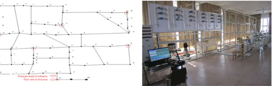
To validate the model built in 3.1 and 3.2, an example pipe network by EPANET model and a physical experimental platform were built to simulate the flow in multi-leak WDNs, as shown in figure1.
Figure 1. The EPANET model with 7 specified leaks marked by red circle (left) and
thephysical pipe network experimental platform (right)
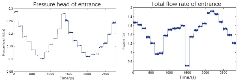
The EPANET model includes15 loops, 62 nodes and 66 pipe segment. It is considered to have 2~ 7 leaks, respectively, thus 6 working conditions of the model are simulated. During the simulation, the real value of the leakage flow rate is simulated by adding an emitter at the specified node, with leakage coefficient α being 0.6 and leakage exponent β being 0.5. Taking the model with 7 leaks for example, the pressure head and the total flow rate are considered as source signals, as shown in figure2.
Figure 2. The pressure head (left)and the total flow rate (right)
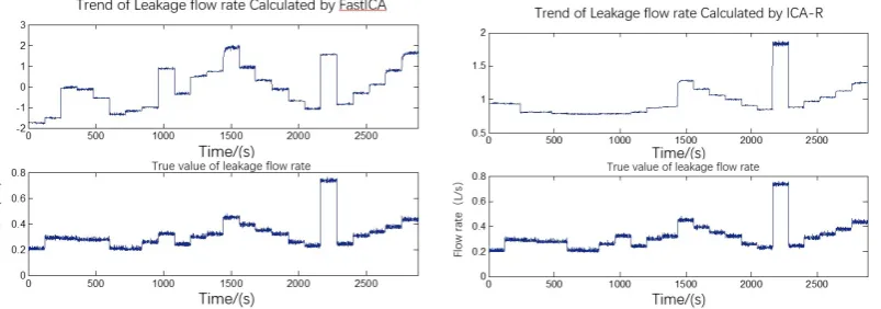
To evaluate the performance of the improved ICA-R algorithm, the trend of actual consumed water flow in time series s (t) and leakage flow rate s (t) are then calculated by both improved ICA-R algorithm and FastICA algorithm [9]. Taking the EPANET model with 7 leaks for example, the leakage discharge trend separated by FastICA and by improved ICA-R algorithm are shown in figure3. The Pearson's correlation coefficient was 16.64% between source signal and leak discharge signal calculated by FastICA, and Pearson's correlation coefficient between ICA-R and source signal is 99.98%. Apparently the separation using improved ICA-R algorithm shows less deviation.
Figure3. Leakage discharge trend separated by FastICA (left) and by improved ICA-R algorithm(right) in EPANET model
The physical pipe network experimental platform consists of 12 loops, 67 nodes and 88 pipe segments. The experimental platform WDN is considered to have 2~6 leaks, thus 5 working conditions of the model are simulated. Taking the model with 6 leaks for example, the pressure head and the total flow rate are considered as source signals, as shown in Figure4.
Figure 4. The pressure head (left)and the total flow rate (right)
at the entrance of physical experimental platform
Table 1. The Pearson's correlation coefficient between source signal and leak discharge signal calculated by FastICA and by ICA-R algorithm in the example EPANET model
Number of leaks Pearson's correlation coefficient by ICA-R
algorithm
Pearson's correlation coefficient by FASTICA algorithm
2 36.37% 76.79%
3 34.93% 92.19%
4 40.73% 95.32%
5 40.73% 90.73%
6 77.47% 94.15%
Taking experimental platform of pipe network with 6 leaks for example, the leakage discharge trend separated by FastICA and by improved ICA-R algorithm are shown in Fig3.Pearson's correlation coefficient was 16.64% between source signal and leak discharge signal calculated by FastICA, and Pearson's correlation coefficient between ICA-R and source signal is 99.98%. Apparently the separation using improved ICA-R algorithm shows less deviation.
Figure5. Leakage discharge trend separated by FastICA (left) and by improved ICA-R algorithm(right) in physical experimental platform
3
Conclusions
EPANET model and the test through physical pipe network experimental platform, it is found that the separation effect of ICA-R is relatively stable, and the Pearson correlation coefficient of the separation signal and the source signal is generally higher than 90%. Even in the face of weak correlated or irrelevant source signals, ICA-R is shown better performance than FastICA. The improved ICA-R algorithm shows high reliability in laboratory testing, field testing is needed for future work.
4
Acknowledgement
The authors gratefully acknowledge the research funding provided by:(1)he National Key Research and Development Program of China: “Prevention and control of public safety risk and emergency technical equipment 2016YFC0802402”, (2) Research and development program of application technology of Harbin: “Research and application of leakage detection and control technology for urban water supply network 2016RAYGJ002”, (3) University and Research Institute of Harbin credit guarantee recommendation project: “Research and application of smart water platform for urban water supply network 2017FF1XJ001”, (4) National Natural Science Foundation of China: “Research on drop-restore pressure leakage mechanism and discretional leakage control of water distribution network. 51778178”, (5) H2020 new project IOT4Win (internet of thing for Water Innovate Network), (6) FP7-ICT-2011-8, WatERP (EC318603) Water Enhanced Resource Planning “Where water supply meets demand.(7)EU Horizon 2020 Research and Innovation program under MSCA-ITN-IoT4Win (765921) Internet of Things for Smart Water Innovative Networks
5
References
[1] M. Farley and S. Trow, "Losses in Water Distribution Networks," Iwa Publishing, 2003.
[2] R. Puust, Z. Kapelan, D. A. Savic, and T. Koppel, "A review of methods for leakage management in pipe networks," Urban Water Journal, vol. 7, pp. 25-45, 2010.
[3] R. Liemberger and M. Farley, "Developing a Non-Revenue Water Reduction Strategy, Part 1: Investigating and Assessing Water Losses," Paper to Iwa Congress, 2004.
[4] M. V. Casillas, V. Puig, L. E. Garzacastañón, and A. Rosich, "Optimal Sensor Placement for Leak Location in Water Distribution Networks Using Genetic Algorithms," in Control and Fault-Tolerant Systems, 2014, pp. 14984-15005. [5] G. Sanz, R. Pérez, Z. Kapelan, and D. Savic, "Leak Detection and Localization through Demand Components Calibration," Journal of Water Resources Planning & Management, vol. 142, pp. 1097-8, 2016.
[6] X. Xie, Q. Zhou, D. Hou, and H. Zhang, "Compressed sensing based optimal sensor placement for leak localization in water distribution networks," Journal of Hydroinformatics, p. jh2017145, 2017.
[7] J. Gao, S. Qi, W. Wu, D. Li, T. Ruan, L. Chen, T. Shi, C. Zheng, and Y. Zhuang, "Study on Leakage Rate in Water Distribution Network Using Fast Independent Component Analysis," in Procedia Engineering. vol. 89, O. Giustolisi, B. Brunone, D. Laucelli, L. Berardi, and A. Campisano, Eds., 2014, pp. 934-941.
[8] J. Mi, "A Novel Algorithm for Independent Component Analysis with Reference and Methods for Its Applications," PLOS ONE, vol. 9, 2014.
[9] Q. Xie, L. Zhang, S. Cheng, S. Hou, L. Peng, and F. Lü, "Application of the FastICA algorithm to PD ultrasonic array signal de-noising," Proceedings of the Csee, vol. 32, pp. 160-166, 2012.