http://www.sciencepublishinggroup.com/j/ajmcm doi: 10.11648/j.ajmcm.20190404.11
ISSN: 2578-8272 (Print); ISSN: 2578-8280 (Online)
Estimation of Parameters in the SIR Epidemic Model Using
Particle Swarm Optimization
Supriadi Putra
*, Khozin Mu'tamar, Zulkarnain
Department of Mathematics, University of Riau, Pekanbaru, Indonesia
Email address:
*
Corresponding author
To cite this article:
Supriadi Putra, Khozin Mu'tamar, Zulkarnain. Estimation of Parameters in the SIR Epidemic Model Using Particle Swarm Optimization. American Journal of Mathematical and Computer Modelling. Vol. 4, No. 4, 2019, pp. 83-93. doi: 10.11648/j.ajmcm.20190404.11 Received: September 30, 2019; Accepted: October 25, 2019; Published: October 30, 2019
Abstract:
Susceptible, Infected and Resistant (SIR) models are used to observe the spread of infection from infected populations into healthy populations. Stability analysis of the model is done using the Routh-Hurwitz criteria, basic reproduction number or the Lyapunov Stability. For stability analysis, parameters value are needed and these values are usually assumed. Given data cannot be used to determine the parameter values of SIR model because analytic solution of system of nonlinear differential equation cannot be determined. In this article, we determine the parameters of the exponential growth model, logistic model and SIR models using the Particle Swarm Optimization (PSO) algorithm. The SIR model is solved numerically using the Euler method based on the parameter values determined by PSO. The simulation results show that the PSO algorithm is good enough in determining the parameters of the three models compared to analytical methods and the Gauss-Newton’s method. Based on the average hypothesis test the relative error obtained from the PSO algorithm to determine the parameters is less than 3% with a significance level of 1%.Keywords:
Growth Mathematical Model, SIR Model, Curve Fitting, PSO Algorithm, Estimation of Parameters1. Introduction
Mathematical models can be interpreted as mathematical equations that explain behavior in the real world. This equation is formed by transforming the form of events in the community into variables or parameters. The mathematical model that is quite widely used is the model in the form of differential equations. For example, the model of motion, whether it is a spring, pendulum or aircraft maneuver, is expressed in a system of ordinary differential equations. In addition, the disease spread model better known as the Susceptible, Infected, Resistant (SIR) model is also expressed in the ordinary differential equation system. The SIR model is very widely used to analyze the spread of diseases in the human environment such as the ebola virus [1], zika [2], malaria [3], diabetes [4]. Not only diseases that attack physically, but diseases that are bad habits can also be analyzed with the SIR model. Mu'tamar [5] developes a SIR model to analyze the spread of habits of consuming alcoholic beverages as well as implemented the optimum control for treatment measures. In addition to the human environment,
the SIR model can also be used to analyze the spread of viruses in a computer environment [6]. If this mathematical model is combined with data, then mathematics can be an excellent tool for environmental observation and the basis for policy making. Unfortunately, to process data and mathematical models in the form of ordinary differential equations is not easy. This is because the process uses the curve fitting which has so far only been carried out on functions that have an explicit form. It is difficult to do in the SIR model because this model cannot be solved analytically so the solution of the equation in the explicit form cannot be determined.
linearization method failed to determine the control of a nonlinear system due to discontinuity. Mu'tamar and Naiborhu [10] use PSO and is combined with fuzzy logic to determine the weighting matrix of the LQR control which is applied to the track control system. Hasni et. al. [11] use PSO to determine parameters in the GreenHouse climate model and compared with genetic algorithms. Jalilvand et. al. [12] use PSO and modify the aspect of random numbers using position and PersonalBest ratios so as to speed up the process of finding a solution. Chiu et. al. [13] applies PSO to determine parameters in the antenna array so that signal noise can be minimized. Solihin and Akmeliawati [14] utilizes PSO to determine the optimum control parameters which are applied to the inverted pendulum linear form.
It should be emphasized here, in other studies that have been done before, the parameters to be determined using PSO are parameters of functions or functions that are explicitly available. The GreenHouse model in [11] uses a mathematical model where explicit solutions are available so that the fitness value can be calculated easily. Whereas in this study, the parameter determined value is the parameter of the mathematical model whose solution is not available using analytical methods. However, the results of determining the parameters of the SIR epidemic model using PSO indicate that the PSO algorithm has succeeded in finding the origin parameters with very low error rates. Based on the average hypothesis test the relative error obtained from the PSO algorithm to determine the parameters is less than 3% with a significance level of 1%.
2. Material and Methods
The method used in this research is the study of literature, which develops previous research. Because the parameter estimation method in dynamic systems has not been done in previous studies, this research will be carried out on a simple model that is an exponential and logistic growth model. Furthermore, the method will be applied to the Susceptible, Infected and Resistant (SIR) epidemic models. The work steps in this research are (1) determining the data to be used as work materials whose characteristics meet the exponential and logistical models, (2) determining the analytical solutions of the exponential and logistical models. Both of these models involve two parameters of unknown value, (3) determining the numerical solution of the logistical model and the SIR epidemic model. The logistic model has again determined its numerical solution for the comparative test of the success of the PSO method in determining parameters, (4) determining the parameter values of each model where the PSO method is used for the whole model, the linear curve fitting method for exponential and logistic models, while the Gauss-Newton’s method only for exponential models, (5) comparing data and function results based on the generated parameter values, (6) specifically for the SIR epidemic model, the data obtained by simulation with predetermined parameter values. Therefore, a hypothesis test is performed to see
whether the resulting parameter gives a small error value compared to the proposed hypothesis value
Furthermore, some definitions and theories related to this research are presented in the following discussion.
2.1. Linear Function Curve Fitting
Lets given n pairs of data ( ,t di i) for i=1, 2,…,n and select the overlay function for that data, f t( )=a0+a t1 with
0, 1
a a ∈R and a1≠0. Defines an error between the data and
the approximation function
2
0 1 0 1
1 1 ( , , ) ( ) 2 n i i i
r a a t a a t d =
=
∑
+ − (1)where di =d t( ).i The goal to be achieved is to minimize the value of r a a t( 0, 1, ) in equation (1) by selecting a a0, 1 that is
appropriate. The values (a a0*, 1*) will minimize equation (1) if satisfy 0 1 0 1 0 1 1 1 ( ) n i i n i i i r
a a t d a
r
a a t d t a = = ∂ = + − ∂ ∂ = + − ∂
∑
∑
(2) with 0 10 and 0,
r r
a a
∂ = ∂ =
∂ ∂ to produce
* *
0 1
1 1
* * 2
0 1 1 1 n n i i i i n n
i i i i
i i
a a t d
a t a t t d
= = = = + = + =
∑
∑
∑
∑
(3)The system of equations (3) can be expressed in a linear system of equations Ax=bwith x ( 0*, 1*)
T a a
= and
1 1 2 1 1 1 A n n i i i n n i i i i t t t = = = = =
∑ ∑
∑ ∑
(4) 1 1 b n i i n i i i d d t = = = ∑
∑
(5)2.2. Particle Swarm Optimization (PSO)
behavior of ant or bee herds developed by Kennedy and Eberhart [7]. The goal function solution is the swarm position calculated by the equation
1 1
xik+ =xik+vik+ (6)
where V is the speed of swarm motion expressed in the equation
1 1 2
vik+ =vki +cγ(Pbik−x )ik +c γ(Gbki −x )ik (7)
The definitions of the symbols in equations (6), (7) are given in Table 1.
Table 1. The Symbols of equation (6) and (7).
Symbol Description
xik Swarm position
vik Swarm velocity
1, 2
c c
Individual and social cognitive swarm, a number that expresses the level of swarm's ability to determine solutions and the ability to develop with the herd. The best value
based on research is c1+c2≤4. [8]
γ Computer generated random numbers
Pb PersonalBest, the best solution of swarm position
Gb GlobalBest, the best solution for all swarms from all
iterations
2.3. The Susceptible, Infected and Resistant (SIR) Epidemic Model
The SIR epidemic model is a mathematical model in the form of a system of ordinary differential equations that is used to describe the spread of disease from infected individuals. The SIR epidemic model is expressed in equations
'( ) ( ) ( ) '( ) ( ) ( ) ( )
'( ) ( )
s t s t i t i t s t i t i t r t i t
α α β β = − = − = (8)
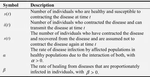
with ( ), ( ), ( )s t i t r t ≥0 and ( )s t +i t( )+r t( )=1 for each time t. The variables and parameters in equation (8) are described in Table 2.
Table 2. The Parameters and variables in equation (8).
Symbol Description
( )
s t Number of individuals who are healthy and susceptible to
contracting the disease at time t
( )
i t Number of individuals who contracted the disease and can
transmit the disease at time t
( ) s t
The number of individuals who have contracted the disease and recovered from the disease and are assumed not to
contract the disease again at time t
α
The rate of disease infection by affected populations in healthy populations due to the interaction of both, with
0.
α >
β The rate of healing from diseases that are proportionately infected in individuals, with β >0.
2.4. Gauss-Newton’s Method
Given system of nonlinear equations, y= f(x).The value xe is the root of the system of nonlinear equation if it satisfies f(x )e =0. To determine the solution of system of nonlinear equations, Gauss-Newton's method can be used, where is given by
1 1
xn+ =xn−J (x ) (x )− n f n (9)
where x is the initial guess and J is the Jacobian matrix of 0 the system of nonlinear equation, i.e
1 1 1
1 2
2 2 2
1 2
1 2
J
n
n
n n n
n
f f f
x x x
f f f
x x x
f f f
x x x
∂ ∂ ∂ ∂ ∂ ∂ ∂ ∂ ∂ ∂ ∂ ∂ = ∂ ∂ ∂ ∂ ∂ ∂ ⋯ ⋯ ⋮ ⋮ ⋱ ⋮ ⋯
2.5. Euler Method for Ordinary Differential Equation Systems
For example, given a first order and autonomous ordinary differential equation system, y '= f t( , y) with initial value
0
y =y(t=0) defined at intervals I∈[0,tf].
The Euler method for solving numerical solutions of systems of ordinary differential equations is given by
1
yn+ =yn+hf t( , y), n=0,1, 2,…,N (10)
where h is the width of partition I which is h tf N
= .
3. Result and Discussion
This section will discuss the determination of parameters contained in the exponential growth model, logistics and SIR epidemic models. The parameter determination method that will be used includes the exact method, the numerical method using Gauss-Newton’s and the PSO algorithm. For the logistics model, parameter determination will be carried out using the exact method and the PSO algorithm. The Gauss-Newton’s method requires a partial derivative of each variable which causes the equations involved in the logistics model to become very complex. In the SIR epidemic model, the parameter determination method used is only the PSO algorithm because there is no analytical method to solve the SIR differential equation system.
3.1. Determination of Exponential Model Parameters
( )
( )
dN t
N t
dt =
λ
(11)where λ is a comparative parameter whose value is positive to describe the increase and negative for the decrease. The analytical solution of an exponential growth model using variable separation is given by
0
( ) t
N t =N eλ (12)
where N0 nitial value, the value of N t( ) when t=t0. To determine the parameters in equation (12), equation (12) needs to be expressed in a linear equation. Transformation of natural logarithms in each of the segments in equation (12) will result.
(
)
( )
0ln N t( ) =λt+ln N (13)
Equation (13) is a linear equation with respect to t with slope λ and intercept ln
( )
N0 . To determine the parameter0
,N
λ from the exponential model of the given data can be done with the following procedure.
Algorithm 1. Determination of exponential model parameters
1. Data input ( ,t di i)
2. Transform data using natural logarithm, called Di. 3. The shape of matrix A is based on equation (4) using
data Di.
4. Form a vector b based on equation (5) using ti and
.
i
D
5. Solve system of linear equations to get parameter values λ, ln
( )
N0 . To obtain N0 can be done usingexponential of ln(N0).
3.2. Determination of Logistics Model Parameters
The logistic growth model is an improvement model of the exponential model by changing the value of proportionality with a linear function with a negative slope. The form of logistic growth model is given by
(
)
( )
( ) ( )
dN t
a bN t N t
dt = − (14)
with a, b is a positive parameter that states the proportion of natural growth and decline due to population saturation. Using the variable separation method, an analytic solution will be obtained from equation (14), i.e.
max ( ) ( ) ln
1 NN t dN t
at c
= + −
(15)
with Nmax =ab is the maximum population. Equation (15) is a linear equation with respect to t with the slope a and intercept c. To determine parameters a, b of the logistic
model from the data provided can be carried out with the following procedure.
Algorithm 2. Determination of logistic model parameters with data
1. Data input ( ,t di i)
2. Set the value Nmaxas the maximum population of di plus a certain positive constant
3. Transform the data using the left column in equation (15), called wi.
4. The shape of matrix A is based on equation (4) using data wi.
5. Form a vector v based on equation (5) using data ti and wi.
6. Solve system of linear equations to get parameter values a c, .
7. The value of parameter b is defined by max a N b= .
3.3. Determines the SIR Model Parameters Using PSO
To determine parameters with PSO, a solution from the SIR epidemic model is needed. Because the SIR epidemic model cannot be solved analytically, this model will be solved numerically, using the Euler method. PSO uses swarm to find food sources, which in computing is the solution to the problem. Because there are
( )
nV parameters in the SIR epidemic model, in this case ,α β with each parameter using nS swarm and updating itM calculations, x is the position matrix of the PSO swarm that stores the solution and is expressed as(
)
x nV×nS itM, (16)
The same is true for V as the velocity matrix for the PSO swarm. Each swarm has its own search history and will store the best search results as PersonalBest. Therefore PersonalBest matrix is defined as the search history of each PSO i.e
(
)
Pb nS×nV itM, (17)
The results of searching for all swarms on one variable will be best selected as a reference for the whole swarm motion step known as GlobalBest. GlobalBest is the best position matrix for all swarms in one parameter throughout the iteration so that it is defined
(
)
Gb nV itM, (18)
Algorithm 3. Determination of SIR epidemic model parameters using PSO
1. Input data ( ,t di i).
7. Set PersonalBest, which is the value of the swarm position in the first iteration
8. Set GlobalBest, the swarm position value that gives the best fitness value.
9. For i = 1: itM
10.Update the swarm position value with equation (6) 11.Update swarm speed values with equation (7)
12.Calculate the ith fitness swarm value using Algorithm 4 13.Determine the PersonalBest of each swarm from first
iteration to ith iteration
14.Determine the entire global swarm from first iteration to ith iteration
15.Check the correctness of one of the following conditions
a) The difference of ith and (i-1)th iteration swarm is less than or equal to tolM
b) The difference in the fitness value of all parameters is less than or equal to the tolM
c) Maximum iteration of itM has been reached 16.If one of the criteria is true, the iteration is stopped 17.End for.
GlobalBest and PersonalBest are determined based on fitness values. Fitness value is the value of the function to determine the solution. The fitness value in the SIR epidemic model is the absolute difference between the data and numerical solutions generated using the Euler method with parameter data from the PSO.
The parameter determination step in the SIR epidemic model using PSO is given in Algorithm 3 and the fitness value is determined by the procedure given in Algorithm 4.
Algorithm 4. Calculation of fitness values using the Euler method
1. Data input ( ,t di i)
2. Input initial values of SIR s i r0, ,0 0.
3. Complete the SIR model in equation (8) with initial values and parameters ,α β for all swarm, t xni, { , }i k for
1, 2, ,
k = … nS using the Euler method in equation (10) 4. Calculate the absolute value of the difference between
the solutions ek =|di−xn{ , }i k | .
5. Sort the value of ekfrom smallest to largest.
3.4. Numerical Simulation
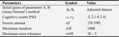
In this section numerical simulations are performed to see a comparison between analytic methods, Gauss-Newton’s and PSO in determining the parameters of dynamic models. For numerical simulation purposes, the basic parameters used in PSO are given in Table 3.
Table 3. The parameters used in numerical simulations.
Parameters Symbol Value
Initial guess of parameters A, B
Gauss-Newton’s method A B0, 0 Adjusted dataset
Cognitive swarm PSO c c1, 2 {1.2,1.8, 2.4}
Swarm amount nS {30,100}
Maximum iteration itM 1000
Maximum error tolerance tolM 1E 5−
First, the exponential model parameters will be determined using analytical methods, Gauss-Newton’s and PSO from temperature and humidity comparison data in the earth's atmosphere [15] presented in Table 4.
Based on the data provided, using the procedure in Algorithm 1 obtained a matrix A and vector b i.e.
80 13 20.32703
A , b
8100 80 693.6217
= =
(19)
Because the determinant of matrix A in equation (19) is not zero then there is a single solution, namely
0
0.0747,N 3.015.
λ= = For PSO three different swarm values will be used with c1=c2 =1.8. Full simulation results are given in Table 5.
Table 4. Humidity based on height.
Temperature (°C) -40 -30 -20 -10 0 5 10 15 20 25 30 35 40
Humidity (g/kg) 0.1 0.3 0.75 2 3.5 5 7 10 14 20 26.5 35 47
Table 5. Results of parameter determination from data Table 4 for the exponentioal model and its error.
No Methods A0 B0 nS itM TOC Ai Bi Error Relative Error
1 Analitik - - - 0.074718 3.015647 25.22 14.736%
2 GN 0.3 0.2 - 100 2.57 4.103670 0.061240 2 1.169%
3 GN 0.5 5 - 100 2.56 0.5 3.75 2.43E+129 142E+127%
4 GN 5 5 - 100 2.57 5 3.75 2.4E+131 142E+129%
5 PSO - - 30 157 3.21 4.103666 0.061235 1.716426 1.003%
6 PSO - - 100 142 2.48 4.103668 0.061235 1.716426 1.003%
7 PSO - - 150 172 3.58 4.103676 0.061235 1.716426 1.003%
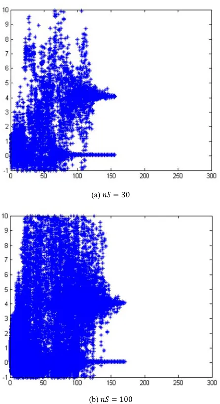
In Table 5 it can be seen that the PSO algorithm generates parameters that make the exponential model approach the data provided compared to the analytic and Gauss-Newton’s methods. In the Gauss-Newton’s method there are different results resulting from the selection of different initial values. The selection of an incorrect initial value in the Gauss-Newton’s method results in a divergent method or does not
succeed in finding a solution. The swarm movement with {30,100}
nS= from the randomly chosen starting point to the final solution point, is given in Figure 1.
will gather at the same point where that point is the final solution which is a parameter of the exponential model.
(a) 30
(b) 100
Figure 1. Swarm movement from initial position to the exponential model parameter point for nS={30,100} from the data in Table 4.
Comparison between data and numerical solutions using parameters determined by PSO and theirs error is given in Figure 2.
(a)
(b)
Figure 2. Numerical solutions of exponential and error models for data in Table 4.
In the logistics model, the method to be compared is the analytical method and PSO. The dataset used is the Bison population data in the Yellowstone area [16] presented in Table 6. Based on the data in Table 6 and using the procedure in Algorithm 2, matrix A and vector b are obtained
57, 495 30 209.276
A , b
110,191, 415 57, 495 40,177.63
= =
(20)
Table 6. Bison population data in the Yellowstone area from 1902-1931.
No Year Population No Year Population No Year Population
1 1902 44 11 1912 192 21 1922 647
2 1903 47 12 1913 215 22 1923 748
3 1904 51 13 1914 229 23 1924 808
4 1905 74 14 1915 270 24 1925 830
5 1906 80 15 1916 348 25 1926 931
6 1907 84 16 1917 397 26 1927 1008
7 1908 95 17 1918 423 27 1928 1057
8 1909 118 18 1919 504 28 1929 1109
9 1910 149 19 1920 501 29 1930 1124
Table 7. The results of the determination of parameters using analytical methods, PSO and their errors.
No Methods nS itM TOC Ai Bi Error Relative Error
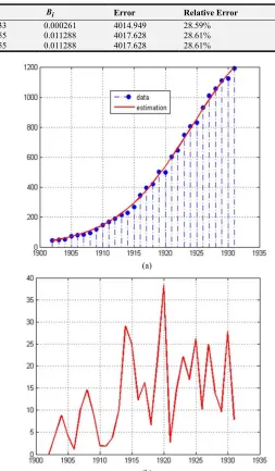
1. Analytic - - - 0.310833 0.000261 4014.949 28.59%
2. PSO 30 226 3.56 17.17955 0.011288 4017.628 28.61%
3. PSO 100 245 7.15 17.17955 0.011288 4017.628 28.61%
Furthermore, the results of the comparison of parameters from the data in Table 6 for the logistic model by comparing the analytical method which is the system of linear equations solution of equation (20) and the PSO algorithm are given in Table 7.
Table 7 shows that the PSO algorithm obtains parameters that make the logistic model approach the data with a very small error rate difference (0.02%) compared to analytical methods. When viewed, the analytical method and the PSO algorithm produce parameter values that are far different but both produce almost the same function values. Swarm movement with
{30,100}
nS= from the randomly selected starting point to the final solution point, is given in Figure 3. The comparison curve between data and numerical solution using parameters determined by PSO and the error is given in Figure 4.
(a) nS=30.
(b) nS=100.
Figure 3. Swarm movement from initial position to the logistical model parameter points for nS={30,100} from the data Table 6.
(a)
(b)
Figure 4. Numerical solutions of the logistic model and its error in the data of Table 4 at t∈[1902,1931].
Table 8. Parameters used to generate data of SIR epidemic model.
No α β No α β No α β No α β
1 0.9756 0.6774 6 0.6136 0.6839 11 0.4152 0.7281 16 0.4459 0.8515
2 0.1614 0.1245 7 0.4105 0.4273 12 0.1491 0.7248 17 0.4971 0.2100
3 0.7945 0.5955 8 0.9692 0.2768 13 0.4943 0.6450 18 0.1561 0.8267
4 0.9244 0.7729 9 0.6532 0.9780 14 0.8487 0.0859 19 0.6979 0.2064
5 0.4663 0.5796 10 0.7714 0.9649 15 0.6778 0.5279 20 0.2047 0.4755
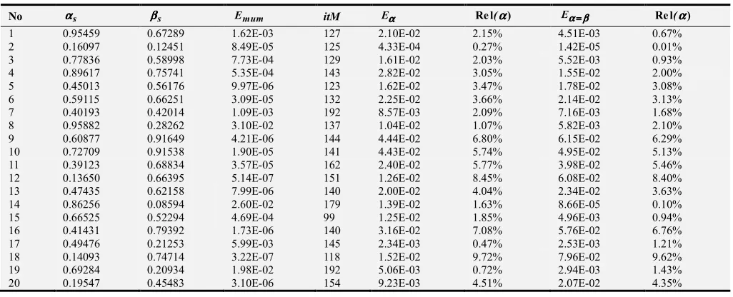
The simulation results of the determination of parameter α and β in Table 8 using PSO are presented in Table 9. Table 9 show Enum that is cumulative absolute error between generated data and numerical solution using the parameters, itM is iteration that PSO needed to obtained desired parameters, Eα and Eβ are absolute errors
parameter α and ,β Rel( )α and Rel( )β are relative errors each parameters. From Table 9, each parameter has error less than 10%. The biggest error occur in parameter set number 18, the smallest error occur at number 2 and average error is 3.35%.
Table 9. The results of the determination of SIR parameters with PSO and its error.
No ααααs ββββs Emum itM Eαααα Re l(αααα) Eα βα βα βα β==== Re l(αααα)
1 0.95459 0.67289 1.62E-03 127 2.10E-02 2.15% 4.51E-03 0.67%
2 0.16097 0.12451 8.49E-05 125 4.33E-04 0.27% 1.42E-05 0.01%
3 0.77836 0.58998 7.73E-04 129 1.61E-02 2.03% 5.52E-03 0.93%
4 0.89617 0.75741 5.35E-04 143 2.82E-02 3.05% 1.55E-02 2.00%
5 0.45013 0.56176 9.97E-06 123 1.62E-02 3.47% 1.78E-02 3.08%
6 0.59115 0.66251 3.09E-05 132 2.25E-02 3.66% 2.14E-02 3.13%
7 0.40193 0.42014 1.09E-03 192 8.57E-03 2.09% 7.16E-03 1.68%
8 0.95882 0.28262 3.10E-02 137 1.04E-02 1.07% 5.82E-03 2.10%
9 0.60877 0.91649 4.21E-06 144 4.44E-02 6.80% 6.15E-02 6.29%
10 0.72709 0.91538 1.90E-05 141 4.43E-02 5.74% 4.95E-02 5.13%
11 0.39123 0.68834 3.57E-05 162 2.40E-02 5.77% 3.98E-02 5.46%
12 0.13650 0.66395 5.14E-07 151 1.26E-02 8.45% 6.08E-02 8.40%
13 0.47435 0.62158 7.99E-06 140 2.00E-02 4.04% 2.34E-02 3.63%
14 0.86256 0.08594 2.60E-02 179 1.39E-02 1.63% 8.66E-05 0.10%
15 0.66525 0.52294 4.69E-04 99 1.25E-02 1.85% 4.96E-03 0.94%
16 0.41431 0.79392 1.73E-06 140 3.16E-02 7.08% 5.76E-02 6.76%
17 0.49476 0.21253 5.99E-03 145 2.34E-03 0.47% 2.53E-03 1.21%
18 0.14093 0.74714 3.22E-07 118 1.52E-02 9.72% 7.96E-02 9.62%
19 0.69284 0.20934 1.98E-02 192 5.06E-03 0.72% 2.94E-03 1.43%
20 0.19547 0.45483 3.10E-06 154 9.23E-03 4.51% 2.07E-02 4.35%
(a) Parameter = 1.
(c) Parameter = 11.
(d) Parameter = 20.
Figure 5. Swarm movement from the initial position to the solution point of the parameters {1, 4, 11, 20} for t∈[0, 30] determined by itM=1000.
(a) Parameter = 1.
(b) Parameter = 4.
(c) Parameter = 11.
(d) Parameter = 20.
Figure 6. The numerical solution of the SIR epidemic model of the parameters {1, 4, 11, 20} for t∈[0, 30] determined by itM=1000.
Figure 5 shows the swarm movement for parameter {1, 4, 11, 20} from the randomly selected starting point to the solution point. The number of swarms used in the simulation of this section is 30 swarm by selecting social and individual
0 5 10 15 20 25 30
0 0.1 0.2 0.3 0.4 0.5 0.6 0.7 0.8 0.9
S(t) I(t) R(t)
0 5 10 15 20 25 30
0 0.1 0.2 0.3 0.4 0.5 0.6 0.7 0.8 0.9
S(t) I(t) R(t)
0 5 10 15 20 25 30
0 0.1 0.2 0.3 0.4 0.5 0.6 0.7 0.8 0.9
S(t) I(t) R(t)
0 5 10 15 20 25 30
0 0.1 0.2 0.3 0.4 0.5 0.6 0.7 0.8 0.9
cognitive at a value of 1.8. It can be seen in Figure 5 that the swarm does not continue to reach itM = 1000 because at a certain iteration point, the stoping condition in Algorithm 3 has been fulfilled. It can be seen in Figure 5 that all swarms gather at two points which are the parameter values to be determined.
(a) Parameter = 1.
(b) Parameter = 4.
(c) Parameter = 11.
(d) Parameter = 20.
Figure 7. Error data and numerical solutions of SIR epidemic models of parameters {1, 4, 11, 20} for t∈[0, 30] determined by itM=1000.
The numerical solution curves of the SIR epidemic model using parameters resulting from the determination using PSO are shown in Figure 6.
The error curve between data and numerical solution from SIR using parameters generated by PSO is shown in Figure 7. The error values are obtained using ex
( )
t = x t( )
−xn( )
t in each time, where xn( )
t is solution obtained from Euler using parameters produced by PSO. Error between data s t( )
and sn( )
t shown in blue line, error between i t( )
and in( )
t shown in red line and error between r t( )
and r tn( )
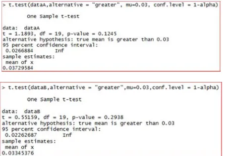
shown in green line. The smallest error is occured at t=0 while the biggest error is occured in around t=5.The final step of this simulation is to test whether the relative error resulting from the α and β parameters generated by PSO is as expected. For this purpose, a statistical hypothesis is made:
0
H : The average relative error of the parameters α, β in Table 9 is less than equal to 3%.
1
H : The average relative error of the parameters α, β in Table 9 is greater than 3%.
Hypothesis testing is done by t-test on R software by selecting a significance level of 1%. The output of the Table 9 test with the t test using R is shown in Figure 8. Figure 8 shows that for a significance level of 1% with a mean of 3% the test yields a p-value = {0.1245, 0.2938} which means it does not reject H0 or in other words, It is true that the relative error produced by PSO to determine the parameters α, β is less than or equal to 3% with a significance level of 1%.
0 5 10 15 20 25 30
0 0.002 0.004 0.006 0.008 0.01 0.012 0.014
eS(t)
eI(t)
eR(t)
0 5 10 15 20 25 30
0 0.002 0.004 0.006 0.008 0.01 0.012
eS(t)
eI(t)
eR(t)
0 5 10 15 20 25 30
0 0.5 1 1.5 2 2.5 3 3.5 4 4.5x 10
-3
eS(t)
eI(t)
eR(t)
0 5 10 15 20 25 30
0 0.5 1 1.5 2 2.5
3x 10
-3
eS(t) e
I(t)
e
Figure 8. The results of the t-test on the parameters of the relative error data in Table 9.
4. Conclusions
This article has discussed the determination of parameters in the exponential, logistical and SIR epidemic models using the PSO algorithm. For each models, the parameter value are obtained by applying an introduced algorithm related to the models. Exponential and logistical models are the basic models from which analytic solutions can be determined. Based on the simulation, it is clear that the PSO algorithm gives better results than the analytical method and the Gauss-Newton’s method. For the SIR model, the data used is simulation data generated from parameters whose values are known. The result of parameter determination using PSO shows that the PSO algorithm can find the origin parameters with a very small error rate. Based on the average hypothesis test, it appears that the relative error resulting from the PSO algorithm for parameter determination is less than 3% with a significance level of 1%. In the simulation of determining SIR parameters, only one PSO parameter is used. This is due to the need for a heavy simulation due to having to solve numerical solutions of the system of differential equations for each swarm in all iterations. For further research, it is necessary to consider the effect of swarm number and cognitive swarm selection on the resulting error. In addition, adaptive PSO can also be applied to studies that have been carried out in terms of swarm convergence speed for the determination of parameters involving SIR and forms of SIR development such as SEIR and SIRS model.
Acknowledgements
This work is supported by University of Riau under DIPA grant 2018. The author is grateful to the referees for their comments and suggestions that helped to improve the paper.
References
[1] Osemwinyen, A. C., Diakhaby, A., Mathematical modelling of the transmission dynamics of Ebola virus, Applied and Computational Mathematics, 4 (4): 313-320, 2015.
[2] Bonyah, E., Okosun, K. O., Mathematical modeling of Zika virus, Asian Pasific Journal of Tropical Disease, 6 (9): 673-679, 2016.
[3] Gebremeskel, A. A., Krogstad, H. E., Mathematical modeling of Endemic Malaria Transmission, American Journal of Applied Mathematics, 3 (2): 36-46, 2015.
[4] Sandhya, Kumar, D., Mathematical model for glucose-insulin regulatory system of diabetes mellitus, Advances in Applied Mathematical Biosciences, Vol 2 No 1, 2011.
[5] Mu'tamar, K., Optimal control strategy for alcoholism model with two infected compartments, IOSR Journal of Mathematics, Vol. 14 Issue 3 Ver. I, 58-67, 2018.
[6] Shukla, J. B., Singh, G., Shukla, P., Tripathi, A., Modeling and analysis of the effects of antivirus software on an infected computer network, Applied Mathematic and Computation, 227 (2014): 11-18, 2014.
[7] Kennedy, J. and Eberhart, R. Particle Swarm Optimization. Proceedings of the IEEE International Conference on Neural Networks, 4, 1942-1948, 1995.
[8] Bratton, D., Kennedy, J., Defining a standard for particle swarm optimization. Proceeding of the 2007 IEEE Swarm Intelligence Symposium, (1-4244-0708-7/07), 2007.
[9] Naiborhu, J., Firman, Mu'tamar, K., Particle swarm optimization in the exact linearization technic for output tracking of non-minimum phase nonlinear systems, Applied Mathematical Sciences, Vol. 7 No 109, 5427-5442, 2013. [10] Mu'tamar, K., Naiborhu, J., Penentuan matriks pembobot pada
kontrol optimal menggunakan adaptive particle swarm optimization, Jurnal Aplikasi Teknologi Universitas Pasir Pengaraian, Vol 8 No 1, 2016.
[11] Hasni, A. Taibi, R., Draoui, B., Boulard, T., Optimization of greenhouse climate model parameters using particle swarm optimization and genetic algorithms, ScienceDirect: Energy Procidia, 6, 371-380, 2011.
[12] Jalilvand, A., Kimiyaghalam, A., Ashouri, A., Kord, H., Optimal tunning of PID controller parameters on a DC motor based on advanced particle swarm optimization algorithm, International Journal on technical and physical problems of Engineering, Vol 3 No 4 Issue 9, 10-17, 2011.
[13] Chiu, C. C., Cheng, Y. T., Chang, C. W., Comparison of particle swarm optimization and genetic algorithm for the path loss reduction in an urban area, Journal of applied science and engineering, Vol 15 No 4, pp. 371-380, 2012.
[14] Solihin, M. I., Akmeliawati, R., Particle swarm optimization for stabilizing controller of self-erecting linear inverted pendulum, International Journal of Electrical and Electronic Systems Research, Vol. 3, 13-23, 2010.
[15] Quantitative Environmental Learning Project at Seattle Central College [Online Data Sets]. Available: https://seattlecentral.edu/qelp/sets/026/026.html.
![Figure 5. Swarm movement from the initial position to the solution point of the parameters {1, 4, 11, 20} for t ∈[0,30] determined by itM =1000](https://thumb-us.123doks.com/thumbv2/123dok_us/976469.1597172/9.595.316.540.75.681/figure-swarm-movement-initial-position-solution-parameters-determined.webp)
![Figure 7. Error data and numerical solutions of SIR epidemic models of parameters {1, 4, 11, 20} for t ∈[0,30] determined by itM =1000](https://thumb-us.123doks.com/thumbv2/123dok_us/976469.1597172/10.595.309.547.79.287/figure-error-numerical-solutions-epidemic-models-parameters-determined.webp)