Research Article
Classification of 7 Arrhythmias from ECG Using Fractal
Dimensions
Kourosh Kiani
*, Farzane Maghsoudi
Department of Electrical and Computer Engineering, Semnan University, Semnan, Iran
*Corresponding Authors:
Kourosh Kiani, Department of Electrical and Computer Engineering, SemnanUniversity, Semnan, Iran, Tel: +989122361274; E-mail: [email protected]
Received: 05 June 2019; Accepted: 21 June 2019; Published: 05 July 2019
Abstract
The statistics indicate a dramatic increase in mortality due to cardiovascular failures in the worldwide. In developing
countries, with lower per capita income, especially in rural areas, late diagnosis of the disease leads to the sudden
death of people. Since electrocardiogram (ECG) is one of the most important tools for diagnosing cardiovascular
diseases, this study has been presented to analyze this highly inexpensive and available signal. Extracted
characteristics of the signal are a good representation of the heart function because of the chaotic, dynamic, and
non-linear behavior of the heart. The fractal dimension is the best representative of the ECG signal which is able to take
into account its hidden complexity. ECG signals are analyzed based on the fractal dimension and Back Propagation
Neural Network (BPN). In this paper, a new technique is introduced for honest classification of 7 arrhythmias from
ECG signals using the fractal dimension. This method is able to identify the exact location of arrhythmias. A
combination of 5 reputable universal databases is used to classify based on the fractal dimension and BPN. The
performance of this method is measured by Sensitivity (SE) and Specificity (SP) indices. According to the results,
the accuracy of this method is equal to 98.83%.
Keywords:
Fractal dimension; Higuchi method; Combined database; ECG; Feature extraction1. Introduction
The statistics indicate that the growing number of deaths is caused by cardiovascular failures. According to the
World Health Organization, about 17.3 million people died of this complication in 2008 [1]. This figure is expected
to reach 23.3 million people by 2030. About 80% of death cases have occurred in countries with low or moderate
per capita income, and most of them have caused by misdiagnosis or late diagnosis of the disease. Since ECG is one
analyzed using this tool [2]. The ECG represents the electrical activity of the heart which includes the regular and
calm contraction of the heart muscles. The ECG waveform analysis is a basis for the diagnosis of different
cardiovascular diseases. The ECG waveform includes 5 major waves of P, Q, R, S, and T [3]. One of the most
important parts of the ECG analysis is the measurement of RR-Interval and ST-segment, which are good
representatives of the variety of heartbeat [4, 5]. Given the non-linear dynamism of the heart and its self-similarity
features, the ECG signals present the fractal properties. As a result, the fractal dimension, which represents the
non-linear dynamism, is an appropriate method for analyzing and extracting the characteristics from these signals [4, 6].
The fractal dimension indicates the ratio of minor variations in the pattern. Moreover, any system that can be
imagined or analyzed geometrically is considered a fractal [7]. Hence, the fractal dimension is used to describe the
fractal objects [7].
Over the last few decades, various techniques have been proposed to solve the ECG classification problems with a
useful diagnosis. In most techniques, features of time [8], frequency [9], time-frequency [10], and non-linear
dynamism [4, 9, 11] have been extracted and then effectively classified. Rai et al. [10] analyzed the ECG signals
based on the neural network and hybrid features (Discrete Wavelet Transforms and morphological). To classify four
types of arrhythmia, George and Mohammad [6] de-noised the signal and calculated the fractal dimension of the
signal using Hurst Power. Sedjelmaci and Reguig [4] extracted the RR-Interval and ST-segment as a feature from
each signal. Then, since the signal information is on regular change, they proposed their own method based on the
regularization dimension analysis of RR-Interval and ST-segment with 4 types of arrhythmia. Martins et al. [11]
used Pan-Tompkins method [12] to extract a QRS complex from the signal. Then, they de-noised the signal by the
wavelet transform. Finally, they classified three types of arrhythmia using Support Vector Machin with an accuracy
of 99%. Mary and Singh [13] used the DFA method to calculate the fractal dimension and detect a normal signal
from an abnormal one. To categorize the natural beat of the ventricle, Mhetre et al. [8] firstly extracted the
morphological features and then classified them using an expert system. Vafaie et al. [14] used a combination of
neural networks and genetic algorithm to detect abnormal conditions of the heart with an accuracy of 98.67%.
After studying the methods, challenges, and shortages, a new method has been proposed in this study for
classification of seven vital types of arrhythmia based on the fractal dimension. To this end, 5 reputable universal
databases have been used. In the procedure of the proposed method, the signal is preprocessed in the first step. After
that, considering the extracted features, the ECG signals are divided into three groups. Then, each signal is classified
based on its own special features. According to the SE and SP indices, the classification accuracy is improved to
98.83%. The contributions of this paper are as follows:
Determine the exact location of the arrhythmia occurrence and its type.
Classification of 7 arrhythmias from ECG signals using the fractal dimension and Back Propagation Neural
Network.
The rest of this paper is organized as the following: Section 2 includes the materials and methods. Section 3 deals
with the fractal dimension used. Section 4 provides experimental results. Finally the paper concludes and the results
are discussed in Section 5.
2. Materials and Methods
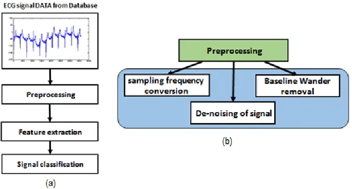
The block diagram of the proposed method has been demonstrated in Figure 1(a). As shown in Figure 1(a), the
entire methodology is divided into three basic steps: preprocessing, feature extraction and classification. The
preprocessing step has been shown in Figure 1(b). Different databases with different sampling frequencies have
been employed in this research. In the preprocessing step, the sampling frequencies have been normalized to a base
frequency that improves the speed of the algorithm and also the accuracy of the classification step. After signal
frequency normalization, de-noising and Baseline wander removal of ECG signals have been done. The second step
of the proposed model is feature extraction. These features must represent the original signal changes. The last step
of the proposed method is dedicated to the classification of arrhythmias. Details of these steps are explained in the
following sub-sections.
Figure 1: (a) Block diagram of proposed method of ECG analysis; (b) Block diagram of Preprocessing.
2.1 Database
Providing a proper database is one of the most important tasks of signal processing. In this research, a combination
of 5 accredited databases from Physionet [15], including 321 annotated files, has been used. This database provides
seven classes of arrhythmias, including Premature Ventricular Complex (PVC), Premature Atrial Contracture
(PAC), Supraventricular Tachycardia (SVTA), Atrial Flutter (A_FLUT), Atrial Fibrillation (A_FIB), Ventricular
Fibrillation (V_FIB) and Normal. These records are extracted from the databases listed below.
European ST-T Database [15],
MIT-BIH Database (Arrhythmia Database, Normal Sinus Rhythm Database, and Supraventricular
QT Database [15],
Creighton University Ventricular Tachyarrhythmia Database [15], Intracardiac Atrial Fibrillation Database [15].
2.2 Preprocessing
Preprocessing is the first step of ECG signal processing. In this step, it is necessary to remove noise from input
signals. Noise removal in the preprocessing of the ECG signal includes different strategies for each noise source
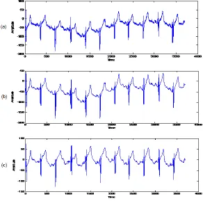
[16]. Preprocessing of ECG signal consists of the sampling frequency normalization, de-noising and baseline
wander removal of ECG signal (Figure 1 (b) and Figure 2). This preprocessing step must have been done before the
feature extraction.
Figure 2: (a) Original or noisy ECG from database; (b) De-noised ECG signal from database; (c) Baseline wander eliminated ECG signal.
2.2.1 Sampling frequency conversion: Due to using the various databases, the first step of preprocessing is to match the frequency of signal sampling. Here, four frequencies, 128, 250, 360, and 1000 Hz, are used. Considering
the mode of the frequencies and the number of the signals at each specific frequency, the frequency equal to 250 Hz
is the base frequency. Sampling frequency conversion is a process which leads to changes in the sampling frequency
in order to obtain a new discrete signal [17]. There are many methods to do this. In this study, Dynamic Time
Warping (DTW) is used for this purpose [18]. Based on this method, the base frequency is selected and then the
next points on the main signal, as shown in Equation 1. In this equation, (x0, y0) and (x1, y1) denote the points before
and after the new sample on the main signal, respectively.
y = y0+ (y1− y0) x−x0
x1−x0 (1)
2.2.2 De-noising the signal: De-noising, which is done before analyzing the electrical activity of the heart, plays an important role in the processing of ECG signals [19]. The frequency band of the ECG signal varies between 0.15 Hz
and 15 Hz. There are many sources of noises in the ECG signal which is placed within its frequency spectrum. In
this step, the structure of different noises, including fluctuations in the heart muscle whose frequency is above 150
Hz, is removed. Since the ECG is non-stable, simple filtering operations will not be effective for de-noising [19].
Because of the proper localization of features in time and frequency domain, DWT methods have been used for this
purpose in the recent studies. In this article, the de-noising method proposed by the authors [20] are used in order to
overcome the problem of DWT variance changes and maintain the physiological characteristics of the signal. In this
algorithm, the signal is divided into 9 levels using the Dual-Tree Complex Wavelet Transform. Threshold values are
calculated using the DF factor and then applied to the first two levels. Thresholding of other levels is done using the
Donoho thresholding method [21]. The threshold of each level is applied to partial coefficients by soft-thresholding.
Then, the signal is reconstructed using modified partial coefficients. Details of the parameters are as the following:
Donoho method λ=√2logM) where M shows the value of coefficients [21]. DF Factor in any sub-band of J is calculated as follows:
DFj= 1
ECEj×
max(djk)
FjSN (2)
Kurtosis =μ4
σ2 (3)
ECEj=
∑ dk jk2
∑ ∑ dj k jk2
×
100 (4)Where, FjSN, µ, and σ2 represent ratio signal kurtosis value in j band to kurtosis value of the signal, mean of partial
coefficients, and variance of partial coefficients. In addition, djk denotes the wavelet coefficients under the band J
[22].
In soft-thresholding, all coefficients are modified or converted into zero with regard to the threshold λ, and a fraction of λ value is considered as the noise value.
di.𝑛𝑒𝑤= {
di− λ di> 𝜆
di+ λ di< 𝜆
0 O. W
(5)
2.2.3 Baseline wander removal: Noise artifacts that affect the ECG signal are called Baseline Wander. Regularly, these noises are in the range of 0.15 to 0.3 Hz and enter the signal using a breathing apparatus. Baseline Wander
removal reduces the heartbeat irregularities in the ECG analysis. There are different ways to remove Baseline
noises by moving the average filter, the signal is smoothed. The results are then plotted in the column vector y. To
smooth the data, a step size of 200 is used to produce better results. After smoothing, the difference between the
smoothed signal and the initial signal are calculated. As a result, the signal obtained is empty of any Baseline
Wander.
2.3 Feature extraction
In this step, extracted features are evaluated based on the fractal dimension. In this study, new and accurate features
are calculated using the fractal dimension. Various methods for the calculation of the fractal dimension, including
Katz, Box Counting, Higuchi, Hurst, Regularization, DFA, Sevcike, and PSD have been investigated that the
Higuchi method can better show the changes and disease in the ECG signal. In addition, this method can examine a
variety of patients more powerfully.
2.3.1 Local-FD and max-ST: After passing the preprocessing stage, a window of 10 seconds is passed over the signal without overlapping. Since this feature indicates different arrhythmias, the detection speed is accelerated
using the window of 10 seconds. Then, the Higuchi dimension is calculated for each window. Finally, the difference
of both consecutive values is calculated. The highest value represents this feature. To calculate the Max-ST, the R
peaks are identified and then the ST-segment value is calculated. This can be done through various methods which
are generally divided into 3 major categories that the first method is the quickest one. In the present study,
Pan-Tompkins method [12] is used. Although this method is more complex than its counterparts, it is one of the most
accurate and widely used methods. The maximum ST-segment value represents Max-ST.
2.3.2 Average-FDH: When the R peaks are identified by Pan-Tompkins method, the fractal dimension in relation to the distance between the two peaks is calculated using Higuchi method. Then, the mean of these values is introduced
as the Average-FDH.
2.3.3 Npac, Npvc and Npsvt: The purpose of these features is to identify peaks that are likely to cause illness. After calculating RR-Interval, the signals with a RR-Interval of greater than 0.2 seconds are diagnosed suspected to
illness. In arrhythmias that occur only in some peaks, there would be a long after any peak of disease. The fractal
dimension related to RR-Interval is calculated using Higuchi method. Since it has been shown that the heart has a
nonlinear system, more severe diseases have a smaller fractal dimension. According to the results, susceptible peaks
can be classified into four groups with regard to the fractal dimension.
Normal: FD >1.56
PAC: 1.37 < FD ≤ 1.56
PVC: 1.3 < FD ≤ 1.37
PSVT: 1 < FD ≤ 1.3
Then, susceptible peaks that are diagnosed normal will be removed. The number of peaks related to each of the
2.4 Signal classification
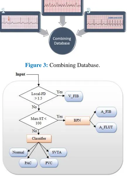
As shown in Figure 3, there are three groups of arrhythmias in this combined database. The first group includes
arrhythmias that occur in some peaks, such as PAC, PVC, and PSVT. The second group involves FLUT and
A-FIB that influence the whole signal. Finally, the third group includes arrhythmias that occur suddenly and continue.
V-FIB is an example of this group in which the heart rate is normal, but suddenly becomes similar to ventricular
fibrillation/flutter. In the proposed algorithm, after the entry of the signal and passing through the previous two
steps, local-FD is firstly calculated and then V-FIB arrhythmia is detected (Figure 4). In V-FIB, the heart signal is
normal at first and then suddenly the rhythm of the heart becomes extremely swirling, as the ECG signal peaks
cannot be detected. Therefore, local-FD is a good benchmark for diagnosing this type of disease which occurs
suddenly and continues. A local-FD of greater than 1.5 is an indication of V-FIB arrhythmia. In the next step, A-FIB
and A-FLUT are separated. These two types of arrhythmia have a sharp rhythm in the whole signal. In addition, the
heart rate is very high. For classification, Max-ST is extracted from the signal. Since the peaks are close to each
other, Max-ST value here is much smaller than the other arrhythmias. As a result, a Max-ST smaller than 100
indicates one of these two arrhythmias. However, if the signal is in this category, A-Fib and A_FLUT arrhythmias
are separated in the second step by using a trained BPN with Average-FDH and Max-ST features. In this step, the
first type of arrhythmias is diagnosed that basically occur as single peaks. Features, including the Average-FDH,
Npac, Npvc, Npsvt, and Max-ST, are extracted from the signal and the disease is diagnosed using Algorithm 1.
Figure 3: Combining Database.
Algorithm 1
If(𝐍𝐩𝐚𝐜 = 𝐍𝐩𝐯𝐜 = 𝐍𝐩𝐬𝐯𝐭 = 𝟎) 𝐎𝐑 (𝐌𝐚𝐱_𝐒𝐓 > 𝟒𝟎𝟎 𝑨𝑵𝑫 𝑵𝒑𝒗𝒄 = 𝟎 𝑨𝑵𝑫 ((𝑵𝒑𝒂𝒄 + 𝑵𝒑𝒗𝒄) ≤ 𝟔)) 𝑶𝑹 ((𝐍𝐩𝐯𝐜 + 𝐍𝐩𝐚𝐜 +
𝐍𝐩𝐬𝐯𝐭) ≤ 𝟏𝟎 𝐀𝐍𝐃 ((𝐍𝐩𝐯𝐜 = 𝐍𝐩𝐚𝐜) ≠ 𝟎 𝐎𝐑 (𝐍𝐩𝐚𝐜 = 𝐍𝐩𝐬𝐯𝐭) ≠ 𝟎 𝐎𝐑 (𝐍𝐩𝐬𝐯𝐭 = 𝐍𝐩𝐯𝐜) ≠ 𝟎)))Then
Signal is Normal.
ElseIf
(𝐌𝐚𝐱_𝐒𝐓 > 𝟒𝟎𝟎) 𝐎𝐑 (𝐍𝐩𝐯𝐜 = 𝐍𝐩𝐚𝐜 = 𝟎) 𝐎𝐑 (𝐀𝐯𝐞𝐫𝐚𝐠𝐞_𝐅𝐃𝐇 ≥ 𝟏. 𝟒𝟑 𝐀𝐍𝐃 (𝐍𝐩𝐯𝐜 − 𝐍𝐩𝐬𝐯𝐭) < 𝟏𝟓) 𝑨𝑵𝑫 (𝑵𝒑𝒔𝒗𝒕 ≠
𝟎 𝑶𝑹 𝑵𝒑𝒂𝒄 ≠ 𝟎)Then
Signal is heart disease Paroxysmal Supraventricular Tachycardia.
ElseIf (𝐍𝐩𝐯𝐜 = 𝐍𝐩𝐬𝐯𝐭 = 𝟎) 𝐎𝐑 (𝐍𝐩𝐚𝐜 > (𝐍𝐩𝐯𝐜 + 𝐍𝐩𝐬𝐯𝐭) 𝐀𝐍𝐃 𝐀𝐯𝐞𝐫𝐚𝐠𝐞_𝐅𝐃𝐇 ≤ 𝟏. 𝟒𝟑)Then
Signal is heart disease Premature Atrial Contracture.
Else
Signal is heart disease Premature Ventricular Contraction.
3. Fractal Dimension
There are different algorithms for calculating the Fractal Dimension, such as Katz [23], box-counting [24], Higuchi
[25], Regularization [26], and etc. Each of them has its own advantages and disadvantages. In this research, these
methods have been studied and reviewed. It has been included that Higuchi is an accurate method and a good
representative of disease. The Higuchi algorithm has the property of intrinsic repeatability as same as the
box-counting method. Assume time series of x={x(1), x(2), …, x(N)}, the Fractal Dimension is calculated as follows.
(i) Construct 𝐾 new time series 𝑥𝑚𝑘 are defined as:
𝑥𝑚𝑘 = {𝑥(𝑚), … , 𝑥(𝑚 + ⌊(𝑁 − 𝑚)/𝑘⌋𝑘)} (6)
Where m=1, 2, …, k shows the initial time value, K denotes the discrete time interval between points.
(ii) Compute the length of each new time series as previously defined:
𝐿𝑚(𝑘) = 1 𝐾⁄ {(𝑁 − 1) ⌊(𝑁 − 𝑚) 𝐾⁄ ⁄ ⌋𝐾∑⌊(𝑁−𝑚)/𝑘⌋𝑖=1 |𝑥(𝑚 + 𝑖𝑘) − 𝑥(𝑚 + (𝑖 − 1)𝑘)|} (7)
Where (𝑁 − 1) ⌊(𝑁 − 𝑚) 𝐾⁄ ⁄ ⌋𝐾is a normalization factor.
(iii) Compute the length of the curve for the time interval K:
𝐿(𝑘) = 1 𝐾⁄ ∑𝑘𝑚=1𝐿𝑚(𝑘) (8)
(iv) Finally, according to the following equation, D represents the Fractal Dimension curve [25].
𝑙𝑜𝑔(𝐿(𝑘)) = 𝐷 𝑙𝑜𝑔(1 𝐾⁄ ) + 𝑏̅ (9)
4. Experimental Results
In this paper, the experiments have been carried out in MATLAB software package 11. The hybrid database consists
of 321 records that have been divided into 7 separate classes: PAC, PVC, SVTA, A_FLUT, A_FIB, V_FIB and
minutes, the shorter amount of time has been considered and analyzed. All features are divided into two groups:
fractal dimension features and morphologic features of ECG signal. While the Max-ST is a morphologic feature, the
Local-FD, Average-FDH, Npac, Npvc and Npsvt are fractal features of the signal. In this research, the signal
classification has been done according to these features by using a BPN with 20 neurons in the hidden layer and a
MLP classifier with 10 neurons in its hidden layer. In order to train mentioned networks, 70% of data is used as the
training data and the remained 30% of data as the test data. The simulation results demonstrate that BPN with 20
neurons in hidden layer achieves the best results (Table 1 and Figure 5). Thus, in this research, a BPN has been used
to classify A_FLUT and A_FIB using Average-FDH and MAX_ST.
Figure 5: performance chart of BPN.
Accuracy (%) Number of correct classification
Number of neurons in
hidden layer Methods Testing Data Training Data Testing Data Training Data 100 95 10 21 10 BPN 100 100 10 22 20 90 95 9 21 10 MLP 90 100 9 22 20 SP (%) SE (%)
Number of correct classification
Total A_FIB A_FLUT 94 100 31 16 15 10 BPN 100 100 32 16 16 20 87 100 30 16 14 10 MLP 100 94 31 15 16 20
The performance of the classifier has been evaluated by using the most familiar metrics: SE and SP [27].
𝑆𝐸(%) = 𝑇𝑃 (𝑇𝑃 + 𝐹𝑁)⁄ × 100 (10)
𝑆𝑃(%) = 𝑇𝑁 (𝑇𝑁 + 𝐹𝑃)⁄ × 100 (11)
Where TP is the number of true positive samples, TN is the number of true negative samples, and FN is the number
of positive samples. The most important metric for evaluating the overall system performance is usually accuracy
[27]:
𝐴𝑐𝑐𝑢𝑟𝑎𝑐𝑦(%) =𝐶𝑜𝑟𝑟𝑒𝑐𝑡𝑙𝑦 𝑐𝑙𝑎𝑠𝑠𝑖𝑓𝑖𝑒𝑑 𝑠𝑎𝑚𝑝𝑙𝑒𝑠
𝑇𝑜𝑡𝑎𝑙 𝑛𝑢𝑚𝑏𝑒𝑟 𝑜𝑓 𝑠𝑎𝑚𝑝𝑙𝑒𝑠 (12)
Accuracy 98.83%
SE 99.74%
SP 96.84%
Table 2: The results of classification using the proposed algorithm.
SE and SP Normal PVC PSVT PAC A_FIB AF V_FIB
SE 99.1 100 99.1 100 100 100 100
SP 100 100 97.9 80 100 100 100
Table 3: The comparison between SE and SP from each class according to the proposed algorithm.
Table 2 shows the results of classification using those features which have been extracted based on the fractal
dimension. This classification of 7 classes has been achieved the precision of 98.83%. Table 3, shows the calculation
of SE and SP for each class in comparison to each other. PVC, A_FLUT, A_FIB and V_FIB have been completely
separated with SE=100 and SP=100; so, fractal dimension is an appropriate representative of them. SE and SP for
the Normal class are 99.1 and 100, respectively. Thus, it has been separated perfectly as well; however, in some
cases, other arrhythmias have been incorrectly detected as Normal. SE=100 and SP=80 for PSVT class demonstrate
that sometimes the disease associated with PSVT class is diagnosed incorrectly. Finally, SE and SP for PAC class
are 99.1 and 97.9, respectively. It shows that the proposed algorithm is less sensitive at the boundary of this disease.
Therefore, the proposed algorithm has some sensitivity at the boundary of diagnosis of Normal and PAC diseases
and also at the boundary of diagnosis of PAC and PSVT diseases.
5. Discussion and Conclusion
The main objective of this study was to classify a variety of hazardous arrhythmias with high accuracy based on a
wide variety of disease-rich databases. In most studies, a maximum of four arrhythmias is classified with a limited
sufficient number of files. In this paper, a new method based on the fractal dimension of the ECG signal was
proposed which is the best representative of the electrical activity of the heart, with regard to the chaotic system of
the heart. The fractal dimension is able to examine minor changes in complex signals. The proposed algorithm is
able to determine the exact location of the arrhythmia occurrence and its type. In the proposed method, the signal
was preprocessed in three steps and the features were extracted based on the fractal dimension and morphological
characteristics of the signal. Then, classification was done based on extracted features. The performance of this
method was measured by SE and SP indices. According to the results, the accuracy of this method was equal to
98.83%. Increasing the accuracy and the number of arrhythmias under study can be good recommendations for
future studies.
Conflict of Interest
The authors claim that they do not have conflict of interest.
Acknowledgment
During this study, we also would like to demonstrate our appreciation to the physio bank for sharing databases of
heart disease and biometric signals.
References
1. Mendis S, Puska P, Norrving B. World Health Organization. Global atlas on cardiovascular disease
prevention and control. Geneva: World Health Organization (2011).
2. Kirk KJ, O’Shea J, Ruhf LK. ECG interpretation made incredibly easy!. Chris Burghardt. 5 (2011).
3. Maglaveras N, Stamkopoulos T, Diamantaras K, et al. ECG pattern recognition and classification using
non-linear transformations and neural networks: A review. International journal of medical informatics 1-3
(1998): 191-208.
4. Sedielmaci I, Reguig FB. Detection of some heart diseases using fractal dimension and chaos theory. In
2013 8th International Workshop on Systems, Signal Processing and their Applications (WoSSPA) 1
(2013): 89-94.
5. Castiglioni P, Faini A, Lombardi C, et al. Characterization of apnea events in sleep breathing disorder by
local assessment of the fractal dimension of heart rate. In2014 8th Conference of the European Study
Group on Cardiovascular Oscillations (ESGCO) 8 (2014): 107-108.
6. Oweis R, Hijazi L. A computer-aided ECG diagnostic tool. Computer methods and programs in
biomedicine 3 (2006): 279-284.
7. George JJ, Mohammed EM. Heart disease diagnostic graphical user interface using fractal dimension. In
2013 International Conference on Computing, Electrical and Electronic Engineering (ICCEEE). 1 (2013):
8. Pipberger HV, Arms RJ, Stallmann FW. Automatic Screening of Normal and Abnormal
Electrocardiograms by Means of a Digital Electronic Computer. Proceedings of the Society for
Experimental Biology and Medicine 1 (1961): 130-132.
9. Addison P. Fractals and Chaos. Napier University, Edinburgh (1997).
10. Mhetre MR, Vaishampayan A, Raskar M. ECG Processing & Arrhythmia Detection: An Attempt.
International Journal of Engineering and Innovative Technology (IJEIT) 2 (2013): 272-276.
11. Ebrahimzadeh E, Pooyan M, Bijar A. A novel approach to predict sudden cardiac death (SCD) using
nonlinear and time-frequency analyses from HRV signals 2 (2014): e81896.
12. Rai HM, Trivedi A, Shukla S. ECG signal processing for abnormalities detection using multi-resolution
wavelet transform and Artificial Neural Network classifier. Measurement 9 (2013): 3238-3246.
13. Martis RJ, Acharya UR, Min LC. ECG beat classification using PCA, LDA, ICA and discrete wavelet
transform. Biomedical Signal Processing and Control 5 (2013): 437-448.
14. Spasić S, Savic A, Nikolic L, et al. Applications of Higuchi’s fractal dimension in the Analysis of
Biological Signals. In2012 20th Telecommunications Forum (TElFOR) 1 (2012): 639-641.
15. Pan J, Tompkins W. A real-time QRS detection algorithm. IEEE Transaction on biomedical Engineering 3
(1985): 230-236.
16. Mary HM, Singh D. Fractal dimension of electrocardiogram: distinguishing healthy and heart-failure
patients. Journal of Electrocardiology 1 (2013): e21-e37.
17. Vafaie MH, Ataei M, Koofigar HR. Heart diseases prediction based on ECG signals’ classification using
agenetic-fuzzy system and dynamical model of ECG signals. Biomedical Signal Processing and Control 1
(2014): 291-296.
18. Kumar G, Kumaraswamy YS. Spline activated neural network for classifying cardiac arrhythmia 8 (2014):
1582-1590.
19. Physiobank archive index.
20. Rai HM, Trivedi A. De-noising of ECG waveforms using multiresolution wavelet transform. International
Journal of Computer Application 18 (2012): 25-30.
21. Oppenheim AV, Schafer RW. Discrete-Time Signal Processing 3 (2011): 1120.
22. Rabiner LR, Schafer RW. Introduction to Digital Speech Processing. Inc, Hanover (2007): 200.
23. Kania M, Fereniec M, Maniewski R. Wavelet denoising for multi-lead high resolution ECG signals.
Measurement science review 4 (2007): 30-33.
24. Raj VN, Venkateswarlu T. ECG signal denoising using undecimated wavelet transform. In2011 3rd
International Conference on Electronics Computer Technology 1 (2011): 94-98.
25. Maghsoudi F, Kiani K. A powerful novel method for ECG signal de-noising using different thresholding
and Dual Tree Complex Wavelet Transform. the 2th Int. Knowledge-Based Engineering and Innovation
(2015).
26. Donoho DL, Johnstone IM. Adapting to unknown smoothness via wavelet shrinkage. Journal of the
27. Sharma LN, Dandapat S, Mahanta A. ECG signal denoising using higher order statistics in Wavelet
subbands. Biomedical Signal Processing and Control 1 (2010): 214-222.
This article is an open access article distributed under the terms and conditions of the
Creative Commons Attribution (CC-BY) license 4.0