Efficient power component identification with long short-term memory and deep neural network

network

Jingsheng Lei

, Wenbin Shi

, Zhichao Lei

and Fengyong Li

Abstract

This paper tackles a recent challenge in patrol image processing on how to improve the identification accuracy for power component, especially for the scenarios including many interference objects. Our proposed method can fully use the patrol image information from live work, and it is thus different from traditional power component

identification methods. Firstly, we use long short-term memory networks to synthesize the context information in a convolutional neural network. Then, we constructed the Mask LSTM-CNN model by combining the existing Mask R-CNN method and the context information. Further, by extracting the specific features belonging to the power components, we design an optimization algorithm to optimize the parameters of Mask LSTM-CNN model. Our solution is competitive in the sense that the power component is still identified accurately even if the patrol images contain much interference information. Extensive experiments show that the proposed scheme can improve the accuracy of component recognition and has an excellent anti-interference ability. Comparing with the existing R-FCN model and Faster R-CNN model, the proposed method demonstrates a significantly superior detection performance, and the average recognition accuracy is improved from 8 to 11%.

Keywords: Power component identification, Long short-term memory, Convolutional neural network, Anti-interference, Live work inspection

1 Introduction

With the rapid development of artificial intelligence, live working robots that can perform automatic inspection have received extensive attention from major power grid corporations [1]. For power systems, blackouts mean a drop in economic efficiency [3]. To maintain a good oper-ating condition of the equipment, machine vision is added in a live working robot to obtain more information about the environment [4] and provide the ability of non-contact measurements. This ability does not pose any danger to workers and thus improve the safety of the system [2]. Also, machine vision is also able to replace the long-term work of the human eye so that the continuous monitoring and identification can be achieved successfully.

*Correspondence:[email protected]

1_{College of Computer Science and Technology, Shanghai University of Electric}

Power, Shanghai, 200090 People’s Republic of China

3_{College of Automation Engineering, Shanghai University of Electric Power,}

Shanghai, 200090 People’s Republic of China

Full list of author information is available at the end of the article

Different from the traditional identification of power components [5], the images from live working robots have complex backgrounds, high density of parts, and high timeliness requirements and contain many interfer-ence objects. In this sense, traditional power component identification cannot be applied well to the patrol images from live working robots because they mainly use manu-ally designed features and segmentation algorithm, where classical features include SIFT (scale-invariant feature transform) [6], edge detector [7], and HOG (histogram of oriented gradients) [8], while the segmentation algorithms are mainly based on peripheral contour skeleton [9] and adaptive threshold [10]. However, applying these methods to automatic detection is not practical due to the following drawbacks: (1) they are often based on specific categories in the design principle so that their accuracy is lower and the scalability is not stronger. and (2) these methods always have a loose structure and lack comprehensive uti-lization of low-level features to achieve the goal of optimal global identification.

Compared with the traditional method, Ren et al. proposed a new approach, named by Faster-RCNN (faster region-based convolutional neural network) [11]. Regarding structure, Faster-RCNN has integrated feature extraction, proposal extraction, bounding box regression (rectangular refine), and classification into a network. It leads to a significant improvement in overall performance and detection speed. R-FCN is another target detec-tion structure proposed by [12]. It modified the previous Faster-RCNN structure by moving the convolutions to the front of the ROI layer. R-FCN used a position-sensitive feature map to evaluate the probability of each category and was thus more accurate in positioning. Although the detection rate was improved, R-FCN cannot recognize the specific contour of the target. Due to this drawback, R-FCN has a limited range of application. Mask R-CNN was proposed by K. He [13], a researcher of Facebook AI, in 2017. This method expands the object detection tech-nology and achieves pixel-level segmentation and contour segmentation of targets by using bilinear interpolation. Law method, proposed by [14], reduced the loss of space symmetry and has better recognition effect in scenes with a transparent background and foreground segmentation. However, it does not have sufficient adaptability to power component scenes with many interference factors and cannot fully exploit the image’s associated information.

To improve the identification precision for power com-ponent, this paper proposes an efficient power component identification with long short-term memory and deep neural network. Based on Mask R-CNN, we design Mask LSTM-CNN model to integrate context features in the classification and regression layers through LSTM neu-ral network [15]. Firstly, we use long short-term memory networks to synthesize the context information in a con-volutional neural network. Then, we constructed Mask LSTM-CNN model by combining the existing Mask R-CNN method and the context information. Further, by extracting the specific features belonging to the power components, we design an optimization algorithm to opti-mize the parameters of Mask LSTM-CNN model [16]. Extensive experiments show that the proposed scheme has an excellent anti-interference ability and verify that the power component is still identified accurately even if the patrol images contain much interference information. Comparing with the existing R-FCN model and Faster R-CNN model, the detection accuracy of proposed scheme has a significant improvement with a range from 8 to 11%.

The rest of this paper is organized as follows. Section2 presents several traditional power component identifica-tion schemes. In Secidentifica-tion3, we provide the details of the proposed approach and introduce the designing proce-dure of Mask LSTM-CNN. Subsequently, comprehensive experiments are performed to evaluate the performance

of the proposed scheme. The experimental results and corresponding discussions are presented in Section 4, respectively. Finally, Section5concludes the paper.

2 Related works

2.1 Power station identification based on Faster-RCNN method

Following R-CNN [17] and Fast R-CNN [18], Faster-RCNN was proposed by [11]. This method can identify region proposals by using a regional proposal network (RPN), which replaces previous methods such as Selective Search [19] and Edge Boxes [20]. RPN and the detection network share the convolutional characteristics of the whole map so that detection for a region can take less time [21]. The structure of the Faster-RCNN neural network is shown in Fig.1.

RPN is a full convolutional-based network [22], and it can simultaneously predict the position of the target pic-ture area and the target score (the probability value of the real target) of the input picture. Meanwhile, RPN is also an end-to-end network training method to generate high-quality regional proposal boxes for Fast R-CNN clas-sification detection. With an optimization method, RPN and Fast R-CNN can share convolution features during training. Combing these two models, an overall structure, named by “RPN+Fast R-CNN,” is integrated. In this struc-ture, RPN network is mainly used to generate high-quality proposal area boxes, while Fast R-CNN is used to learn high-quality proposed area features and classification.

Faster R-CNN designs the network RPN to extract candidate areas and replaces the selective search with

Fig. 2The structure of R-FCN

lower efficiency. This process significantly improves the detection speed of the entire model. However, it can only determine the target’s general location instead of the spe-cific power component’s position. Overall, this model has a low recognition rate when the power components are occluded. Thus, it cannot meet the on-site requirements for power component identification.

2.2 Power station identification based on R-FCN method

The target detection of the regional-based full convolu-tional network [22] is divided into two steps: position-ing a target and then classifyposition-ing the target to a specific category. First, R-FCN model uses a rudimentary con-volutional network to generate a feature map. Then, the regional feature map is used to generate the feature map before and after the full map is constructed. The model determines the target’s outline by searching and filtering [23] scene images through these feature maps. Finally, the classification framework recognizes the target.

Figure2 demonstrates the structure of R-FCN model.

The target image is passed through a basic convolutional network to generate feature maps and input these feature maps into a full-volume network to generate a score bank of position-sensitive score maps. The results of the basic convolutional network go through the RPN network to generate RoI. For a RoI of sizew×h(obtained by the RPN network), the target frame is divided into k× k subar-eas, each subarea is of sizew×h/k2. For anyone subarea bini,j, j ≤ k −1, define a location-sensitive pooling operation:

rc(i,j|∇)=

(x,y)∈bin(i,j) 1

nzi,j,c(x+x0,y+y0|∇) (1)

whererc(i,j|∇)is the pooled response of subarea bin(i,j)

to c categories and zi,j,c stands for a location-sensitive

score map corresponding to subarea bin(i,j). x0 + y0

represents the coordinates of the upper left corner of the target candidate box, n is the number of pixels in subarea bin(i,j), and∇ represents all the learned param-eters of the network. The model calculates the average

of pooled response output rc(i,j|∇) for k × k

sub-regions and uses the softmax regression classification method to obtain the probability that it belongs to each category.

R-FCN integrates the target’s position information into ROI pooling by position-sensitive score map, which solves the problem that the ROI pooling of Faster-RCNN net-work has no translation invariance. Thus, this model improves the accuracy of target detection and classifi-cation so that the operating efficiency of the model is significantly superior. However, it is evident that the R-FCN model still cannot detect the specific location of the target and lacks the robustness to the scene of power components with many interfering objects.

3 Recognition of power components based on Mask LSTM-CNN

Although the Faster-RCNN and R-FCN methods improve the processing speed and accuracy of part identification models, they cannot refine the specific contours of power components so that live working robots cannot accurately identify components’ orientations through such methods.

Fig. 4The schematic diagram of RPN

Moreover, the recognition rate of above two methods will obtain an inferior performance and cannot meet the com-plex industrial environment if power components suffer some. In this section, we combine Mask-RCNN to con-struct an efficient Mask LSTM-CNN model to sufficiently reduce the influence of obstructions on the recognition of targets.

3.1 Neural network model for power component identification

Proposed Mask LSTM-CNN model consists of four parts: pre-training CNN model, RPN network, RoI-Align layer, and detection network layer and Mask layer. The specific

structure of the model is shown in Fig. 3. The model

uses LSTM to correlate ROI information before the tar-get is identified to reduce the effect of obstacles on the power component. The model improves the accuracy of power component recognition by learning the dependen-cies between regions.

(1)Pre-training CNN model

Inspired by the existing CNN model, we use ResNet (a further comparison during the experiment) to pre-train the data in the coco2017 image classification task. The data collected from the collected power compo-nent inspection data is used to improve and eventually build a complete CNN model. The CNN model is the basis of the proposed method, and it provides the fea-ture map required for subsequent RPN networks and detection networks [24]. The feature map contains fea-tures from the deep convolution of the input image, and Euclidean distances between features of objects are pro-portional to the differences between those objects. That is to say that the feature map can differentiate objects well [25].

(2)RPN network

The power component image generates a multi-channel feature map through the previous CNN network. The RPN network applies a sliding window to these feature maps and uses the anchor mechanism to determine and classify the target region of the feature map. Finally, the back-propagation algorithm is used to tune the regional proposal network.

A plurality of convolution kernels in the output layer is used to perform a convolution operation, and then, a three-dimensional tensor is obtained. The tensor is used as the input of two independent convolution layers to con-vert the information in the feature map into the position information of the candidate region and the probability information of the context. As shown in Fig.4, the red area in the figure is the search area. In the picture, only part of the search target box is drawn.

Fig. 6The structure of detection and Mask layer

RPN uses nine search boxes to search for an area with aspect ratios of 1:1, 1:2, and 2:1. The RPN network can get approximate 20,000 search boxes from an original input image. In practical applications, some search boxes beyond the border of the image are removed. Mean-while, NMS (non-maximal suppression) [26] method is used to handle the overlapping of search boxes on the same target. The above strategies can signifi-cantly improve the search efficiency of candidate target boxes.

RPN completes the search of candidate areas on the output layer of the rudimentary convolutional network and provides candidate areas for the subsequent target detection network, which improves the efficiency of the entire model.

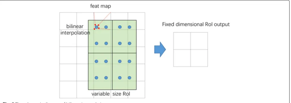
(3)RoI-Align layer

RoI-Align optimizes the problem of pixel bias and uses bilinear interpolation to obtain the image values at the pixels whose coordinates are floating-point num-bers. Finally, the entire feature aggregation process is integrated into continuous operation. ROI-Align layer traverses each candidate areas and keeps floating-point

boundaries unquantified. Thexn, it divides the candi-date area into k ×k units and holds the boundaries of each unit unquantified. Inside each unit, the fixed four coordinate positions are calculated by bilinear interpo-lation. The interpolation method calculates the values of these four locations and then performs the maxi-mum pooling operation. The specific process is shown in Fig.5.

In the back-propagation of the RoI-Align layer,xi×(r,j)

is the coordinate position of a floating point (sample point calculated during forwarding propagation). In the feature map before pooling,each point within the window that has size two by two and centers atxi ×(r,j) should receive

the gradient w.r.t the corresponding point yrj gradient,

the back-propagation formula of the RoI-Align layer is as follows:

∂L ∂xi =

r

j

d(i,i×(r,j))<1(1−k) (1−w) ∂l ∂yrj

(2)

Fig. 8Illustrations in the sample:a“original image” andb“training sample”

where d represents the distance between two points,

andk andw describe the difference betweenxi, the

longitudinal coordinate, and xi ∗ (r,j), the transverse

coordinates. Here, the bilinear interpolation coefficient is multiplied by the original gradient.

The RoI-Align layer solves the problem of RoI misalign-ment between the feature map and the original image, and it obtains better measurement results through more rig-orous positioning metrics, which relatively improves the accuracy of the mask.

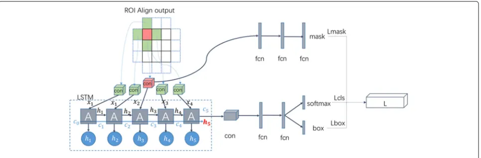
(4)Detect network layer and Mask layer

The result of the regional proposal generated accord-ing to step (3) is the input of the detection network and the Mask layer, wherein the detection network is composed of a classification network and a regional location network. The specific structure is shown in Fig.6.

The detection network uses the convolutional network to pre-convolve each ROI and its top, bottom, left, and right regions to extract the high-dimensional feature vec-tor as the input to lstm [27][28]. The connection status

of the memory unit and various doors are shown in the blue area in Fig. 6. In the figure, xt denotes the

input of different regions, andhtdenotes the output oft

region. The sigmoid function transforms the input infor-mation by multiplying point by point. Forget gate deter-mines whether to save the previous area from the stored state-ht. The input gate determines the information that

needs to be updated. The entire unit updates the storage status through forget and input gatesct. The output gate

[29] determines whether to store information in the mem-ory for output. Through five inputs xt and each hidden

outputht, the final output ish5. The concrete structure

of hidden layer A is shown in Fig.7. When thetth block region of the sequence enters the network, the input of the LSTM hidden layer includes the current input xt of

the network, the hidden layer output vectorxt−1 at the

previous time, and the hidden layer statect−1. The task

of the hidden layer is to calculate and output the vector

htand update the state to obtainct. For this hidden layer,

the oblivion gateft, the input gate, and the outputotgate

are added. Oblivion gateftdetermines which information

Fig. 10Three classification results based on disturbed samples

in statectis discarded. Input gateitdetermines which of

the updated information fromxtandht−1 can be used

for statusct updates. After oblivion gate and the output

gate, statectupdate is completed. The purpose of adding

the hidden layer state in the LSTM is to make it affect the outputhtof the hidden layer, so the output gateotis used

to determine how the statect affects the calculation of

theht.

The sigmoid activation function is shown inδin Fig.7. The calculation expressions of the three new additions, the hidden layer outputht, and status updatectare

calcu-lated as follows:

ft=δ

W_f ·[xt,ht−1]+bf

(3)

it=δ (Wi·[xt,ht−1]+bi) (4)

ot=δ (Wo·[xt,ht−1]+bo) (5)

ct=tanh(Wc·[xt,ht−1]+bc)+ft·ct−1 (6)

ht=ot·tanh(ct) (7)

The last output connects two layers of full-connected

out-put k + 1-dimensional array p and 4× k-dimensional

arrayt, and arrayprepresents the probability of belonging

to classk and background. Output a discrete probability distribution for each RoI (Region of Interesting):

p=(p0,p1· · ·,pk) (8)

p is computed using softmax from the k +1 full

con-nection layer. The array t represents the parameters

that should be pan-scaled when belonging to thek-type respectively:

tk =

t_xk,t_yk,t_wk,tk_h

(9)

kdenotes the index of the category,tk_xandt_ykare the trans-lations invariant w.r.t the scale of the object proposal,tk

w

andt_hk are the height and width of the object relative to the object proposal in space. The probability correspond-ing to the real classificationudetermines the value of loss functionLclsof the classification layer:

Lcls(p,u)= −logpu (10)

The loss functionLboxof box frame detection is obtained

by comparing the difference between the prediction pan-ning scaling parameter tu and the real panning scaling

parameterv, which corresponds to the actual classifica-tion. The specific formula is as follows:

v=(vx,vy,vw,vh) (11)

Lbox(tu,v)= 4

i=1

smoothL1

tu_i −vi (12)

Among them, smoothL1 loss function:

smoothL1(X)=

0.5x2(if|x|<1)

|x| −0.5(otherwise) (13)

The last layer of the full convolutional layer is predicted from the probability that the candidate region box belongs to each category, the score, and the more appropriate loca-tion of the target object’s outer frame, which uses four parameters relative to the two region translation and two scaling of the candidate region frame [30].

The Mask layer has an output ofk×m2_{dimensions for}

each RoI,K (class number) binary mask with resolution

m×m. Therefore, the author uses a per-pixel sigmoid and definesLmaskas the average binary cross-entropy loss. For

a RoI belonging to thekth category,Lmask only considers

thekth mask (other mask inputs do not contribute to the loss function). Such a definition would allow the algorithm to generate a mask for each category, and there would be no inter-class competition. Mask layer loss function:

Lmask(Cls_k)=Sigmoid(Cls_k) (14)

The total loss function can be represented as the sum of the loss functions w.r.t classification error, detection error, and segmentation error.

L=Lcls+Lbox+Lmask (15)

Finally, the network is fine-tuned using the back-propagation algorithmthrough pre-marked information [31].

3.2 Detection and identification process

As can be seen from the above process, the two networks can eventually share the same characteristic information, which improves the information utilization rate. The RoI-Align layer reduces the loss of spatial symmetry and cor-relating the knowledge of the upper and lower regions of the ROI enhances the robustness of the model. The Mask layer can achieve pixel-level segmentation.

The process of detection and identification is as follows:

Step 1: A series of convolution operations are per-formed on the entire image to obtain a feature map.

Step 2:Generate a large number of candidate areas on the feature map by the regional proposal network.

Step 3:Non-maximum suppression of candidate region boxes, retaining the first few boxes with higher scores.

Step 4: Take out the feature in the candidate region frame on the feature map to form a high-dimensional fea-ture vector. Calculate category scores from the detection

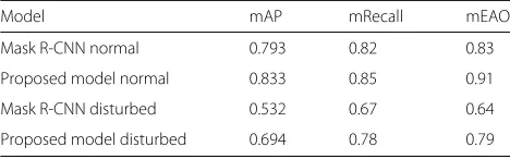
Table 1Comparison of two models mAP, recall, and mEAO

Model mAP mRecall mEAO

Mask R-CNN normal 0.793 0.82 0.83

Proposed model normal 0.833 0.85 0.91

Mask R-CNN disturbed 0.532 0.67 0.64

Proposed model disturbed 0.694 0.78 0.79

network and predict more appropriate target peripheral frame positions.

Step 5:The corresponding binary mask is predicted for each feature map according to the classification in (4).

The method shows through experiments that under the identification of power components with obstructions, solved the problem when the recognition rate is low.

4 Results and discussion

In this section, we validate the proposed scheme by some images from a real power station. Live working robot captures images with high resolution, including rapid zooming of the target size. The angle of the captured image is diverse and random. Three types of power com-ponents are considered: transformers, isolation switches, and circuit breakers.

4.1 Training sample processing

The dataset comes from the substation inspection image. The original image size is 1200 × 900 (Fig.8)a, and we intercept the square block image with the target as the main body and uniformly reduce it to 800×600 (Fig.8)b as a training sample.

4.2 Training sets and test sets

In this test, for each type of component of transformers, isolation switches, and circuit breakers, 1200 training samples were used. A total of 3600 samples constitute a training set; 400 test images of each type and a total of 1200 images constitute a test set. The outer box is marked for the power components in each picture in the training set. For the test set, all the electric components appearing in each picture are marked.

Table 2Comparison of models mAP based on different basic CNN

Faster-RCNN R-FCN Proposed model

VGG-19 0.763 0.791 0.813

ResNet-50 0.781 0.797 0.831

ResNet-101 0.789 0.817 0.846

ResNeXt-50 0.791 0.821 0.845

During the test, it is considered as an auspicious recog-nition when the overlapped area of the identified outer frame and marked outer frame reaches more than 80% of the marked outer frame. In this experiment, average pre-cision, recall rate, and effective area occupancy rate are used to judge the accuracy of identification. Among them, the AP (average precision) is as follows:

AP= ncP

ncA

(16)

wherencPindicates the correct number of outer frames for

the target category andncAindicates the number of outer

frames marked. The recall rate is as follows:

Recall= nbP

nbA

(17)

nbP is the number of the outer frame that the target

category correctly marks, and nbA is the number of all

standard outer frames. EAO (effective area occupancy):

EAO= mP&&mA

mP

(18)

wheremP is the area predicted by the model andmAis

the actual area of the target area. Since there are only three types of categories identified in this experiment, mAP (mean average precision), mRecall (mean recall), and mEAO (mean effective area occupancy) of each type of power component are separately counted.

4.3 Experimental results

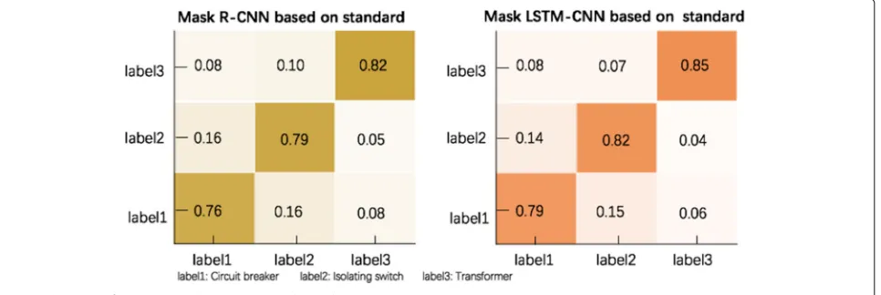
In this section, we use the same rudimentary convolu-tional network and performance parameters to compare the performance of Mask R-CNN and Mask LSTM-CNN.

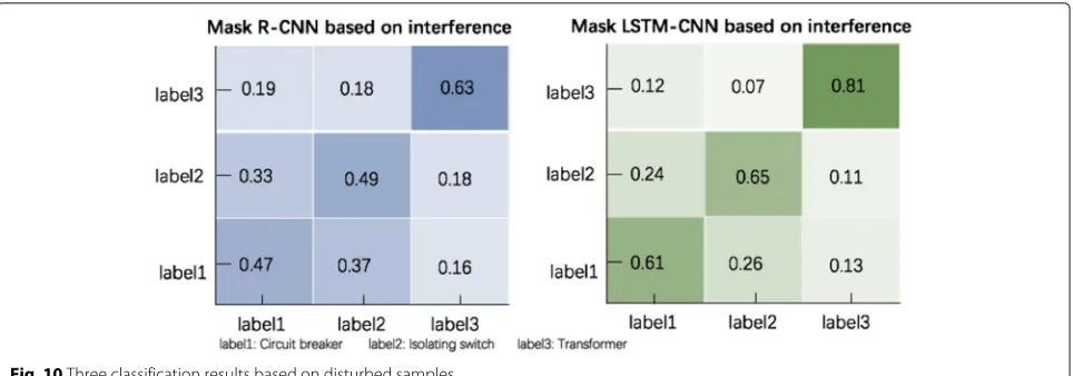
As can be seen in this figure, the proposed method is slightly higher than Mask R-CNN in classification accu-racy of circuit breakers, isolation switches, and trans-formers. To further test the improved advantages of the proposed method, we prepare a particular sample set including 600 power components with shielding, which

are shown in Fig.10. We can see that Mask LSTM-CNN

has a clear advantage over Mask R-CNN in these samples. Figure 11shows the case that there are many obstruc-ters in images. The blue marker is the actual segmentation result of the sample, the red marker is the segmenta-tion result of the Mask R-CNN model, and the green marker is the segmentation result of the Mask LSTM-CNN model. The figure demonstrates that the accuracy of Mask LSTM-CNN segmentation is better than that of Mask R-CNN, and Mask R-CNN identifies more inter-ference backgrounds as part of the target. There are three possible reasons for this exciting phenomenon. The method proposed in this paper incorporates a long-term and short-term memory network before a fully connected decision layer. The method saves the picture information of the upper and lower areas through the intermediate state. The proposed method uses the intermediate state as the input to influence the judgment of the next area. In this way, the proposed model enhances the basis for the model to judge the regional information, and it effectively solves the problem that the model has reduced ability to identify interference factors due to the disappearance of gradients during the training of the model.

Based on the two kinds of samples, further experi-ments are performed to calculate the mAP, mRecall, and mEAO of the two models under different samples. The experimental statistics are in Table 1. In this table, the recognition effect of Mask LSTM-RNN model on normal

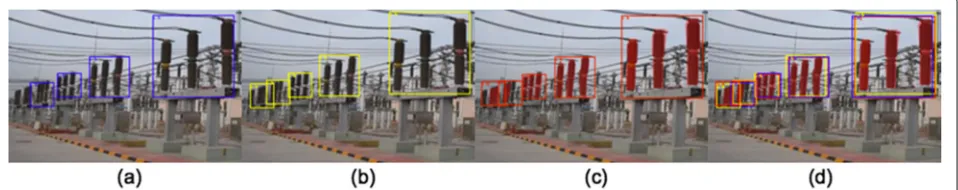
Fig. 13The recognition effect of three models on transformer: (aor blue) Faster-RCNN, (bor yellow) R-FCN, (cor red) Mask LSTM-CNN, and dcomparative results

samples is better than that of Mask R-CNN model. The recognition accuracy of is evidently superior on samples with obstructions. The mAP surpasses Mask R-CNN with an improvement of 16%, mRecall exceeds with a gain of 11%, and mEAO surpasses Mask R-CNN with an increase of 15%.

The power of the site is usually complicated because there are more obstructions before the power component target. Mask LSTM-CNN demonstrates a more significant improvement in this task. The reason is that Mask LSTM-CNN associate ROI information with LSTM before box identification. Through the image information of the nearby areas, it helps to judge the existence of obstacles, strengthens the judgment basis of the neural network, and further improves the accuracy of the classification. And the judgment of the Mask layer depends on the classifica-tion result. The result of the classificaclassifica-tion determines the type of mask that the target generates, so the accuracy of the classification layer directly relates to the accuracy of the Mask.

In addition, we use different basic convolutional frame-works such as VGG, ResNet, and ResNet as the basic network of RCNN and compare the effects of different basic convolutional frameworks on the accuracy of Faster-RCNN, R-FCN, and Mask LSTM-CNN models with the same performance parameters. The classification results and the regional selection of mAP (mean average preci-sion) are shown in Tables2and3.

From Table2, we conclude that the mAP of the model’s underlying network when using ResNet is higher than that of VGG. When the model uses ResNet as the underly-ing network, its map is highest. When the model uses ResNet-101 as the underlying convolutional network, its mAP is as high as 87%. The reason is that ResNet proposes a residual structure compared to VGG. Through reformu-lation, ResNet decomposes a problem into multiple scales and direct residual issues, which can be used to opti-mize the training effect. ResNet retains ResNet’s stack-ing blocks. ResNet splits a sstack-ingle path, simplifystack-ing the model structure and improving computational efficiency.

From the side comparison in Table 2, the LSTM-CNN

of Mask LSTM-CNN has significantly enhanced mAP on Faster-RCNN and R-FCN in three basic convolutions. Because the method proposed in this paper contains the mask layer structure, it enables identification of the model at the pixel level, which ultimately leads to a higher recog-nition rate.

From Table3, the mRecall of Mask-RCNN and R-FCN is

almost equal, which is better than Faster-RCNN. ResNet-101-based Mask LSTM-CNN mEAO is significantly bet-ter than the other two models.

We further compare the time required for the three algorithms to process each image based on the same basic convolutional network. Results in Table4show the R-FCN model has the fastest processing speed. Mask LSTM-CNN is significantly slower than the other two algorithms, but it is also within the acceptable range.

Mask LSTM-CNN is better than Faster-RCNN and R-FCN in both mAP and recall rate. It takes more time to process each picture than the other two models. However,

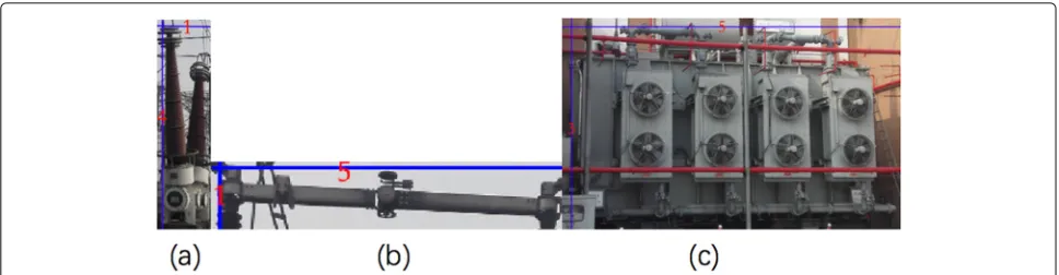
Fig. 15The approximate size of the three targets:acircuit breaker,bisolating switch, andctransformer

Mask LSTM-CNN can refine the detailed profile of com-ponents. It is more conducive to the live working robot to determine the position of the various parts of the parts and the details of the accessories, and it has a better adap-tation to the target shielding. These advantages are due to the alignment between the extracted features and the input of the ROI-Align layer in the Mask-RCNN model. The proposed model uses the matrix instead of vectors to predict each ROI. It reduces the loss of spatial infor-mation. The method proposed in this paper associates the features in the nearby ROI before the fully connected layer. This approach enhances the robustness of object recognition with obstacles. It effectively solves the prob-lem of the gradient disappearing during the process of judging the occlusion object information by a model.

From the following experimental results, as shown in Figs.12and13, the recognition effects of the three models can be seen. The red mark represents the Mask LSTM-CNN, the yellow mark represents the R-FCN, and the blue mark represents the RCNN. Among the Faster-RCNN tagging boxes, the correct number of outer boxes in the target category tag is less than the actual number of outer peripheral boxes. The Mask LSTM-CNN and R-FCN are relatively accurate, and the Mask LSTM-CNN can refine the specific outline of the part.

According to the previously mentioned advantages of Mask LSTM-CNN, we optimize the performance of the

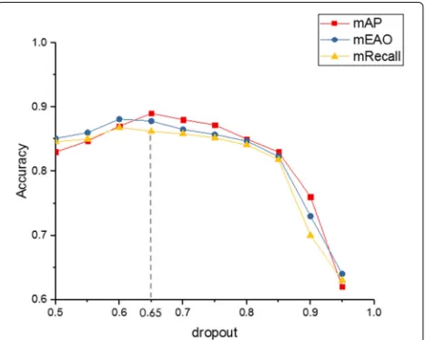
Mask LSTM-CNN model based on ResNet-101. The Mask LSTM-CNN model involves some parameters, such as dropout ratio and nms (non-maximum suppression), and the number and size of the ratio and anchor. These param-eters have a more significant impact on the mAP, and we will discuss them as follows.

Due to the massive time consumption of network train-ing, we only tried 10 different dropouts. As shown in Fig.14, when the dropout ratio increases from 0.5 to 0.95, the accuracy gets the maximum value at approximate 0.65. At present, dropout often depends on experience. We tra-verse according to the specific experimental environment and obtain the relatively optimal value. According to the above experimental results, we set dropout as 0.65 and change the number of anchors. The number of commonly used anchors is set to 9, which belong to three cate-gories and have three aspect ratios (1:1, 1:2, 2:1). Since the scene identified this time is a power accessory, the recog-nition object has a fixed characteristic. According to the size ratio of the power accessories, the anchor is further optimized in this paper.

In experimental results in Fig.15, the size of the isola-tion switch in the area of about 5:1 is more appropriate, while 1:4 for the circuit breaker and 5:3 for the trans-former.

Based on these three ratios, three new dimensions are scaled. This article adds nine new anchors. These

Fig. 17Comparison of the recognition effect of the model to the isolation switch: (aor red) unimproved model, (bor green) improved model, and ccomparative results

nine anchors are used to obtain the various parts of the power device, making us more comprehensive and accu-rate. Further experiments were conducted to compare with the original model. The experimental results are in Figs.16 and17. The red mark indicates that the recog-nition effect of the model is not improved without nine anchors, and the green mark indicates the recognition effect of the improved model with nine anchors. The Mask LSTM-CNN model is more accurate in the area selection of power components, and the contour recog-nition of components is more accurate. In regions with high density of power components, there is a significant improvement in recall rate of recognition. According to

Table 5 (box-map is the average accuracy of the area

recognition, and Mask LSTM-CNN means the average accuracy of the mask), the improved power component recognition model has a noticeable improvement in area selection, contour subdivision, and recall rate.

The model uses a dropout of 0.67 and an anchor type of 18. It changes the image crossover ratio of the nms to IoU and tests its impact on mAP. The result is in Fig.18. According to Fig.18, as the IoU of nms decreases, mAP also gradually decreases. The reason is that the smaller the IoU is, the fewer the candidate areas remain after nms, which leads to a decrease in the accuracy of the detection result. A higher IoU cannot achieve the goal of eliminat-ing the redundancy box by increaseliminat-ing the efficiency of the nms. Therefore, point A in Fig.18corresponds to IoU of 0.86. After point A, the model’s accuracy growth has been slow. Thus, the image of the nms IoU ratio is 0.86.

4.4 Discussion

We have presented corresponding experimental results in above section. The proposed method is compared with several state-of-the-arts, e.g., original Mask R-CNN

Table 5The influence of the number of A on the model

Anchor-number Box-map Mask-map Recall

9 0.886 0.834 0.874

18 0.893 0.867 0.943

method and Faster-RCNN, R-FCN, and other methods. Objectively, since we integrate context features in the classification and regression layers, the proposed method obtains better parameter values, such as mAP, mRecall,

and mEAO. Tables 1, 2, and 3 show that Mask

LSTM-CNN is superior to Mask R-LSTM-CNN, faster-RLSTM-CNN, and R-FCN, and the average accuracy is up to 93%. This demonstrates that our proposed method is more effec-tive. Subjectively speaking, the method proposed in this paper is better than Mask CNN, Faster-RCNN, and R-FCN in identifying power components. Especially when the power components are blocked, the method proposed in this paper is greatly improved in the recognition rate.

Actually, Mask LSTM-CNN can associate ROI informa-tion with LSTM before target classificainforma-tion. A series of convolution operations are performed on the entire image to obtain a feature map: First, generation of a large num-ber of candidate areas on the feature map by the regional proposal network. Next, non-maximum suppression of candidate region boxes, retaining the rst few boxes with higher scores. Then, taking out the feature in the can-didate region frame on the feature map to form a high-dimensional feature vector. Last, calculation of category

recognition and target positioning of the charged detec-tion robot. Even with complicated working condidetec-tions on the scene, the identification accuracy for power compo-nents is still improved greatly. Moreover, we design a long-term and short-long-term memory network to further improve the recurrence of operations and reduce the recognition speed. In the further work, we hope to lower the compu-tational efficiency of the model. A distributed deep neural network may help us to solve this problem. This issue is left as our future work.

5 Conclusions

Based on the analysis of the current and more advanced methods for target detection and identification, this paper verifies the accuracy and efficiency of the recognition of power small parts using Mask LSTM-CNN algorithm. The influence of different parameters on the detection results of Mask LSTM-CNN was analyzed. After combin-ing the features of power components to further optimiza-tion of the model, experiments show that Mask LSTM-CNN model can accurately detect, locate the power com-ponents in real time, and provide a good foundation for automatic maintenance of components in live working robots.

Finally, we point out that a more extensive sample library that can further improve the identification per-formance. In this sense, there may be room for further improvement. Also, a more elaborate identification cate-gory, including the types of fault images for various power components might also be helpful to improve the per-formance. In addition, it is also possible to apply image detection and recognition in other fields. The above three issues are left as our future work.

Abbreviations

AP: Average precision; EAO: Effective area occupancy; Faster-RCNN: Faster region-based convolutional neural network; HOG: Histogram of oriented gradients; LSTM: Long short-term memory; mAP: Mean average precision; mEAO: Mean effective area occupancy; mRecall: Mean recall; NMS:

Non-maximal suppression; R-FCN: Region-based fully convolutional networks; RPN: Regional proposal network; SIFT: Scale-invariant feature transform

Acknowledgements

The authors would like to thank the editors and anonymous reviewers for their valuable suggestions and comments.

Funding

This work was supported by the Natural Science Foundation of China under grant nos. 61672337 and 61472236 and Natural Science Foundation of Shanghai grant no. 16ZR1413100.

and conducted the subjective experiments. FL offered useful suggestions and helped to modify the manuscript. ZL participated in the algorithm design and tested the proposed algorithm. WS conducted the subjective experiment and performed the statistical analysis. All authors read and approved the final manuscript.

Competing interests

The authors declare that they have no competing interests.

Publisher’s Note

Springer Nature remains neutral with regard to jurisdictional claims in published maps and institutional affiliations.

Author details

1_{College of Computer Science and Technology, Shanghai University of Electric}

Power, Shanghai, 200090 People’s Republic of China.2_{Paul G. Allen School of}

Computer Science and Engineering, University of Washington, Seattle, 98105 USA.3_{College of Automation Engineering, Shanghai University of Electric}

Power, Shanghai, 200090 People’s Republic of China.

Received: 29 May 2018 Accepted: 17 September 2018

References

1. J. Y. Park, B. H. Cho, S. H. K. Byun, Development of cleaning robot system for live-line suspension insulator strings. Int. J. Control. Autom. Syst.7(2), 211–220 (2009)

2. C. Liao, J. Ruan, C. Liu, Helicopter live-line work on 1000-kV UHV transmission lines. IEEE Trans. Power Deliv.31(3), 982–989 (2016) 3. C. Chen, J. Wang, H. Zhu, Effects of phasor measurement uncertainty on

power line outage detection. IEEE J. Sel. Top. Sig. Process.8(6), 1127–1139 (2014)

4. S. Fu, Y. Zhang, L. Cheng, Z. Liang, Z. Hou, M. Tan, Motion based image deblur using recurrent neural network for power transmission line inspection robot. inProc. of the JICNN’06 Int. Joint Conf. Neural Netw., 3854–3859 (2006)

5. P. Dehghanian, M. Fotuhi-Firuzabad, S. Bagheri-Shouraki, Critical component identification in reliability centered asset management of power distribution systems via fuzzy AHP. IEEE Syst. J.6(4), 593–602 (2012)

6. Y. Hou, D. I. Jianming, Application of improved scale invariant feature transform accurate image matching in target positioning of electric power equipment. Proc. Csee.32(19), 134–139 (2012)

7. K. Bowyer, C. Kranenburg, S. Dougherty,Edge detector evaluation using empirical ROC curves. Proc. IEEE Conf. Comput. Vision and Pattern Recognition. (Elsevier Science Inc, 2001)

8. N. Dalal, B. Triggs, Histograms of oriented gradients for human detection. inProceedings of the IEEE conference on computer vision and pattern recognition. 886–893 (2005)

9. B. Yangel, D. Vetrov, Image segmentation with a shape prior based on simplified skeleton, Energy Minimization Methods in Computer Vision and Pattern Recognition, St. Petersburg, 247–260 (2011)

10. S. Wei, Q. Hong, M. Hou, Automatic image segmentation based on PCNN with adaptive threshold time constant. Neurocomputing.74(9), 1485–1491 (2011)

11. S. Ren, K. He, R. Girshick, J. Sun, Faster R-CNN: towards real-time object detection with region proposal networks. in Neural Information Processing Systems (NIPS), 91–99 (2015)

13. K. He, G. Gkioxari, P. Dollar, Mask R-CNN. IEEE Int. Conf. Comput. Vis. 2980–2988 (2018). Venice

14. E. J. Kirkland, Bilinear interpolation. Adv. Comput. Electron Microsc. 261–263 (2010). Springer, Boston

15. A. Graves, J. Schmidhuber, Framewise phoneme classification with bidirectional LSTM networks. IEEE Int. Joint Conf. Neural Netw.18(5-6), 602–610 (2005)

16. G. Xu, An adaptive parameter tuning of particle swarm optimization algorithm. Appl. Math. Comput.219(9), 4560–4569 (2013) 17. S. Ren, K. He, R. Girshick,et al, Faster R-CNN: towards real-time object

detection with region proposal networks. IEEE Transactions on Pattern Analysis & Machine Intelligence.39(6), 1137–1149 (2017)

18. R. Girshick, Fast R-CNN. IEEE Int. Conf. Comput. Vis., IEEE, 1440–1448 (2015) 19. J. R. R. Uijlings, K. E. A. V. D. Sande, T. Gevers, Selective search for object

recognition. Int. J. Comput. Vis.104(2), 154–171 (2013)

20. J. Liu, T. Ren, Y. Wang, S. H. Zhong, J. Bei, S. Chen, Object proposal on RGB-D images via elastic edge boxes. NEUCOM.236, 134–146 (2017) 21. L. F. Palafox, C. W. Hamilton, S. P. Scheidt, Automated detection of

geological landforms on mars using convolutional neural networks. Comput. Geosci.101, 48–56 (2017)

22. K. Simonyan, A. Zisserman, Very deep convolutional networks for large-scale image recognition. Int. Conf. Learn. Representations. CoRR, abs/1409.1556 (2014)

23. D. Sarikaya, J. Corso, K. Guru, Detection and localization of robotic tools in robot-assisted surgery videos using deep neural networks for region proposal and detection. IEEE Trans. Med. Imaging.PP(99), 1–1 (2017) 24. J. Koh, M. Suk, S. M. Bhandarkar, A multilayer self-organizing feature map

for range image segmentation. Neural Netw.8(1), 67–86 (1995) 25. B. Sowmya, B. S. Rani, Colour image segmentation using fuzzy clustering

techniques and competitive neural network. Appl. Soil Ecol.11(3), 3170–3178 (2011)

26. N. Dalal, Finding people in images and video. Grenoble Inst. Natl Polytechnique de Grenoble-INPG. (2006)

27. M. Weber, M. Liwicki, D. Stricker, C. Scholzel, S. Uchida, LSTM-based early recognition of motion patterns. in ICPR. IEEE, 3552–3557 (2014) 28. M. F. Stollenga, W. Byeon, M. Liwicki, et al., Parallel multi-dimensional

LSTM, with application to fast biomedical volumetric image segmentation. Comput. Sci. (2015)

29. J. Song, S. Tang, J. Xiao, LSTM-in-LSTM for generating long descriptions of images. Comput. Vis. Media.2(4), 1–10 (2016)

30. M. A. Rafique, W. Pedrycz, M. Jeon, Vehicle license plate detection using region-based convolutional neural networks. Soft. Comput.3, 1–12 (2017) 31. Y. Hirose, K. Yamashita, S. Hijiya, Back-propagation algorithm which varies