(will be inserted by the editor)
EACD: Evolutionary Adaptation to Concept Drifts
in Data Streams
Hossein Ghomeshi · Mohamed Medhat Gaber · Yevgeniya Kovalchuk
Received: date / Accepted: date
Abstract This paper presents a novel ensemble learning method based on evolutionary algorithms to cope with different types of concept drifts in non-stationary data stream classification tasks. In ensemble learning, multiple learners forming an ensemble are trained to obtain a better predictive per-formance compared to that of a single learner, especially in non-stationary environments, where data evolve over time. The evolution of data streams can be viewed as a problem of changing environment, and evolutionary algorithms offer a natural solution to this problem. The method proposed in this paper uses random subspaces of features from a pool of features to create different classificationtypes in the ensemble. Each suchtypeconsists of a limited num-ber of classifiers (decision trees) that have been built at different times over the data stream. An evolutionary algorithm (Replicator Dynamics) is used to adapt to different concept drifts; it allows the types with a higher perfor-mance to increase and those with a lower perforperfor-mance to decrease in size. Genetic Algorithm is then applied to build a two-layer architecture based on the proposed technique to dynamically optimise the combination of features in each type to achieve a better adaptation to new concepts. The proposed method, called EACD, offers bothimplicitandexplicitmechanisms to deal with concept drifts. A set of experiments employing four artificial and five
Hossein Ghomeshi
School of Computing and Digital Technology
Birmingham City Univerity, Birmingham, United Kingdom E-mail: [email protected]
Mohamed Medhat Gaber
School of Computing and Digital Technology
Birmingham City Univerity, Birmingham, United Kingdom E-mail: [email protected]
Yevgeniya Kovalchuk
School of Computing and Digital Technology
real-world data streams is conducted to compare its performance with that of the state-of-the-art algorithms using the immediate and delayed prequential evaluation methods. The results demonstrate favourable performance of the proposed EACD method in different environments.
Keywords Data Streams; Ensemble Learning; Concept Drifts; Evolutionary Algorithms; Genetic Algorithm; Non-stationary Environments
1 Introduction
A considerable effort of recent research has focused on data stream classifi-cation tasks in non-stationary environments [Gama et al., 2014]. The main challenge in this research area concerns the adaptation toconcept drifts, that is, when the data distribution changes over time in unforeseen ways. Con-cept drifts occur in different forms and can be divided into four general types: abrupt (sudden), gradual, incremental and recurrent (reoccurring). In abrupt (sudden) concept drifts, the data distribution at the timet suddenly changes to a new distribution at the timet+1. Incremental concept drifts occur when the data distribution changes and stays in the new distribution after going through some new, unstable, median data distributions. In gradual concept drifts, the proportion of new probability distribution of incoming data in-creases, while the proportion of data that belong to the former probability distribution decreases over time. Recurring concept drifts happen when the same old probability distribution of data reappears after some time of a dif-ferent distribution.
Ensemble learning has proved superiority for stream classification in non-stationary environments over other classification techniques [Gomes et al., 2017a] [Krawczyk et al., 2017]. Ensemble learning is a machine learning ap-proach, in which predictions of individual classifiers are combined using a com-bination rule to predict incoming instances more accurately. The advantage of using ensemble learning techniques in non-stationary data stream classifi-cation lies in their ability to update swiftly according to the most recent data instances. This is usually achieved by training the existing classifiers in the ensemble and changing their weights according to their performance: adding new, better performing classifiers, and removing outdated, low performing classifiers. Applications of classification in non-stationary data streams in-clude spam filtering systems, stock market prediction systems, fraud detection in banking networks, weather forecasting systems, data analysis in Internet of Things (IoT) networks, traffic and forest monitoring systems, among many others. The extensive range of applications makes the task of non-stationary data stream classification even more challenging, as various applications seek diverse purposes and have different conditions.
– Accuracy: the main target of any approach is usually to achieve a min-imum misclassification rate. Hence, the average accuracy rate of an ap-proach should be satisfactory in different evolving data streams.
– Efficiency: in many applications, there are constraints on the system in terms of time and memory usage. When the time calculating an output or the amount of available memory is limited, the learning time and compu-tational complexity of an approach should be minimised.
– Adaptation: when a concept drift happens in a data stream, the accuracy of the ensemble decreases due to the change of the data distribution and the target concept. It is important to minimise the rate of misclassification and the time of recovery upon different types of concept drifts.
The majority of the existing ensemble methods are either focused on one or two of the aforementioned factors, or concentrate on a specific type of data streams. For instance, some approaches do not remove old classifiers [Elwell & Polikar, 2011], [Ramamurthy & Bhatnagar, 2007]; hence, the number of classifiers is unbounded, which can cause a low efficiency in terms of time and memory usage. Other approaches are designed to cope with recurring concept drifts only [Gon¸calves Jr & De Barros, 2013]; therefore, such algorithms are only suitable for a limited number of applications and environments.
To overcome these limitations, we propose a novel ensemble learning method for data stream classification in non-stationary environments, called EACD, that uses random selection of features and two evolutionary algorithms, namely, Replicator Dynamics (RD) and Genetic Algorithm (GA). We train an ensem-ble of different classification types that consist of randomly drawn features (subspaces) of the target data stream. These randomly drawn subspaces are then optimised using GA to cope with different concept drifts over time. Train-ing of the proposed ensemble is performed on sequential data blocks in the stream. The proposed ensemble technique allows a dynamic set of classifica-tiontypesto take action over time. In addition, the number of decision trees in a classificationtype(subspace) depends on the performance of thistypeon the most recent data. Hence, well performingtypes increase in size, while poorly performingtypes decrease in size.
In summary, our solution allows the ensemble to handle different types of concept drifts by employing two different evolutionary techniques. RD is used to continuously determine well and poorly performing types and expand or shrink them accordingly. GA is used to compose new, improvedtypes out of the existing ones by iterating over the most recent data.
2 Related Work
2.1 Ensemble Learning in Non-stationary Data Streams
The majority of the existing data stream learning approaches to non-stationary environments uses ensemble learning techniques for classification tasks [Chu & Zaniolo, 2004a] [Gama et al., 2014] [Gomes et al., 2017a] [Krawczyk et al., 2017], which are more flexible and trustworthy compared to single classifier techniques that use only one classifier for the task.
The existing ensemble methods can be categorised intoexplicit and im-plicit methods. Explicit methods use a concept drift detection mechanism and have an explicit (immediate) reaction to a drift when it is detected, while implicit methods do not have an immediate reaction to concept drifts, and as such, adapt to drifts implicitly by updating the state of the ensemble according to the most recent instances.
Implicit Methods
Online bagging (OzaBag) [Oza, 2005] is an online version of bagging learning mechanism that can be used in data streams (as opposed to the standard bagging technique that requires the training set to be available at once). It updates each classifier in the ensemble with k copies of the newly received instances. The value ofkcomes from the Poisson distributionP oisson(1).
Online boosting (OzaBoost) [Oza, 2005] is an online version of the boosting learning mechanism. In this method, every new example received by the en-semble is used to update all classifiers in a sequential manner. In other words, the first classifier is assigned with the highest possible weight for the newly received data, while the weights assigned to the next classifiers are based on the outcome of the previous classifiers.
OSBoost [Chen et al., 2012] is an algorithm that uses online boosting and combines weak learners by producing a connection between the online boosting and the batch boosting algorithms. It is theoretically proved to achieve a small error rate, as long as the number of weak learners and the number of examples are sufficiently large.
Dynamic Weighted Majority (DWM) [Kolter & Maloof, 2007] is an implicit approach, where data come in an online form and get classified immediately. If a classifier misclassifies an instance after a predefined period (p instances), the weight of this classifier is reduced by a constant value regardless of the ensemble’s output and all weights are normalised. Then, the classifiers with the weights lower than a predefined threshold (θ) are removed from the ensemble. Finally, when the whole ensemble misclassifies an instance, a new classifier is built and added to the ensemble. All classifiers are trained incrementally with incoming samples.
on their error in a constant time and memory. In this algorithm, the incremen-tal nature of Hoeffding trees [Domingos & Hulten, 2000a] is combined with a normal block-based weighting mechanism. This approach does not remove any old classifiers; therefore, a threshold for memory is assigned so that whenever it is met, a pruning method is used to reduce the size of classifiers. An online ver-sion of this approach (OAUE) was introduced by the same authors [Brzezinski & Stefanowski, 2014a].
Anticipative Dynamic Adaptation to Concept Changes (ADACC) [Jaber, 2013] is an implicit method that attempts to optimise stability of the ensemble by recognising incoming concept changes. This is achieved by establishing an enhanced forgetting strategy for the ensemble. ADACC takes snapshots of the ensemble when a concept is recognised asstable and uses them when there is instability in the system to cope with concept drifts.
Social Adaptive Ensemble (SAE) [Gomes & Enembreck, 2013] is a method that has the same learning strategy as the DWM algorithm. It maintains an ensemble that is arranged as a network (undirected graph) of classifiers. Two classifiers are connected to each other when they produce similar predictions. These connections are weighted according to a similarity coefficient equation. The ensemble is updated after a predefined number of instances. The same au-thors extended their method toSAE2 approach [Gomes & Enembreck, 2014]. The main issue with implicit methods is that in most cases adaptation to a new concept takes a long time due to their implicit behaviour. Furthermore, concept drifts are not identified immediately with such approaches.
Explicit Methods
Adaptive Boosting (Aboost) [Chu & Zaniolo, 2004b] is one of the approaches that uses a concept drift detection method. It builds one classifier per every block of data that is received from the stream and classifies the instances. Then, it evaluates the ensemble’s output and updates the weights of all classifiers based on whether or not an instance is classified correctly by the ensemble, as well as the classifier itself. Whenever a concept drift is detected, the weight of each classifier in the ensemble is reset to one. Finally, once the size of the ensemble is exceeded, the oldest classifier is removed from it.
Adwin Bagging (AdwinBag) [Bifet et al., 2009] is an approach that uses Oza’s online bagging algorithm [Oza, 2005] for its learning mechanism and adds a concept drift detector called ADaptive WINdowing (ADWIN) [Bifet & Gavalda, 2007] to specify when a new classifier is required. AdwinBag is enhanced in the Leveraging Bagging (LevBag) algorithm [Bifet et al., 2010b] by the same authors. LevBag aims to add randomisation to the input and the output of the classifiers and increase the extent of re-sampling in the bagging technique. The re-sampling rate in LevBag is changed from P oisson(1) to P oisson(λ), whereλis a user defined parameter.
stream. This framework contains a two-phase concept drift detection mecha-nism. First, a new classifier is created and trained alongside a new buffer when the drift detection mechanism signals a warning. If it then signals a drift, which means the concept drift is approved, the system checks whether or not the new concept is similar to another concept that has been previously stored in the buffer. If there has been a recurring concept drift, RCD uses the classifier created with that concept drift to classify the incoming data and then starts training the classifier. If no similar concept drift is found in the buffer, RCD stores the newly trained buffer and the classifier in the system and uses them to classify the incoming instances. If the system does not get the drift signal to approve the drift, it assumes it to be a false alarm; the system ignores the stored data and continues to classify using the current classifier. Note, only one classifier is activated at a time in this approach, while the rest are deactivated, unless the same data concept happens again.
Adaptive Random Forest (ARF) [Gomes et al., 2017b] is an explicit en-semble learning technique, which is an adaptation of the classical Random Forest algorithm [Breiman, 2001] that grows decision trees by training them on re-sampled versions of the original data and by randomly selecting a small number of features that can be inspected at each node for split. ARF is based on a warning and drift detection scheme per tree, such that after a warning has been detected for one tree, another one (background tree) starts growing in parallel and replaces the original tree only if the warning escalates to a drift. In summary, the main issue with explicit methods is their sensitivity to false alarms (noise). Therefore, accuracy of the system using such methods can be degraded severely by a wrongly detected concept drift. Furthermore, employing a good drift detection mechanism that can recognise different types of concept drifts (gradual, recurring, abrupt and incremental) [Gama et al., 2014] is a difficult task. In this scenario, RD offers a smooth yet effective way to improve the performance of the ensemble by increasing or reducing the number of trees in classification types. Furthermore, the main issue with implicit algorithms is their slowness in coping with concept drifts as they do not have an immediate reaction to drifts. This is the reason for using a concept drift detection algorithm along with GA to immediately react to concept drifts and to optimise the combination of the features in classificationtypes. Overall, by combining RD with concept drift detection methods and GA, it is feasible to have the advantages of explicit and implicit methods alongside in the ensemble.
2.2 Evolutionary Algorithms in Non-stationary Data Streams
The StreamGP algorithm [Folino et al., 2007] builds an ensemble of clas-sifiers using Genetic Programming along with the boosting algorithm to gen-erate decision trees, each trained on different parts of the data stream. This algorithm is an explicit algorithm that uses a concept drift detection mecha-nism. Whenever a concept drift is detected, a new classifier is created using CGPC [Folino et al., 2006], which is a cellular genetic programming method that generates a classifier as a decision tree. Each population in this algorithm is a set of individual data blocks (nodes) that initially is drawn randomly. The newly created classifier is then added to the ensemble and all classifiers are boosted by updating their weights. This algorithm is different from our pro-posed algorithm in that in StreamGP, the aim of the optimisation technique is to find the best set of data blocks to create a new classifier. InEACD how-ever, the aim of GA is to find the best combination of features to create new classification types. Unlike our method, the problem with StreamGP is that no new classifier is created by the system unless a concept drift is detected. This might negatively affect the performance upon incremental and gradual concept drifts that are hard to detect.
Online Genetic Algorithm (OGA) [Vivekanandan & Nedunchezhian, 2011] is a rule-based learning algorithm that builds and updates a set of candidate rules for a data stream based on the evolution of the data stream itself. In this algorithm, the rules are initially set randomly, and after fully receiving a new data block, an iteration of GA is performed to search for new (better) candi-date rules for all classes in the received data block. This process is repeated until the end of the stream. The differences between OGA and our proposed algorithm are as follows. Primarily, OGA is a rule-based learning algorithm, whereas EACD is an ensemble learning algorithm. The aim of GA in OGA is to create new rules or update the current rules, whereas the aim of GA in EACDis to optimise the classificationtypesinside the ensemble. Furthermore, the iterations in OGA are performed over different data blocks (an iteration per each data block) and GA never stops its iterations (the maximum number of generations is unlimited), whereas in EACD, the iterations are performed over the same fixed data in the buffer for each round of GA, and the number of generations is limited. The main issue with OGA is the long time it takes to adapt to new concept drifts since GA takes only one data block at each iteration, potentially requiring a large number of iterations to completely cope with a concept drift.
3 Proposed Method
3.1 Replicator Dynamics: An Overview
next selection is given by the replicator equation as a function of the type’s payoff and its current proportion in the population’ [Fawgreh et al., 2015]. In other words, atype’sexpected payoff is determined by the payoff matrix, and hence, the population of each type is determined according to its expected payoff. The types that score above the average payoff increase in population, while the types that score below the average payoff decrease in population. TheReplicator Equation is represented by the following formula:
˙
xi=xi[(W x)i−xTW x], (1)
where (W x)iis the expected payoff for an individual andxTW xis the average payoff in the population statex.
In our proposed method, a type (classification type) is a subspace of the total number of features of the target data stream that initially is drawn ran-domly and then is being optimised using GA. A type’s payoff is the average accuracy of the classifiers that have been built using the specifiedtype (sub-space of features). The expected payoff is the average accuracy of all classifiers in the ensemble.
3.2 Genetic Algorithm: An Overview
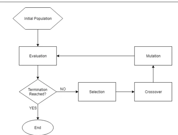
GA is a meta-heuristic algorithm inspired by the process of natural selection, which is a subset of a bigger class of algorithms called evolutionary algo-rithms. Such algorithms are commonly used to generate high-quality solutions to optimisation and search problems relying on bio-inspired operators such as mutation, crossover andselection. The reason for using GA in the proposed method is that GA is superior to other optimisation methods when there are a relatively large number of local optima [Elyan & Gaber, 2017], which is the case in this problem, where numerous subspaces of features likely to form ‘types’ can form local optima.
Fig. 1 An illustration of a typical Genetic Algorithm.
3.3 EACD: Evolutionary Adaptation to Concept Drifts
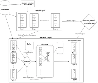
We propose a novel ensemble learning algorithm that is suitable for non-stationary data stream classification. In this algorithm, the data come as con-tinuous data blocks. In this paper, each data block consists of 1,000 samples that are selected arbitrarily; however, it can be set to any other values as re-quired. The algorithm comprises of two different layers called the base layer and thegenetic layer. Each layer has a set of classifiers that classify the incom-ing data independently. The base layer is always active, whereas the genetic layer is only active when GA has made its generations and thetypes are ma-ture enough. The classifiers that comprise the second (genetic) layer have more weight than the classifiers comprising the base layer to achieve optimality of the types.
The base layer is built using random selection of features and gets ex-tended using RD. The genetic layer is built by applying the GA optimisation technique to the set of features randomly selected from the base layer and introduces a new set of classificationtypes that gets optimised by the recent instances stored in the buffer. Both the base and the genetic layers are detailed in the following subsections. In addition, Figure 2 illustrates how the proposed algorithm works.
such drifts or detect them with a delay. In this scenario, RD offers a smooth yet effective way to improve the performance of the ensemble by increasing and reducing the number of trees in the classificationtypes. Furthermore, the main problem with the implicit algorithms (the ones without a concept drift detection mechanism) is their slowness in coping with concept drifts as they do not have an immediate reaction to drifts. This is the reason for using a concept drift detection algorithm along with GA to immediately react to concept drifts and optimise the combination of the features in classificationtypes. Overall, by combining RD with concept drift detection methods and GA, it is feasible to have the advantages of explicit and implicit methods alongside in the ensemble, as previously discussed in Section 2.
Fig. 2 Architecture of the proposed EACD algorithm.
3.3.1 Base Layer
com-patible with non-stationary environments and to seamlessly adapt to the most current types of data and concepts. In other words, RD is used to increase the number of well-performing classification trees and reduce the number of unhelpful ones.
The base layer is built using the following steps. First, p percent of all features are randomly selected from the pool of data features (attributes) of the target data stream. This phase is calledrandom subspace. In other words, the total number of features that is to be selected randomly from the pool of features is established as:
n= p
100×f, (2)
where n is the total number of features that needs to be selected, p is an arbitrary number (0 < p < 100) that shows the percentage of the features that should be selected randomly andf is the total number of features of the target data stream. Each iteration of this step produces a set of randomly selected features (subspace) from the pool of features that we call atype. This step is repeatedmtimes; hence, there aremindependent classificationtypesat the end of this step. Note thatmis a parameter of our proposed model for the total number of classificationtypesin the ensemble and is chosen depending on the total number of features of the target stream; there should be a balance between the number of types (m) and the number of features in each type (p×f).
Next, a decision tree is built per every classificationtype (subspace) when the first block of data (samples) is received by the system. Given the maximum number of classifiers for each type max, this step is repeated for the first
max
2 data blocks received by the system for the types to shape and reach a specific maturity level. This phase is called theinitial training, during which, an average number of classifiers for everytype in the ensemble is built. Note that for every data block received by the ensemble, all decision trees classify the instances and the majority voting then determines the ensemble’s output. This is called thevoting step.
Once the initial training phase is completed, each decision tree is evaluated after classifying incoming instances. The accuracy (a) of each decision tree in atype is calculated as:
ai= ci
db, (3)
where ci is the number of correctly classified instances inithdata block and dbis the total number of instances in each data block. Accuracy of eachtype is the average accuracy of its related decision trees. Accuracy of the whole ensemble can be determined similar to Equation 3. This phase is called the evaluation phase.
fixed number. The types with a higher payoff (accuracy) than the expected payoff get a new decision tree (i.e. a new decision tree is built for such data types based on the last block’s samples), whereas thetypes with a lower payoff (accuracy) than the expected payoff lose a decision tree. In other words,
a(ti)≥ Pm
i=1a(ti)
m ⇒grow
a(ti)< Pm
i=1a(ti)
m ⇒shrink
, (4)
wherea(ti) is the accuracy of theithtypeandmis the total number oftypes. Finally, every decision tree in the ensemble is trained with the samples from a newly received data block in theretraining phase. The purpose of this phase is to have a more updated ensemble, especially when a concept drift happens. In this situation, retraining can lead to a fast adaptation since all classifiers are trained with the newly evolved data.
To limit the size of the ensemble, an upper bound for the number of decision trees (classifiers) in a type is assigned. When the maximum size of a type is exceeded, the least performing decision tree of that specific type is removed. The upper bound (max) for the number of classifiers in this paper is set to the arbitrary value of max= 20. Furthermore, a lower bound (min) is assigned to all types to prevent the types from complete removal. In this paper, the minimum size of alltypesis set tomin= 1. Hence, a tree is not removed upon poor performance if it is the only one decision tree related to a type left.
Algorithm 1 shows how the base layer is built and works. In this algorithm, tj is thejthtypeof the ensemble (1≤j≤m) anda(tj) is the accuracy of this type. The following functions are used in the presented algorithm:
– Classify(): the ensemble classifies data using the majority voting;
– Evaluate(): evaluate the accuracy of alltypes in the ensemble using Equa-tion 3;
– Grow(): add a new classifier (decision tree) to the specifiedtype(if Equation 4 stands);
– Shrink(): remove one classifier (decision tree) from the specifiedtypebased on the ensemble’s removal mechanism (if Equation 4 stands); if this type has only one classifier, then do nothing;
– Train(): train all classifiers using the samples from the newly received data block.
In the presented algorithm, lines 2 and 3 refer to therandom subspace phase. Lines 5, 6 and 7 are theinitial training phase. Theevaluation phase is imple-mented in line 10, theRD phase is in lines 11 to 14, and finally, theretraining phase is in line 15. Decision trees are removed based on their performance; the tree that performs the worst in the specifiedtype is removed.
3.3.2 Genetic Layer
Algorithm 1: EACD Base Layer
Input:A continuous block of data,DB={db1,db2,..,dbn}
n: number of features that should be selected in eachtype
m: total number oftypes
max: maximum number of classifiers in eachtype.
Output:Classified Samples 1 i:= 1
2 fort:= 1tot:=mdo 3 Randomly selectnfeatures 4 whiledata stream is not emptydo
5 if i≤ max
2 then
6 Classify(dbi)
7 Grow(T) for all thetypes
8 else
9 Classify(dbi)
10 Evaluate()
11 if a(tj)≥
Pn j=1a(tj)
m then
12 Grow(tj)
13 else
14 Shrink(tj)
15 Train() 16 i:=i+ 1
(subspaces) as its input and tries to form the best possible combination of the features in eachtype. This is achieved by iterating over a fixed data that has been received by the system recently (buffer). The genetic layer is different from the base layer only in this part (i.e. the combination of classification types), whereas the classification, training and updating mechanisms are the same as explained for the first layer.
Algorithm 2 shows how the genetic layer is being built. First, the set of randomly drawn subspaces is taken from the base layer and considered as the first GA population. Note that in this algorithm, each classificationtypeis con-sidered as anindividual in GA, and each feature inside atypeis achromosome of thisindividual.
The buffer always keeps the most recently labelled instances received by the system. It serves as a search space for the GA optimisation task. Whenever GA starts or restarts, it copies the data inside the buffer into the memory and uses them for its procedures, i.e. theselection stage and the fitness function.
Selection stage:for every GA iteration, the classificationtypes that have a better accuracy than the overall average accuracy of alltypes over the search space are selected for the crossover stage. Hence, the GA fitness function is thetypes’ average accuracy over the search space. Algorithm 2 refers to this part with “Selection()” function.
other well performingtypes to make offspring. Algorithm 2 refers to this part with “Crossover()” function.
Mutation stage: the mutation rate of 5% applies upon breeding of the types. Hence, there is a 5% chance for an offspring to get a random feature from the pool of features instead of getting all of them from its parents. Algorithm 2 refers to this part with “Mutation()” function.
When the maximum number of generations is achieved, the resulting clas-sification types form a new set of classifiers that starts to be trained and evaluated with incoming data. The new ensemble model is said to be mature enough when its performance on the latest data block is better than the av-erage performance of the algorithm. As mentioned before, the base layer is always active, whereas the genetic layer is active when the GA has done its job and the layer has reached its maturity level. All classifiers inside the base layer of the proposed algorithm are given the arbitrary weight of one (Wb= 1), whereas all classifiers inside the genetic layer are given the arbitrary weight of two (Wg= 2). This intensifies the effect of the genetic layer on the algorithm given the optimality of the types.
Once a new data block is received by the system, it goes to both layers, and the classifiers inside each layer classify the instances and send their predictions to the decision making part of the algorithm independently (as illustrated in Figure 2). The decision maker then considers all the received predictions from the active classifiers and performs the voting procedure according to the weight of each prediction. This decision maker also tracks and keeps the average accuracy of each layer in the algorithm. Whenever GA is due to restart its procedures, the genetic layer is deactivated and cleared to make room for the new set oftypes. To determine when to start a new set of GA generations (i.e. reset the genetic layer), one implicit and one explicit mechanisms are proposed in this paper.
Algorithm 2 refers to theConcept Drift Detectionpart with ”DriftDetector()” function.
Algorithm 2: EACD Genetic Layer
Input:Buffer
g: Maximum number of generations Resetting mechanism: [implicit/explicit]
Randomly drawn subspaces (types) from the base layer,TB={t1,t2,..,tm}
Output:New set of classificationtypes,TG={t10,t20,..,tm0}
1 fori:= 1toi:=gdo
2 Selection() 3 Crossover() 4 Mutation()
5 if Resetting mechanism=Implicit then 6 repeat
7 Evaluate(TB) /*Evaluates base layer over the last 10 data blocks*/
8 Evaluate(TG) /*Evaluates genetic layer over the last 10 data blocks*/
9 untilAverage accuracy (TG)≤Average accuracy (TB)
10 Reset(GA) /*Clear the genetic layer and restart GA*/
11 else
12 repeat
13 DriftDetector()
14 untilDriftDetector()=Drift /*when the detector signals a drift*/ 15 Reset(GA) /*Clear the genetic layer and restart GA*/
3.4 Theoretical Justification
In the literature of mining non-stationary data streams, there is no deter-ministic method that can guarantee to find the global optima. This is due to the evolving nature of the data that come in the form of a stream. Hence, a single classifier of a data stream that is optimal in a specific environment can become the worst classifier once the data has evolved in the same data stream. By adding randomisation to create different classificationtypes in the first layer of the proposed method, it is feasible to have a variety of classifiers in the ensemble. This leads to a diverse set of available solutions to quickly cope with an occurring concept drift. However, having different classification types can also cause problems such as degrading the accuracy in case of using one or more poortypes. This problem is tackled by employing RD to increase the number of well-performingtypes and reduce the number of low-performing ones in the base layer of the proposed algorithm.
is a powerful and broadly applicable stochastic optimisation technique [Gen & Cheng, 2000] that can be used in dynamic environments (e.g. data streams) after adding a few changes to its mechanism, as was proposed in this paper.
4 Experimental Study
To evaluate the proposed algorithm, a set of experiments is conducted using nine datasets comprising of four artificial (synthetic) data stream generators and five real-world data streams. We compare the EACD algorithm to the state-of-the-art ensemble methods for non-stationary data stream classifica-tion that have shown a good performance and reliable results [Brzezinski & Stefanowski, 2014a] [Gomes et al., 2017b], including Dynamic Weighted Ma-jority (DWM) [Kolter & Maloof, 2007], Online Accuracy Updated Ensem-ble (OAUE) [Brzezinski & Stefanowski, 2014a], OSBoost [Chen et al., 2012], Leveraging Bag (LevBag) [Bifet et al., 2010b] and Adaptive Random Forest (ARF) [Gomes et al., 2017b].
EACD is developed in Java programming language using the Massive On-line Analysis (MOA) API [Bifet et al., 2010a]. All other algorithms are already included in the MOA framework [Bifet et al., 2010a], which is used as the experimental environment here. MOA is an open source framework for data stream mining in evolving environments. When running LevBag, ARF, DWM, OAUE and OSBoost, their default parameters as set in MOA are used, while the parameters for running the proposed algorithm are listed in Section 4.2.
To have a thorough set of experiments with precise results, 10 different variants for every artificial data stream are generated and each method is tested on all variants. These variants are generated by changing different pa-rameters in all artificial streams. The selected papa-rameters for each data stream generator are specified later in Section 4.1. For every real-world data stream, each experiment is repeated 10 times over the same data stream.
Hoeffding trees are used in the experiments as the base classifiers (decision trees). Hoeffding tree, also known as the Very Fast Decision Tree (VFDT) method [Domingos & Hulten, 2000a], is an incremental decision tree algorithm that is capable of learning from massive data streams.
The experiments were performed on a machine equipped with an Intel Core i7-4702MQ CPU @ 2.20GHz and 8.00 GB of installed memory (RAM).
4.1 Datasets
4.1.1 Artificial Data Streams
The following four artificial data stream generators are employed to simulate data for the experiments: the SEA generator, the Hyperplane generator, the Random Tree (RT) generator and the LED generator. Ten different stream variants are created for each of the considered data generators using their respective parameters to examine the performance of the tested algorithms depending on the type of the concept drifts. In case of the SEA generator, the variants are built by changing the random seed along with the type of man-ually added concept drifts. For the Hyperplane generator, different variants are built by tweaking the number of drifting attributes and the magnitude of changes in data. For the RT generator, the random seed number along with the number of attributes and classes are changed. Finally, for the LED gener-ator, different variants are built by tweaking the number of drifting attributes and the random seed number.
SEA Generator
The SEA generator [Street & Kim, 2001] is a synthetic data stream generator that aims to simulate concept drifts over time. It generates random points in a three-dimensional feature space; however, only the first two features are relevant.
In case of the SEA generator, each variant includes one million instances. In addition, different concept drifts are manually chosen to happen in the instance numbers 200K, 400K, 600K and 800K. For the first five variants, two abrupt concept drifts with a width (width of concept drift change) of one are added at the instance numbers 200K and 400K, and two recurrent concept drifts with the same width are added at the instance numbers 600K and 800K. For the remaining five variants, two gradual concept drifts with a width of 10,000 are added at the instance numbers 200K and 400K, and two recurrent concept drifts with the same width are added at the instance numbers 600K and 800K.
Hyperplane Generator
Table 1 The number of drifting attributes and the magnitude of change selected for differ-ent stream variants based on the Hyperplane generator.
Variant No. of drift-ing att.
Mag. of change
Variant No. of drift-ing att.
Mag. of change
1 2 0.01 2 2 0.02
3 3 0.01 4 3 0.02
5 4 0.01 6 4 0.02
7 5 0.01 8 5 0.02
9 6 0.01 10 6 0.02
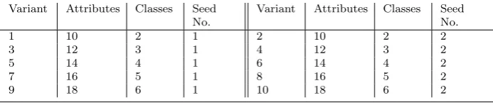
Table 2 Total number of attributes, number of classes and random seed number of different stream variants based on the RT generator.
Variant Attributes Classes Seed No.
Variant Attributes Classes Seed No.
1 10 2 1 2 10 2 2
3 12 3 1 4 12 3 2
5 14 4 1 6 14 4 2
7 16 5 1 8 16 5 2
9 18 6 1 10 18 6 2
changing the location of the hyperplane. The smoothness of drifting data can be changed by adjusting the magnitude of the changes.
In the presented experiments, the number of classes and attributes are set to two and ten, respectively, and the number of drifting attributes and the magnitude of changes are set as indicated in Table 1. The number of instances in each stream is set to one million.
Random Tree Generator
The RT generator [Domingos & Hulten, 2000b] builds a decision tree by ran-domly selecting attributes as split nodes and assigning random classes to them. After the tree is built, new instances are obtained through the assignment of uniformly distributed random values to each attribute. The leaf reached after a traverse of the tree determines its class value according to the attribute values of an instance. The RT generator allows customising the number of nominal and numeric attributes, as well as the number of classes. In the experiments, the number of classes, the number of features and the random seed number are chosen as indicated in Table 2.
LED Generator
LED generator is used to simulate concept drifts by swapping four of its fea-tures resulting in ten different stream variants. For the first five variants, the number of drifting attributes are chosen to be 1, 2, 3, 4 and 5, respectively. For the next five variants, only the random seed is changed, while the drifting attributes remain the same as in the first five variants.
4.1.2 Real World Data Streams
Forest Cover-type Dataset
The Forest Cover-type data stream [Blackard & Dean, 1999] is a real world dataset from the UCI Machine Learning Repository1. It contains the forest cover type of 30×30 meter cells obtained from the US Forest Service (USFS). It consists of 581,012 instances and 54 attributes. The goal in this dataset is to predict the forest cover type from cartographic variables.
Electricity Dataset
Electricity is a widely used dataset by [Harries & Wales, 1999] collected from the Australian New South Wales electricity market. In this market, prices are not fixed and affected by demand and supply. The Electricity dataset contains 45,312 instances. Each instance contains eight attributes, and the target class specifies the change of the price (whether it goes up or down) according to its moving average over the last 24 hours.
Airlines Dataset
Airlines2is a regression dataset. The task is to predict whether a flight will be delayed providing the information on its scheduled departure. This dataset has two classes (whether a flight is delayed or not) and contains 539,383 records with seven attributes (three numeric and four nominal).
Poker-Hand Dataset
The Poker-Hand dataset from the UCI Machine Learning Repository3 con-sists of 1,000,000 instances and 11 attributes. Each record of the Poker-Hand dataset is an example of a hand consisting of five playing cards drawn from a standard deck of 52. Each card is described using two attributes (suit and rank), with a total of 10 predictive attributes. There is one class attribute that describes the “poker hand”.
1 http://archive.ics.uci.edu/ml 2 http://kt.ijs.si/elena
ikonomovska/data.html
KDDcup99
KDDcup99 [Cup, 1999] is the dataset used in the “Third International Knowl-edge Discovery and Data Mining Tools Competition”. The competition task was to build a network intrusion detector – a predictive model capable of distinguishing between “bad” connections (intrusions or attacks) and “good” (normal) connections. KDDcup99 contains a standard set of data to be au-dited, which includes a wide variety of intrusions simulated in a military net-work environment. This dataset contains 41 attributes and 23 classes.
4.2 EACD Variations
Eight different variations of the proposed algorithm are implemented and com-pared in the experiments to evaluate the impact of each EACD characteristic and discuss the effect of employing different parameters in the EACD algo-rithm. Thebase variations only use the base layer of the proposed algorithm, while GA optimisation is not applied; only base4 variation uses the concept drift detector to restart the layer upon drifts. The implicit (Imp) variations use an implicit mechanism, whereas the explicit (Exp) variations use an explicit mechanism to specify when the genetic layer should be restarted (as explained in Section 3.3.2). The specific parameters of the eight proposed variations are as follows:
– EACDbase: p= 60% andm= 0.6×f;
– EACDbase2: p= 30% andm= 0.3×f;
– EACDbase3: p= 60% andm= 0.3×f;
– EACDbase4:p= 60%,m= 0.6×f and restarting the ensemble upon drifts;
– EACDImp:g= 15,z= 5%,p= 60% and m= 0.6×f;
– EACDImp2:g= 15,z= 5%,p= 60%, m= 0.6×f;
– EACDExp:g= 15,z= 5%,p= 60%,m= 0.6×f;
– EACDExp2:g= 15,z= 0%,p= 60%,m= 0.6×f,
wherepis the number of features in each classificationtype,mis the number of classificationtypesin the layer,f is the total number of features in the data stream,gis the total number of generations for each GA iteration andzis the mutation rate of GA.
4.2.1 Computational Complexity
fact that RD uses m arithmetic operations to calculate payoffs, the cost of applying RD to the ensemble is only O(m). Hence, the time complexity of de-ploying the base variations of the proposed method (EACDbase,EACDbase2 andEACDbase3) is O(m+ (kcvp)).
Assuming the size s of the GA population and the total number of gen-erations g, the cost of GA optimisation is O(sg) at each time when the ge-netic layer needs to be restarted. Hence, the time complexity of deploying the implicit variations of the proposed method (EACDImp and EACDImp2) is O(m+ (kcvp) + (sg)).
Finally, givendas the number of instances in each data block andf as the total number of features in the dataset, the EDDM drift detection method, which uses J48 (C4.5) decision tree as its learning mechanism, requires O(df2) of time. Hence, the time complexity of deploying the explicit variations of the proposed method (EACDExpandEACDexp2) is O(m+ (kcvp) + (sg) + (df2)). Note that the cost of running evolutionary methods is minimised providing the variations applied to EACD as previously discussed.
4.3 Results
The considered algorithms are compared using standard criteria, including the classification accuracy and the overall time. There are two settings for each experiment (immediate and delayed) as explained previously in this section.
Tables 3 and 4 show the average accuracy for the proposed EACD vari-ations over the mentioned nine datasets in the immediate and the delayed settings, respectively. As can be seen from the tables,EACDExphas the best average accuracy over the Hyperplane, the LED, the SEA, the Airlines, the Electricity and the Poker-Hand datasets. It also has the best overall average accuracy in both the immediate and the delayed settings.EACDImp has the best average accuracy over the Forest Cover-type and the RT datasets, wheras EACDExp2has the best average accuracy over the KDDcup99 dataset.
As the difference betweenEACDImpandEACDImp2is in their number of generations used in each GA iteration, their accuracy is not significantly differ-ent, andEACDImp, which has a higher number of generations (15), performs better over all datasets. It is clear that the evaluation time of EACDImp2 is less than that ofEACDImp since GA performs faster on 10 generations com-pared to 15 generations. Similarly, as the difference between EACDExp and EACDExp2 is in their GA mutation rate parameter, they both have compa-rable accuracy and execution time, and only EACDExp accuracy is slightly better for the majority of the datasets.
vari-Table 3 Average accuracy (%) of the EACD variations in the immediate setting. Dataset base base2 base3 base4 Imp Imp2 Exp Exp2
Hyper. 86.31 77.47 80.52 84.74 89.23 88.54 90.59 90.53
LED 68.78 63.05 64.12 67.75 74.78 74.02 75.45 75.42
RT 88.03 79.34 86.34 89.93 91.89 91.23 91.42 91.41
SEA 87.35 82.43 84.56 88.90 87.43 85.78 90.08 90.00
Airlines 62.97 60.09 61.78 62.08 64.37 63.98 66.61 66.60
Elec. 81.01 77.34 80.45 81.76 90.30 90.23 92.14 92.10
Forest 83.56 70.34 80.67 85.83 92.64 91.94 91.73 91.73
KDDcup 99.76 98.67 98.89 99.76 99.76 99.76 99.78 99.79
Poker 80.24 73.45 75.23 79.51 83.45 82.78 86.21 86.17
Overall Average
82.00 75.80 79.17 82.25 85.98 85.36 87.11 87.08
Table 4 Average accuracy (%) of the EACD variations in the delayed setting. Dataset base base2 base3 base4 Imp Imp2 Exp Exp2
Hyper. 84.35 75.34 78.23 83.40 88.43 88.05 90.02 89.98
LED 68.17 62.67 64.00 67.69 73.60 73.14 75.26 75.25
RT 87.16 79.02 84.23 87.92 91.24 90.20 91.05 91.01
SEA 85.94 80.56 82.43 87.38 87.06 85.24 89.22 89.20
Airlines 60.45 56.07 58.12 62.48 62.18 62.56 63.35 63.14
Elec. 74.35 73.67 84.35 75.01 83.32 84.35 85.03 84.97
Forest 79.45 70.34 79.23 80.05 85.90 85.34 84.83 84.80
KDDcup 99.76 98.67 98.84 99.75 99.75 99.76 99.76 99.77
Poker 77.92 70.78 73.37 76.90 78.03 77.45 80.21 79.24
Overall Average
79.73 74.12 78.09 80.06 83.28 82.90 84.30 84.15
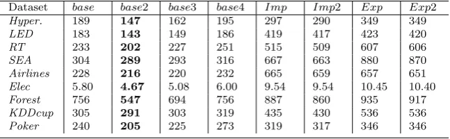
Table 5 Average evaluation time (in seconds) of executing the EACD variations.
Dataset base base2 base3 base4 Imp Imp2 Exp Exp2
Hyper. 189 147 162 195 297 290 349 349
LED 183 143 149 186 419 417 423 420
RT 233 202 227 251 515 509 607 606
SEA 304 289 293 316 667 663 880 870
Airlines 228 216 220 232 665 659 657 651
Elec 5.80 4.67 5.08 6.00 9.54 9.54 10.45 10.40
Forest 756 547 694 756 887 860 935 917
KDDcup 305 291 303 319 435 430 536 536
Poker 240 205 225 273 319 317 346 346
ations are similar as their only difference is in the GA mutation rate, which does not affect the times severely. Note that the evaluation times do not have significant difference in the immediate and the delayed settings; hence, only the evaluation times of the immediate setting are shown in this paper.
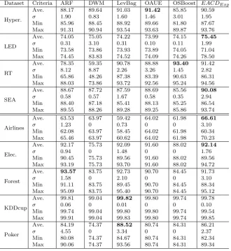
Table 6 Accuracy (%) of the methods compared in the immediate setting.
Dataset Criteria ARF DWM LevBag OAUE OSBoost EACDExp
Hyper.
Ave. 88.17 89.64 91.03 91.42 85.85 90.59 σ 1.90 0.83 1.60 1.46 3.01 1.95 Min 85.96 88.45 88.92 89.66 81.80 87.67 Max 91.31 90.94 93.54 93.63 89.87 93.76
LED
Ave. 74.05 75.05 74.22 73.99 74.15 75.45
σ 0.31 3.10 0.31 0.10 0.11 1.99 Min 73.58 73.86 73.93 73.89 74.05 71.04 Max 74.45 83.83 74.52 74.09 74.26 78.50
RT
Ave. 78.35 59.35 90.78 88.88 93.40 91.42 σ 8.12 8.87 2.26 3.26 1.45 2.82 Min 65.86 48.26 87.38 83.39 90.63 86.31 Max 88.03 73.86 93.72 92.56 95.24 94.56
SEA
Ave. 88.67 87.72 87.59 88.69 85.56 90.08
σ 0.58 0.57 1.67 0.58 0.35 2.94 Min 88.40 87.18 85.41 88.13 85.25 86.54 Max 89.55 88.26 89.28 89.25 85.86 93.74
Airlines
Ave. 63.53 63.97 59.42 64.02 61.98 66.61
σ 1.23 0 0.73 0 0 3.10
Min 62.08 63.97 58.45 64.02 61.98 60.34 Max 65.46 63.97 60.62 64.02 61.98 70.23
Elec.
Ave. 92.17 75.73 92.09 91.60 88.02 92.14
σ 0.94 0 1.48 0 0 1.76
Min 90.45 75.73 89.56 91.60 88.02 89.56 Max 93.19 75.73 93.70 91.60 88.02 94.72
Forest
Ave. 93.57 83.75 92.73 90.70 84.45 91.73
σ 1.58 0 2.10 0 0 3.10
Min 91.11 83.75 89.45 90.70 84.45 88.34 Max 95.09 83.75 95.40 90.70 84.45 95.12
KDDcup
Ave. 99.81 99.04 99.82 99.80 99.74 99.78
σ 0.06 0 0.01 0 0 0.10
Min 99.74 99.04 99.80 99.80 99.74 99.54 Max 99.91 99.04 99.83 99.80 99.74 99.85
Poker
Ave. 84.19 74.37 88.52 80.74 84.31 86.21
σ 4.55 0 3.34 0 0 2.37
Min 80.08 74.37 84.67 80.74 84.31 82.34 Max 90.06 74.37 93.56 80.74 84.31 89.34
the best average accuracy over four datasets, LevBag performs the best over two datasets, while OAUE, OSBoost and ARF achieve the best accuracy over one dataset. In the delayed setting (Table 7), EACDExp has the best aver-age accuracy over five datasets, OAUE achieves the best performance over two datasets, while OSBoost and LevBag achieve the best accuracy over one dataset.
Table 8 shows the overall evaluation CPU-time of the proposedEACDExp method compared to the other methods. For the majority of the datasets, DWM and OSBoost achieve the shortest evaluation time by far, whileEACDExp has the longest evaluation time for the majority of the datasets.
Table 7 Accuracy (%) of the methods compared in the delayed setting.
Dataset Criteria ARF DWM LevBag OAUE OSBoost EACDExp
Hyper.
Ave. 88.05 89.41 90.77 91.10 85.74 90.02 σ 2.02 0.95 1.71 1.59 3.06 2.01 Min 85.56 88.25 88.60 89.21 81.70 86.64 Max 91.35 90.86 93.37 93.55 89.78 92.95
LED
Ave. 74.00 74.14 74.21 74.06 74.13 75.26
σ 0.40 0.16 0.15 0.14 0.04 1.33 Min 73.62 73.99 74.07 73.93 74.10 72.94 Max 74.49 74.30 74.36 74.19 74.17 77.04
RT
Ave. 78.24 59.49 90.91 88.72 85.53 91.05
σ 8.06 8.67 2.48 5.13 2.90 3.75 Min 65.81 49.16 86.94 82.17 81.17 84.64 Max 87.92 73.73 93.69 93.47 88.70 94.56
SEA
Ave. 88.94 87.48 88.70 88.54 85.31 89.22
σ 0.59 1.02 1.45 0.70 0.42 2.43 Min 88.28 86.01 86.89 87.81 84.92 86.04 Max 89.51 88.21 90.32 89.21 85.91 91.89
Airlines
Ave. 61.42 60.57 58.49 62.73 61.80 63.35
σ 1.12 0 0.89 0 0 3.78
Min 61.22 60.57 57.03 62.73 61.80 59.06 Max 63.32 60.57 59.65 62.73 61.80 68.34
Elec.
Ave. 83.51 67.43 81.78 80.20% 79.04 85.03
σ 1.19 0 0.88 0 0 2.50
Min 81.78 67.43 80.54 80.20 79.04 80.45 Max 84.80 67.43 83.00 80.20 79.04 88.85
Forest
Ave. 85.65 74.93 86.22 86.84 74.47 84.83
σ 02.60 0 2.72 0 0 2.36
Min 83.67 74.93 84.30 86.84 74.47 81.45 Max 90.49 74.93 84.30 86.84 74.47 88.23
KDDcup
Ave. 99.80 99.12 99.81 99.78 99.74 99.76
σ 0.07 0 0.01 0 0 0.11
Min 99.72 99.12 99.79 99.78 99.74 99.48 Max 99.90 99.12 99.83 99.78 99.74 99.84
Poker
Ave. 67.95 59.31 76.78 73.81 81.23 80.21
σ 2.92 0 3.72 0 0 2.01
Min 64.94 59.31 70.51 73.81 81.23 76.35 Max 73.29 59.31 79.34 73.81 81.23 83.24
Table 8 Average evaluation time (in seconds) of executing the methods compared in the immediate setting.
Dataset ARF DWM LevBag OAUE OSBoost EACDExp
Hyperplane 208 130 144 107 93 349
LED 188 851 246 227 174 423
RT 394 195 207 148 1141 607
SEA 751 98 409 139 162 880
Airlines 495 66 531 366 74 657
Electricity 7.73 1.48 5.12 3.05 2.06 10.45
Forest 153 148 206 180 114 935
KDDcup99 56 581 130 204 138 536
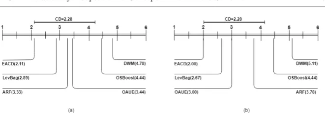
Table 9 Average rank of the methods compared.
Setting ARF DWM LevBag OAUE OSBoost EACDExp
Immediate 3.33 4.78 2.89 3.44 4.44 2.11
Delayed 3.78 5.11 2.67 3 4.44 2
different stages of the data stream (instance numbers 200K, 400K, 600K and 800K) in both the immediate (Figures 3(A, C, B and G)) and the delayed (Figures 3(B, D, F and H)) settings. In Figures 3(A) and 3(B), an abrupt concept drift centred in the instance number 200K is added with a width of 1. In Figures 3(C) and 3(D), a recurrent concept drift centred in the instance number 600K is added with a width of 1. In Figures 3(E) and 3(F), a gradual concept drift centred in the instance number 400K is added with a width of 10,000. And finally in Figures 3(G) and 3(H), a recurrent concept drift centred in the instance number 800K is added with a width of 10,000.
4.4 Statistical Analysis
The Friedman test [Friedman, 1940] is a non-parametric statistical test similar to the parametric repeated measures ANOVA (Analysis of Variance). It is used to detect differences across several algorithms in multiple test attempts (datasets). For this test, we need to demonstrate that the Null-hypothesis – stating that there is no significant difference between different algorithms – is rejected [Demˇsar, 2006].
The Friedman test is distributed according to Equation 5 withk−1 degrees of freedom:
χ2F = 12N k(k+ 1)
" k X
j=1
R2j−k(k+ 1) 2
4
#
, (5)
where Rj is the rank of the j-th of k algorithms and N is the number of datasets. Table 9 shows the average rank of each method included in the experiments in both the immediate and the delayed settings.
Note that for each setting,k= 6 andN = 9, as there are six methods and nine different datasets. Providing the value of the Friedman test statistic is χ2
F = 12.49 for the immediate setting andχ 2
F = 17.38 for the delayed setting with 5 (k−1) degrees of freedom, and the critical value for the Friedman test givenk= 6 andN = 9 is 10.78 at significance levelα= 0.05, we can conclude that the accuracy values of the studied methods are significantly different in both settings as theirχ2
F values (12.49 and 17.38) are greater than the critical value (10.78).
Fig. 3 Behaviour of the methods compared upon different concept drifts added to the SEA dataset in the immediate setting (left column; A,C,E and G) and the delayed setting (right column; B,D,F and H). The red boxes indicate the location and the length of the added concept drifts.
Fig. 4 Nemenyi test with 90% confidence level for (a) immediate and (b) delayed setting.
5 Discussion
As can be observed from Tables 3, 4 and 5, the average accuracy values of the explicit variations (EACDExp and EACDExp2) are slightly better than that of the implicit variations (EACDImp and EACDImp2). Furthermore, the accuracy values of the variations that use the GA optimisation technique are significantly better than that of the base variations for all datasets. By looking at the results of EACDbase, EACDbase4 and EACDExp, it can be concluded that using a concept drift detection mechanism alone cannot im-prove the results significantly, whereas using the concept drift detector along with a stochastic optimiser (GA) improves the accuracy significantly.
Among the variations that use only the base layer of the proposed algo-rithm, those that use a higher number oftypesand a higher number of features in eachtype (EACDbase4andEACDbase) are performing better compared to the other variations in the majority of the experiments. This is because the former variations create more classifiers on each time-step, with each classifier covering more features itself. This also justifies why they are more time con-suming compared to the other base-layer variations. Furthermore, when using a concept drift detection mechanism along with the base layer inEACDbase4 variation, it fails to improve the accuracy significantly compared to the vari-ation with the same parameters but without using a concept drift detector in EACDbase (improving only by 0.25% in the immediate and by 0.33% in the delayed setting). The explanation for this might be that while concept drift detectors can be very helpful for achieving a fast reaction to evolving data, they can also be destructive upon false alarms, especially when trained classifiers are removed immediately upon concept drifts.
de-pends greatly on the initial selection of the features. In the implicit and the explicit variations however, the combination of the features in each subspace is reconstructed by GA when needed.
The difference between the implicit and the explicit variations of the pro-posed method is the time it takes them to decide when to let GA start optimis-ing a set of subspaces usoptimis-ing the buffer of recently stored instances. Since the average accuracy ofEACDExp is about 1.13% higher than that ofEACDImp in the immediate setting and 1.02% higher in the delayed setting, we can con-clude that one of the most challenging parts of the proposed architecture is to decide when GA needs to reconstruct the combination of classification types in the genetic layer.
When looking at the values of the standard deviation for the real-world datasets used in the experiments (Tables 6 and 7), it can be noticed that DWM, OAUE and OSBoost have the same standard deviation of zero for all real-world datasets, whereas RD3+GA, LevBag and ARF have different stan-dard deviation values. This is because the latter algorithms use randomisation in their procedures, whereas the former do not. Since the experiments over the real-world datasets are repeated 10 times over the same data, the results obtained from all deterministic algorithms in all iterations are the same.
It can be further noticed from Tables 6 and 7 that for the artificial datasets, the standard deviation values for OSBoost, OAUE and DWM vary greatly throughout the experiments, reaching the value of about 8% for the RT dataset. At the same time, the standard deviation values for LevBag, ARF andEACDExp do not vary a lot, hardly reaching the value of 3.78%. This might be because the first three methods (OSBoost, OAUE and DWM) are implicit and do not use any concept drift detection mechanisms, whereas the other methods (Lev-Bag, ARF andEACDExp) are explicit and use concept drift detection mecha-nisms. As explicit methods have an immediate reaction to concept drifts, their accuracy does not drop for a long time throughout the experiments.
Form Table 8, it can be noticed that DWM has the lowest evaluation time over four datasets, OSBoost – over three datasets, whereas ARF and OAUE – over one dataset. The main drawback of the EACDExp variation of the proposed algorithm is its evaluation time, which is the longest for the majority of the datasets (six out of nine). The main reason for this is that this variation uses two different evolutionary algorithms (RD and GA) along with a concept drift detection method (EDDM). However, the other variations of the proposed algorithm offer slightly shorter evaluation times inEACDImp and EACDImp2, and significantly shorter times in EACDbase, EACDbase2 and EACDbase3. This is because the implicit variations of the EACD algorithm use both evolutionary algorithms but no concept drift detection method, while the base variations use only one evolutionary algorithm (RD) with no drift detection method.
more drastic in ARF compared to EACDExp. The reason for this might be their explicit strategy allowing to detect concept drifts as soon as they occur and use their recovery mechanism. In addition, detecting abrupt concept drifts should be easier for the concept drift detectors as the data distribution changes suddenly in such drifts. Furthermore, using different randomtypes in the base layer of EACDExp can result in a more robust performance, especially over drifting data, when the data distribution is not known in advance. DWM, OAUE and LevBag cope with concept drifts more slowly compared to ARF andEACDExp, while OSBoost seems to fail to adapt to the introduced abrupt concept drift in a good time.
In Figures 3(C) and 3(D), where a recurrent concept drift (with a width of one) occurred in the instance number 600K, the accuracy of all methods dropped, with EACDExp taking less time to adapt to the new data distri-bution and gain its average accuracy back again in both the immediate and the delayed settings. This might be because the proposed method uses two different mechanisms to cope with new environments: one (RD) weights the classificationtypesbased on their performance, while the other (GA) optimises the combination of the attributes of thesetypes.
In Figures 3(E) and 3(F), where a gradual concept drift (with a width of 10,000 and centred in the instance number 400K) occurred, it is clear that EACDExp copes with this concept drift in a more robust manner compared to the other methods in both settings. In the situations when a concept drift happens gradually, the time of detecting the drift plays an important role in how the drift is addressed, since the majority of the explicit methods start their adaptation procedure at that time. Hence, failing to detect the drift on time can cause the methods to suffer from the late adaptation. In the proposed method however, adaptation to the drifts can be divided into two stages: (1) before the drift is detected, when the algorithm tries to seamlessly adapt to the drift using RD; and (2) after the drift is detected, when GA starts to optimise the combination of the attributes in the genetic layer. This justifies the better performance of the proposed method, especially upon gradual concept drifts. In Figure 3(G), where a recurrent concept drift (with a width of 10,000) occurred in the immediate setting, the accuracy of all methods dropped within the same rate. However, EACDExp took less time to adapt compared to the other methods. In Figure 3(H), where the the same drift is shown in the delayed setting, the behaviour of all methods except OSBoost is relatively similar; how-ever, the accuracy ofEACDExp degrades less than that of the other methods during the drifting period (shown by the red box). In both settings, OSBoost fails to continue improving its performance for at least 14,000 instances from the instance number 805K. This behaviour of OSBoost is similar to its results upon abrupt and gradual concept drifts, which shows that the method lacks a sound adaptation mechanism over different types of concept drifts.
havethe fastest reaction over evolving dataon most occasions, especially upon abrupt, gradual and recurrent concept drifts, as shown in Figure 3.
While the proposed method is specifically designed to cope with non-stationary environments, it is possible to use it in non-stationary environments. However, the main limitation in this case would be the unnecessary overhead that the algorithm puts on the ensemble since the algorithm always builds classifiers over different time-stamps of the target data stream, while there is no need to do that, when a data stream does not evolve.
6 Conclusion and Future Work
In this paper, we proposed a novel method to seamlessly adapt to concept drifts in non-stationary data stream classification. The Evolutionary Adaptation to Concept Drifts (EACD) method has two layers with a set of classifiers in each layer. The first layer (base layer) is constructed by creating randomly drawn set of subspaces (classification types) from the pool of features of the target data stream. Eachtype is the basis for building decision trees (classifiers) in a layer. To seamlessly adapt to concept drifts in our approach, the Replicator Dynamics algorithm is used to increase or reduce the number of trees in each type according to their recent performance in the data stream. The second layer (genetic layer) uses randomly drawn subspaces from the first layer as the first population for Genetic Algorithm employed to optimise the classification types with the most recent instances. Creating new classifiers and training the current classifiers in this layer is the same as in the base layer. For the genetic layer, two different mechanisms are proposed to determine when to restart Genetic Algorithm. The first mechanism is based on comparing the performance of the two layers (implicit EACD), whereas the second one uses a concept drift detection method to check when a new concept drift occurs (explicit EACD).
To test the proposed method and its variations, a set of experiments with five real-world and four artificial datasets was conducted. First, the perfor-mance of different variations of the proposed method was compared; then, the best performing variation was compared to the state-of-the-art methods proposed in the literature. All experiments were conducted in two different settings: the immediate prequential and the delayed prequential. The results showed that our method achieves the highest average accuracy and the best average rank among all methods in both settings. However, the overall evalu-ation time of the proposed method is the longest in six out of nine datasets, which makes the evaluation time to be the main drawback of EACD.
The presented work opens the door to new developments that need to be theoretically analysed and practically tested in the future. The following ideas are proposed, to mention some.
– Detecting the classificationtypes that have not been useful for a long time in different environments to remove them and eventually make a room for new, better performingtypes to be added.
– Using dynamic instead of static weights for the base and the genetic layers of the method to have a potentially more robust weighting mechanism.
– Using a different removal mechanism when the maximum number of trees for a classification type is reached and a classifier (decision tree) should be removed; e.g. removing the oldest classifier inside the type instead of removing the worst performing one, as it is proposed in this paper.
– Adding the good performing classification types that are produced in the genetic layer to the base layer to keep them in the ensemble since the later layer can be cleared after some time. This can help optimising the algorithm, especially regarding the time criterion.
– Developing a pattern recognition system to track the usability of each type in different environments. This can lead to knowing thetypes better and using such information when data evolve, especially when a recurring concept drift occurs.
– Introducing a new concept drift detection system by analysing the be-haviour of the classification types.
References
[Baena-Garc´ıa et al., 2006] Baena-Garc´ıa, Manuel, Jos´e del Campo- ´Avila, Ra´ul Fidalgo, Albert Bifet, Ricard Gavald`a, & Rafael Morales-Bueno 2006. Early drift detection method. [Bifet & Gavalda, 2007] Bifet, Albert, & Ricard Gavalda 2007. Learning from time-changing data with adaptive windowing. In Proceedings of the 2007 SIAM International Conference on Data Mining, pages 443–448. SIAM.
[Bifet et al., 2010a] Bifet, Albert, Geoff Holmes, Richard Kirkby, & Bernhard Pfahringer 2010a. Moa: Massive online analysis. Journal of Machine Learning Research, 11(May):1601–1604.
[Bifet et al., 2010b] Bifet, Albert, Geoff Holmes, & Bernhard Pfahringer 2010b. Leverag-ing baggLeverag-ing for evolvLeverag-ing data streams. Machine LearnLeverag-ing and Knowledge Discovery in Databases, pages 135–150.
[Bifet et al., 2009] Bifet, Albert, Geoff Holmes, Bernhard Pfahringer, Richard Kirkby, & Ricard Gavald`a 2009. New ensemble methods for evolving data streams. In Proceedings of the 15th ACM SIGKDD international conference on Knowledge discovery and data mining, pages 139–148. ACM.
[Blackard & Dean, 1999] Blackard, Jock A, & Denis J Dean 1999. Comparative accuracies of artificial neural networks and discriminant analysis in predicting forest cover types from cartographic variables. Computers and electronics in agriculture, 24(3):131–151. [Bomze, 1983] Bomze, Immanuel M 1983. Lotka-Volterra equation and replicator dynamics:
a two-dimensional classification. Biological cybernetics, 48(3):201–211.
[Breiman, 2001] Breiman, Leo 2001. Random forests. Machine learning, 45(1):5–32. [Breiman et al., 1984] Breiman, Leo, Jerome Friedman, Charles J Stone, & Richard A
Ol-shen 1984. Classification and regression trees. CRC press.
[Brzezinski & Stefanowski, 2014b] Brzezinski, Dariusz, & Jerzy Stefanowski 2014b. React-ing to different types of concept drift: The accuracy updated ensemble algorithm. IEEE Transactions on Neural Networks and Learning Systems, 25(1):81–94.
[Chen et al., 2012] Chen, Shang-Tse, Hsuan-Tien Lin, & Chi-Jen Lu 2012. An online boost-ing algorithm with theoretical justifications. arXiv preprint arXiv:1206.6422.
[Chu & Zaniolo, 2004a] Chu, Fang, & Carlo Zaniolo 2004a. Fast and light boosting for adaptive mining of data streams. In Pacific-Asia Conference on Knowledge Discovery and Data Mining, pages 282–292. Springer.
[Chu & Zaniolo, 2004b] Chu, Fang, & Carlo Zaniolo 2004b. Fast and light boosting for adaptive mining of data streams. In Pacific-Asia Conference on Knowledge Discovery and Data Mining, pages 282–292. Springer.
[Cup, 1999] Cup, KDD 1999. Data (1999). URL: http://kdd. ics. uci. edu/databases/kddcup99/kddcup99. html.
[Demˇsar, 2006] Demˇsar, Janez 2006. Statistical comparisons of classifiers over multiple data sets. Journal of Machine learning research, 7(Jan):1–30.
[Domingos & Hulten, 2000a] Domingos, Pedro, & Geoff Hulten 2000a. Mining high-speed data streams. In Proceedings of the sixth ACM SIGKDD international conference on Knowledge discovery and data mining, pages 71–80. ACM.
[Domingos & Hulten, 2000b] Domingos, Pedro, & Geoff Hulten 2000b. Mining high-speed data streams. In Proceedings of the sixth ACM SIGKDD international conference on Knowledge discovery and data mining, pages 71–80. ACM.
[Elwell & Polikar, 2011] Elwell, Ryan, & Robi Polikar 2011. Incremental learning of concept drift in nonstationary environments. IEEE Transactions on Neural Networks, 22(10):1517– 1531.
[Elyan & Gaber, 2017] Elyan, Eyad, & Mohamed Medhat Gaber 2017. A genetic algorithm approach to optimising random forests applied to class engineered data. Information sciences, 384:220–234.
[Fawgreh et al., 2015] Fawgreh, Khaled, Mohamed Medhat Gaber, & Eyad Elyan 2015. A replicator dynamics approach to collective feature engineering in random forests. In Re-search and Development in Intelligent Systems XXXII, pages 25–41. Springer.
[Folino et al., 2006] Folino, Gianluigi, Clara Pizzuti, & Giandomenico Spezzano 2006. GP ensembles for large-scale data classification. IEEE Transactions on Evolutionary Compu-tation, 10(5):604–616.
[Folino et al., 2007] Folino, Gianluigi, Clara Pizzuti, & Giandomenico Spezzano 2007. An adaptive distributed ensemble approach to mine concept-drifting data streams. In Tools with Artificial Intelligence, 2007. ICTAI 2007. 19th IEEE International Conference on, volume 2, pages 183–188. IEEE.
[Friedman, 1940] Friedman, Milton 1940. A comparison of alternative tests of significance for the problem of m rankings. The Annals of Mathematical Statistics, 11(1):86–92. [Gama et al., 2014] Gama, Jo˜ao, Indr ˙e ˇZliobait ˙e, Albert Bifet, Mykola Pechenizkiy, &
Ab-delhamid Bouchachia 2014. A survey on concept drift adaptation. ACM Computing Surveys (CSUR), 46(4):44.
[Gen & Cheng, 2000] Gen, Mitsuo, & Runwei Cheng 2000. Genetic algorithms and engi-neering optimization, volume 7. John Wiley & Sons.
[Gomes et al., 2017a] Gomes, Heitor Murilo, Jean Paul Barddal, Fabr´ıcio Enembreck, & Albert Bifet 2017a. A Survey on Ensemble Learning for Data Stream Classification. ACM Computing Surveys (CSUR), 50(2):23.
[Gomes et al., 2017b] Gomes, Heitor M, Albert Bifet, Jesse Read, Jean Paul Barddal, Fabr´ıcio Enembreck, Bernhard Pfharinger, Geoff Holmes, & Talel Abdessalem 2017b. Adaptive random forests for evolving data stream classification. Machine Learning, pages 1–27.
[Gomes & Enembreck, 2013] Gomes, Heitor Murilo, & Fabr´ıcio Enembreck 2013. Sae: Social adaptive ensemble classifier for data streams. In Computational Intelligence and Data Mining (CIDM), 2013 IEEE Symposium on, pages 199–206. IEEE.